
A Comparison of Numerical Schemes for Simulating Reflected Wave on Dry and Enclosed Domains

1
Faculty of Water Resources Engineering, Thuyloi University, Ha Noi 116705, Vietnam
2
Hydraulic Construction Institute, Ha Noi 116705, Vietnam
*
Author to whom correspondence should be addressed.
Water 2023, 15(15), 2781; https://doi.org/10.3390/w15152781
Submission received: 11 June 2023
/
Revised: 25 July 2023
/
Accepted: 27 July 2023
/
Published: 31 July 2023
(This article belongs to the Section Hydraulics and Hydrodynamics)
Abstract
:This paper is to investigate the capability of six numerical schemes to simulate reflected wave over a dry and closed domain with and without building, namely: (a) two proposed 2D numerical models solving the conservation form of 2D Shallow Water Equations (2D-SWEs) by Finite Volume Method (FVM) with Roe and HLLC schemes are invoked to approximate Reimann solver; (b) three options of shallow models in the commercial software Flow 3D based on a non-conservation form of 2D-SWEs and (c) the Flow 3D with turbulence modules. By analyzing flooding maps, the area of the reflected wave, and water level profiles on a dry and closed domain, two proposed models give reasonable solutions, while three options of the shallow module of Flow 3D originate result less accurately when initial wave celerity (c0) is small. The accuracy level will be increased if c0 value increases. The 3D model presented the best performance of the complex flow pattern in the dry and enclosed domain in both cases without and with building.
1. Introduction
Flood waves are often considered a complex physical process that presents a difficult modeling challenge. Further, the presence of any man-made structure downstream may function as a vertical wall or building. A reflected wave occurs and propagates with a high speed towards the dam axis, then interacts with each other. As a result, a complicated flow pattern may occur in the enclosed domain. Several studies have examined the propagation of flood waves and the interaction between rapid flows and structures [1,2,3,4].
The 2D depth-averaged shallow water model is generally accepted to predict the main flow features for flood hazard assessment and flood risk management [5,6]. SWEs are valid when the vertical length scale is negligible compared to the horizontal one. In recent years, numerous research studies have used the finite volume Godunov-type method for the numerical solution of SWEs [6,7]. The numerical intercell fluxes were often evaluated by Roe or HLLC scheme. A large amount of literatures applied Roe method [8,9] and HLLC one [10,11]. In addition, they provided valuable results while using considerably less computational time [6,7,9]. Further, a number of efficient user-oriented software programs are currently available to facilitate the use of depth-averaged numerical models for free-surface flow simulations, such as HEC-RAS 2D or Telemac 2D (e.g., [12,13,14]), or module shallow water of Flow 3D [4,15]. These literatures pointed out that 2D SWE models can model well flow depths and discharge partition in floods, but not always accurately reproduce velocity patterns [16]. On the other hand, there has been a limited amount of research devoted to evaluating numerical schemes for the forward and backward wavefront caused by dry and enclosed domain [15]. In this case, the effect of resistance of dry bed and the complex hydraulic jump yielded by the interaction of forward and backward waves during computation tends to introduce numerical instabilities in the solution [6,9]. Kocaman (2021) pointed out that the flow pattern of dam break wave in the enclosed domain without building were quite complex due to the effect of vertical walls at boundaries [15]. However, this study did not investigate the influence of building on dam break wave. On the other hand, the common experiment hydraulic aspects used to calibrate and validate numerical models were: time series of flow depth, velocity, pressure as well as the image recordings [17]. However, assessment of flooding map based on only the wetted area did not show clearly the influence of structures or given numerical schemes on numerical results. Therefore, the authors proposed a new technique by separating forward wave and backward wave area to evaluate in detail this influence.
Due to its robustness, effectiveness, and accuracy, the 3D Computational Fluid Dynamics (CFD) models have been widely used in a wide range of hydrodynamic issues recently [18,19,20,21]. Flow 3D is one of the well-known CFDs, so there are numerous applications of this model in several hydraulic problems [22,23,24]. Solving the Reynolds-Averaged Navier-Stokes (RANS) equations combined with a turbulence model can provide an accurate description of dam-breaking waves [15,25]. Nevertheless, the shallow module of Flow 3D based on 2D SWEs is rarely applied in large computational domains despite the fact that computational time is cheaper than that of 3D models. The investigation of Kocaman (2021) showed that inundated maps and flow depth profiles obtained by the shallow module of Flow 3D were reasonable [15]. However, in this literature, initial water level in reservoir h0 = 0.15 m was large, which may yield the free surface flow dismissing 3D hydraulic characteristics at downstream. This point should be verified with smaller value of h0 to fulfill this discover, because the smaller h0 was, the shallower flow depth at downstream got. In such case, the effect of vertical acceleration in the shallow depth flow was greater than that in the deeper flow.
Therefore, this research examines the capability of five 2D numerical models and a 3D model to simulate forward and backward wavefront trajectories due to the dry and enclosed domain with and without building. Five 2D CFD models are involved: two numerical models based on finite volume Godunov-type method to solve 2D SWEs and intercell fluxes are approximated by Roe and HLLC schemes; three options of shallow module of Flow 3D model controlled the order of accuracy of advection in the fluid momentum equations, which including the first-order accuracy, the second-order accuracy and the second order monotonicity-preserving. The 3D model was taken from Flow-3D commercial software, solving the 3D Reynolds-Averaged Navier-Stokes (RANS) with the RNG k-ω turbulence model for closure. Three achievements of this study can be listed: (a) to compare the capability of six numerical schemes in performance flow regime in the dry and enclosed domain by series of snapshots flooding map, area of the reflected wave and the stage hydrographs; (b) to propose a new technique in quantifying flooding map; and (c) to point out that the accuracy level of predicted results obtained by a shallow module of Flow 3D increases when initial wave velocity increases.
2. Materials and Methods
2.1. 2D Shallow Water Equations
By neglecting vertical acceleration and assuming a hydrostatic pressure distribution, the two-dimensional shallow water equations are derived by considering the depth-Averaged Navier-Stokes equations in three dimensions. The conservation forms of 2D-NSWE can be represented by Equation (1):
where:
with
with
V indicates the vector of conserved variables; K and H are flux vectors, and S is a source term accounting for the bed slope term S1 and friction term S2; x, y are orthogonal space coordinates on a horizontal plane; t is time; h and zb represent flow depth and bottom elevation; u, v are velocity components in the x and y directions; S0x, S0y are bed slope terms in x and y axes. In the case of a horizontal bed, bed slope term S1 can be ignored. Sfx, Sfy are bed slopes and friction slopes along the same directions; n is the Manning roughness coefficient; g is gravity acceleration.
Based on the finite volume Godunov-type method to solve 2D SWEs, the flow variables are updated to a new time step by using Equation (2):
where n denotes time level, i and j are space indexes of cell along x and y directions; Δt, Δx, Δy are time step and space sizes of the computational cell.
Additionally, interface fluxes and are approximated by both HLLC and ROE approximate Riemann solver [8,10]. Friction terms was treated by semi implicited method and to avoid unphysical flow inversion while bed slope terms was solved by the technique of local reconstruction of bed elevation to satisfy mass conservation [9].
A numerical code, namely 2D-FVM, based on both HLLC and ROE schemes, was written in the Fortran language by the first author. This program has been successfully applied for dam-break wave simulation in previous research [25,26]. However, the 2D-FVM model still has some limitations, such as: (i) the numerical scheme is explicit, so time-consuming, and expensive; (ii) using structure mesh in all computational domains cannot capture well hydraulic characteristics at the complex domain or abrupt topography. Mesh refinement is necessarily required at this location to have a better solution.
2.2. Flow 3D Model
2.2.1. 3D Navier-Stokes Equations
The FVM in Flow-3D software allows simultaneous solution of three-dimensional motion RANs and continuity equations. Continuity and motion equations in Cartesian coordinates are given below:
where p is pressure, ρ is fluid density, ui accounts for the flow velocity in direction i, Aj is a fractional area of the fluid in each cell, Vf is the volume fraction of the fluid in each cell, Gi, fi are the body acceleration and viscous acceleration in the direction i.
In fact, turbulence phenomena have always appeared in most physical processes. It would be able to perform simulations with the equations of mass and momentum conservation based on Navier-Stokes if the mesh resolution is sufficient to capture such details. However, this is generally not possible because of the limitations of computer memory and processing time. Therefore, computational fluid dynamics (CFD) methods must be simplified by using modeling that describes the effects of turbulence on the mean flow characteristics. Within six turbulence models in Flow 3D: the Prandtl mixing length, the family of RANs, Renormalization Group (RNG), k-ω model and the Large Eddy Simulation model (LES), which requires more effort due to the finer-than-usual meshes, the RNG model is known to describe low intensity turbulence flows and flows having strong shear regions more accurately [25,27]. Therefore, the authors selected this module to simulate propagation wave in dry and enclosed domain.
2.2.2. Shallow Models in Flow 3D
The SWE model of Flow-3D is used to solve complex flow dynamics in a wide range of engineering applications. This includes the simulation of liquid-gas flows, wave-structure interactions, and free-surface flows [28]. In the SWE model, the z-direction is assumed to be a shallow direction. Two real cells are considered in each mesh block in this direction. When depth-averaged velocity is applied to the momentum equation in the z-direction, it reduces to the hydrostatic Equation (4):
where p0 is atmospheric pressure on the free surface of the water, and H represents the height of the free surface above the bottom of the grid, which is the sum of the obstacle and water heights:
where δz is the cell size in z direction. Substitute H into Equation (4), we have: and apply depth-averaging to the three-dimensional momentum equations in the vertical direction; we obtain the momentum equations for the shallow water model.
Flow-3D allows solving non-conservative form of the 2D SWEs, which can be given as:
where t represents time, u and v are velocity components along x and y directions, gx and gy are body accelerations in x and y directions, respectively;
where CD represent the drag coefficient. This parameter should be taken to the value of 0.025 when downstream is dry [15]. The volume fraction (VF) and fluid fraction (F) are used for defining a variable bottom contour and fluid depth, respectively.
A generic form for the finite difference approximation of two momentum equations can be written [28]:
where FUX and FVX are the advective fluxes of u and v in the x direction; FUY and FVY are the advective flux of u and v in the y direction; Gx and Gy are gravitational terms in x and y directions; VISX and VISY are viscous term acceleration terms in x and y directions.
The advective flux FUX:
where
The basic idea of Equation (7) is to weight the upstream quantity being fluxed more than the downstream value. The weighting factors are (1 + α) and (1 − α) for upstream and downstream directions, respectively. If α = 0, this approximation reduces to a spatially second-order accurate, centered difference approximation. If α = 1.0, the first-order donor cell approximation is recovered. To employ a second-order accurate approximation for the advective and viscous accelerations in both time and space, two steps are produced: step 1: the first-order method is used with the donor cell parameter α = 1.0, then repeat with α = −1.0; step 2: the results of two calculations are averaged to give a desired second-order approximation to the new time level velocities.
The second-order, monotonicity-preserving upwind difference method employed in the Flow 3D model is based on the theory first introduced by [29]. For example, a variable Q advected in the x direction, the value fluxed through a cell face, Q∗ is computed as:
where:
- -
- Qi: the cell-centered value
- -
- C: the Courant number
- -
- A: second-order approximation to the first derivative of Q at the location within the cell.
The term Qi in Equation (8) gives the usual first-order donor cell approximation, while the second-order approximation is generated by the addition of the second term on the right side of this equation. To ensure monotonicity, it is necessary to restrict the value of the derivative A:
Furthermore, if Qi is a local minimum or maximum value, the two centered derivatives appearing in equation are opposite signs, then A is set to zero, and the donor cell approximation is used.
Therefore, some advantages and disadvantages of the three options controlled the order of accuracy of advection in the fluid momentum equations can be sorted [28]:
- First-order accuracy: The simplest and fastest method; most suitable for general flows;
- Second-order accuracy: This method is second-order accurate in both space and time. So, it is the most efficient method for minimizing numerical dissipation in swirling flows. However, this scheme does not process the transportive property. Further, this method may occasionally generate a numerically unstable solution for flows with transient-free surfaces;
- Second-order monotonicity-preserving: This method is second-order accurate in space and first-order accurate in time. It is useful when studying swirling, free-surface flows. A slight increase in CPU time is required over the first-order method, but in most cases, the difference is not significant.
2.3. Computational Domain
In order to examine the capability of 6 selected numerical models in simulating hydraulic jumps in dry and enclosed domains with and without building, two experiment tests taken from the study of Aureli (2011) were conducted [30]. After that, there was only Vacondio (2013) reproduced these tests to validate the smoothed particle hydrodynamics (SPH) method in solving 2D SWEs [31].
A rectangular tank divided into two compartments measured 2.6 m long and 1.2 m wide. The initial water level in the reservoir was 0.063 m, while the floodable area was dry (Figure 1).
2.4. Sensitivity Analysis
The accuracy of the numerical models was evaluated using statistical indicators. The Normalized Root Mean Square Error (NRMSE) and the Relative Error (E%) were given by Equations (10) and (11):
where Xi,exp and Xi,sim represented the experimental and numerical values of the X variable; Xexp,max and Xexp,min are maximum and minimum values of experiment data of X variable, respectively; N is the amount of data.
2.5. Mesh Convergence Analysis
The Grid Convergence Index (GCI) has been widely applied in many CFD studies to estimate the discretization error in the numerical solution [32,33]. The GCI indicated the degree of resolution and how much the simulation results approached the asymptotic value. So, a small GCI value meant the solution was in the asymptotic range. Three different structured meshes of 0.005 m, 0.006 m, and 0.0072 m corresponding with fine, medium, and coarse meshes were employed. Similarly to [34], in this study, the maximum water depths at three locations (G1, G2, and G3) simulated by the 3D model were used to compute the GCI value (Table 1).
As can be seen from Table 1, GCI reduces from coarse mesh to fine one (GCI32 > GCI21) at all gauges. Particularly, at gauge G1, the value of GCI reduces from 0.513% to 0.08% for GCI32 and GCI21, respectively, and at G2, this value gets 0.55% and 0.164%. It can be said that the grid-independent solution is nearly achieved and does not need to carry out further mesh refinement. Moreover, the value of GCI32/rpGCI21 close to 1 indicates that the numerical solutions are within the asymptotic range of convergence. As a result, the fine grid spacing of 0.005 m is sufficient to obtain a reliable numerical solution in the present study.
Six numerical schemes used in simulating two test cases, (A) without building and (B) with building, can be shown in Table 2. All simulations in this study were implemented on the Intel ® core™ i7-7820HQ CPU @ 2.9 GHz, RAM 16.0 Gb. Output time steps are taken to 0.05 s for all output data of the Flow 3D model. Computing time and file size are also shown in Table 2. Obviously, a 3D model requires much more computational time and effort to simulate dam break flow than 2D models based on SWEs. Both computational time and file size needed for the former are almost ten times for the latter. Therefore, 2D SW models are preferred over RANs-based model for problems requiring large computational domain of real case study.
3. Results and Discussion
3.1. Dam Break Wave in Dry and Enclosed Domain without Building
The first step of our investigation is to determine the possibility of three numerical schemes 1, 2, and 3 in the shallow water module of Flow 3D. The strong turbulence is observed in all numerical inundated maps (Figure 2). Compared with measured data, all numerical schemes predict the propagation of shock waves at an early stage (t = 1.4 s) with the same shape and area of the wetted area. At later times, three reflected waves produced undulating and overlapping in a complex way. The interaction between the forward and backward wavefront led to an oblique hydraulic jump. Despite this, the wavefront reflected against the channel sidewalls occupies a much larger area than the observed wavefront. Further, Figure 3 shows three reflected zones, SI, SII, and SIII, caused by three vertical boundaries. The percentage errors of reflected area (E%) presented in Table 3 indicated that a small value of E at t = 1.4 s (0.05% for model 1, 1.21% for model 2, and 0.28% for model 3) shows the close matching between numerical and experimental results. However, the dispersion and diffusion are witnessed at t = 3.4 s and 4.65 s. For example, the relative error (E%) at zone 3 is 95.43%, 58.55%, and 47.49% in accordance with models 1, 2, and 3, respectively (Table 3).
On the other hand, Figure 4 shows water level profiles at five gauges obtained by these models. The first-order accuracy scheme produces numerical results more stable than those obtained by models 2 and 3. Further, the NRMSE value shows that results at G1 and G2 near the dam site obtained by this model are better than solutions obtained by both second-order schemes. Results at G3, G4, and G5 near the downstream boundary witness the approximate value of NRMSE indexes. The numerical solutions generated by models 1, 2, and 3 at G2 show a large surge at the end, while others do not (Table 4). Although the RANs model has a high relative error of 9.32% at the early stages of dam failure, this value diminishes quickly at t = 3.4 s and 4.65 s when the relative error gets 0.94% and 0.6%, which are small in comparison to other models.
Besides flow depth hydrographs, velocity components in the x and y directions are also important hydraulic features in studying free surface flow. However, there is no empirical data on velocity components in Aureli’s work; a 3D numerical solution is considered as reference data to evaluate 2D results in Figure 5 because 3D numerical results of u and v showed very good agreement with experiment ones [25]. In general, the time series of u and v obtained by the 3D model are quite stable. All numerical data at gauge G2 closed with the dam gate are matching together. However, the numerical simulations at gauge G5 is strongly dispersion. The maximum values of u and v at gauge G5 obtained by models 1, 2, and 3 are quite larger than that obtained by model 4. Thus, it is necessary to have measured data of velocity to validate every numerical scheme.
Furthermore, Figure 6 and Figure 7 present inundated maps and water depth profiles that use the 3D RANs model and 2D models of ROE and HLLC. Obviously, the strong undulation almost disappears in all flood maps (Figure 6). The wavefronts reflected by the three side walls are quite similar to those observed empirically (at t = 3.4 s and 4.65 s). At t = 4.65 s, 3D results perform better than 2D ones because the backward wave does not reach the dam site, while 2D solutions barely touch the dam. Further, G1 and G2 indicate the trend of the flow depth profile obtained by turbulence module RANs is quite close to the observed one, while 2D solutions are underestimated (Figure 7). The arrival time of the forward wave interacting with the backward one formed by models 4, 5, and 6 can be captured well at all gauge points, while three modules of Flow 3D’s shallow cannot be predicted correctly (Figure 4 and Figure 7). The value of the statistical error indicator also proved that the NRMSE of 3D results is small except for point G4 (Table 4). This means the 3D numerical scheme is the best performance in case of rapid flow on dry and closed domains without obstacles.
In general, the flood extent of Flow 3D is reasonably represented by three options of the shallow 2D model. For inundated maps and flow depth profiles, first-order accuracy provides the best solution. The RANs model is the most accurate among the six selected numerical schemes. Two 2D numerical schemes by Roe and HLLC perform quite similarly in all hydraulic aspects. In the early stages of dam collapse, the overestimation of shock performance is still witnessed on flooding maps.
3.2. Dam Break Wave in Dry and Enclose Domain with Presence of Building
In addition, the presence of a building can make the flow regime more complicated due to the interaction of the dam break wave with the building. Figure 8 and Figure 9 demonstrate how intense undulation produces hydraulic jumps in a complex manner. However, the numerical instability is observed in numerical results obtained by three numerical schemes of the shallow module, while the formation of dam break wave generated by models 4, 5, and 6 are quite matching with the measured ones (Figure 8 and Figure 9). Numerical schemes 5 and 6 generate flood map formation quite similarly. At t = 4.0 s, the reflected wave on the left side performed by models 5 and 6 touches the dam site, while the solution of 3D does not (Figure 9). This means that the 3D solution is better than others. Further, it is found that three models, 1, 2, and 3, cause much more expansion of three reflected zones than the observations (Table 4). At t = 4.0 s, the percentage error of refected (SIII) are 39.59%, 69.20%, and 48.05% for three models 1, 2, and 3, respectively. However, the results obtained by models 4, 5, and 6 show more acceptable errors, although this value is greater than that in the case of the absence of the building (see Table 5). Further, the stage hydrographs presented in Figure 10 and Figure 11 show the oscillation occurring at almost all gauges (except G1). This hydraulic aspect yielded by models 1, 2, and 3 shows a downward trend at the last time, whereas the time series of observed data increase quickly and peak at this moment. This conclusion is also revealed by Table 6 when the NRMSE obtained by models 1, 2, and 3 at gauges G2, G3, and G4 are much greater than those yielded by models 4, 5, and 6.
Therefore, the presence of buildings within a dry and enclosed domain creates a complicated shockwave effect. Particularly, the significant disagreement of numerical flood extents is observed in three models: 1, 2, and 3. The intense fluctuation is formed in both flooding maps and stage hydrographs. NRMSE is so large at gauges G2, G3, and G4, with almost NRMSE values are greater than 0.3, that the accurate level cannot be accepted to some extent. This limitation may come from Flow 3D solving the non-conservative form of 2D−SWE. In contrast, two proposed numerical models used FVM to solve the conservation form of 2D SWEs give much better solutions when the undulation is reduced in all inundated maps. Water stage profiles and statistical error indicators (NRMSE) show reasonable trends and values, respectively, but their accuracy is less than 3D solution. This point shows that the coupling turbulence module in RAN equations can accurately simulate the non−hydrostatic, transmissive flow. Especially, at an early stage of dam collapse, or the presence of obstruction, it makes a significant impact on 3D hydraulic characteristics. This comment can be proved by the restimulation of the test case in the Kocaman study [15], which is presented in Section 3.3.
3.3. The Influence of Initial Wave Celerity on Dam Break Wave on Dry and Enclosed Domain
In a test case of dam break flow over dry and closed domain taken from [15], the initial water level (h0) was 0.15 m, corresponding with wave celerity = 1.213 m/s, which was greater than that in the previous test with c0 = 0.792 m/s (Figure 12). For evaluating the influence of c0 value on the numerical performance of dam break wave, three values of h0 0.05 m, 0.1 m, and 0.15 m corresponding with three values of c0 (m/s) 0.70, 0.99, and 1.21, respectively, were imposed to four models 1, 2, 3, 4 to reproduce the water level profiles at five gauges.
Figure 13 indicates the water stage profiles at five study points are quite close to the experimental data. Although, the fluctuations formed on 2D numerical results would be greater than those on 3D results. At the moment of reflected wave against forward one, the oscillation occurs strongly and then gradually decreases. 3D numerical data witness the best performance in comparison with empirical results, so it is taken as reference data for evaluating the influence of initial wave celerity c0 on 2D numerical results.
Gauge P1 in reservoir witneeses the greatest accuracy level when all NRMSE value is smaller than 0.02 (Table 7). With the smallest value of initial wave celerity, model 2 shows the best solutions at points P2 and P3 when the value of NRMSE is 0.0869. However, at the largest value, c0, model 3 performs better at these gauges but is less accurate than model 1 at points P4 and P5.
In general, the smaller the value of c0, the greater the NRMSE value gets, excluding some values obtained by model 1 (Table 7). This point illustrates that the accuracy of 2D numerical results increases when the initial wave celerity value increases. The reason can be explained that when flood depth is higher, the vertical acceleration component becomes negligible, leading to 2D simulation becoming more successful.
4. Conclusions
The objective of this study is to implement six numerical schemes to simulate dam break flow in a dry and closed domain with and without buildings.
In general, the presence of a building causes the formation of a hydraulic jump in a closed domain, which is more complicated than that of the case without a building. Regarding computing time and file size, the 2D SW models require much less time and computational resources than the 3D ones.
A program based on FVM solved the Reimann problem by Roe and HLLC schemes, producing flooding maps and water-stage profiles. The undulation oscillation phenomena have almost disappeared. That means the forward and backward wavefront can be captured well by these models. Nevertheless, the time series of flow depth is underestimated, and the moment these waves interact with each other is not captured accurately. In further study, the proposed program can be applied to real case studies.
Considering three numerical schemes of shallow modules in Flow 3D, all of them give 2D numerical results of water stage and flooding maps less exactly than those obtained by two proposed 2D numerical models and 3D ones. When the initial wave of celerity is small, the first-order scheme produces a solution more stable than the two second-order ones. This limitation is due to the use of the non-conservation form of 2D SWEs in the shallow model of Flow 3D. Additionally, shallow flood flows may have fully 3D hydraulic characteristics, while SW models cannot simulate non-hydrostatic flows correctly. In contrast, if the c0 value increases, the vertical velocity component becomes insignificant. As a result, all SW model options perform dam break waves more successfully.
Moreover, the RANs model with RNG turbulence closure has the most accurate capability in simulating the complex hydraulic jump on dry and enclosed domains with and without building. Particularly, at the early stage of a dam break and at the front of the dam breaking wave will walls or buildings, the 3D model can perform well the 3D flow characteristics with many complicated hydraulic phenomena while 2D models are not able to simulate.
However, structure mesh is used in both 2D and 3D models, so mesh refinement should be required at the complex domain or abrupt topography to obtain an accurate numerical solution.
Besides using NRMSE and E (%) criteria in evaluating numerical results of stage hydrograph, the evaluation area of the reflected wave instead of assessing only the wetted area and shape of the flooding map can contribute to assessing flood hazard more accurately.
Author Contributions
Conceptualization, L.T.T.H.; Methodology and writing, L.T.T.H.; Formal analysis, L.T.T.H. and N.V.C.; Simulation, L.T.T.H. and N.V.C. All authors have read and agreed to the published version of the manuscript.
Funding
This research received no external funding.
Institutional Review Board Statement
Not applicable.
Informed Consent Statement
Not applicable.
Data Availability Statement
Data sharing is not applicable.
Conflicts of Interest
The authors declare no conflict of interest.
References
- Mignot, E.; Li, X.; Dewals, B. Experimental modelling of urban flooding: A review. J. Hydrol. 2019, 568, 334–342. [Google Scholar] [CrossRef] [Green Version]
- Soares-Frazão, S.; Zech, Y. Dam-break flow through an idealised city. J. Hydraul. Res. 2008, 46, 648–658. [Google Scholar] [CrossRef] [Green Version]
- Shige-eda, M.; Akiyama, J. Numerical and Experimental Study on Two-Dimensional Flood Flows with and without Structures. J. Hydraul. Eng. 2003, 129, 817–821. [Google Scholar] [CrossRef]
- Kocaman, S.; Ozmen-Cagatay, H. Investigation of dam-break induced shock waves impact on a vertical wall. J. Hydrol. 2015, 525, 1–12. [Google Scholar] [CrossRef]
- Ye, Y.; Xu, T.; Zhu, D.Z. Numerical analysis of dam-break waves propagating over dry and wet beds by the mesh-free method. Ocean Eng. 2020, 217, 107969. [Google Scholar] [CrossRef]
- Aureli, F.; Maranzoni, A.; Mignosa, P.; Ziveri, C. A weighted surface-depth gradient method for the numerical integration of the 2D shallow water equations with topography. Adv. Water Resour. 2008, 31, 962–974. [Google Scholar] [CrossRef]
- Maranzoni, A.; Tomirotti, M. New formulation of the two-dimensional steep-slope shallow water equations. Part I: Theory and analysis. Adv. Water Resour. 2022, 166, 104255. [Google Scholar] [CrossRef]
- Roe, P. A basis for upwind differencing of the two-dimensional unsteady Euler equations. In Numerical Methods in Fluids Dynamics II; Oxford University Press: Oxford, UK, 1986. [Google Scholar]
- Brufau, P.; García-Navarro, P.; Vázquez-Cendón, M.E. Zero mass error using unsteady wetting-drying conditions in shallow flows over dry irregular topography. Int. J. Numer. Methods Fluids 2004, 45, 1047–1082. [Google Scholar] [CrossRef]
- Toro, E.F. Shock-Capturing Methods for Free-Surface Shallow Flows; John Wiley & Sons: Hoboken, NJ, USA, 2001. [Google Scholar]
- Liang, Q. Flood Simulation Using a Well-Balanced Shallow Flow Model. J. Hydraul. Eng. 2010, 136, 669–675. [Google Scholar] [CrossRef]
- Sharma, V.C.; Regonda, S.K. Two-dimensional flood inundation modeling in the godavari river basin, India—Insights on model output uncertainty. Water 2021, 13, 191. [Google Scholar] [CrossRef]
- Pilotti, M.; Milanesi, L.; Bacchi, V.; Tomirotti, M.; Maranzoni, A. Dam-Break Wave Propagation in Alpine Valley with HEC-RAS 2D: Experimental Cancano Test Case. J. Hydraul. Eng. 2020, 146, 05020003. [Google Scholar] [CrossRef]
- Robins, P.E.; Davies, A.G. Application of T ELEMAC -2D and SISYPHE to complex estuarine regions to inform future management decisions. XVIIIth Telemac Mascaret User Club 2016, 2011, 86. [Google Scholar] [CrossRef]
- Kocaman, S.; Evangelista, S.; Guzel, H.; Dal, K.; Yilmaz, A.; Viccione, G. Experimental and numerical investigation of 3d dam-break wave propagation in an enclosed domain with dry and wet bottom. Appl. Sci. 2021, 11, 5638. [Google Scholar] [CrossRef]
- Dewals, B.; Kitsikoudis, V.; Mejía-morales, M.A.; Archambeau, P.; Mignot, E. Can the 2D shallow water equations model flow intrusion into buildings during urban floods? J. Hydrol. 2023, 619, 129231. [Google Scholar] [CrossRef]
- Medeiros, S.C.; Hagen, S.C. Review of wetting and drying algorithms for numerical tidal flow models. Int. J. Numer. Methods Fluids 2011, 65, 236–253. [Google Scholar] [CrossRef]
- Gao, J.; Ji, C.; Gaidai, O.; Liu, Y.; Ma, X. Numerical investigation of transient harbor oscillations induced by N-waves. Coast. Eng. 2017, 125, 119–131. [Google Scholar] [CrossRef]
- Gao, J.; Ma, X.; Chen, H.; Zang, J.; Dong, G. On hydrodynamic characteristics of transient harbor resonance excited by double solitary waves. Ocean Eng. 2021, 219, 108345. [Google Scholar] [CrossRef]
- Gao, G.W.J.; He, Z.; Huang, X.; Liu, Q.; Zang, J. Effects of free heave motion on wave resonance inside a narrow gap between two boxes under wave actions. Ocean Eng. 2021, 224, 108753. [Google Scholar] [CrossRef]
- Gao, J.Z.J.-L.; Lyu, J.; Wang, J.-h. Study on Transient Gap Resonance with Consideration of the Motion of Floating Body. China Ocean Eng. 2022, 36, 994–1006. [Google Scholar] [CrossRef]
- Kim, B.J.; Hwang, J.H.; Kim, B. FLOW-3D Model Development for the Analysis of the Flow Characteristics of Downstream Hydraulic Structures. Sustainability 2022, 14, 10493. [Google Scholar] [CrossRef]
- Taha, N.; El-Feky, M.M.; El-Saiad, A.A.; Fathy, I. Numerical investigation of scour characteristics downstream of blocked culverts. Alex. Eng. J. 2020, 59, 3503–3513. [Google Scholar] [CrossRef]
- Viccione, G.; Izzo, C. Three-dimensional CFD modelling of urban flood forces on buildings: A case study. J. Phys. Conf. Ser. 2022, 2162, 012020. [Google Scholar] [CrossRef]
- Hien, L.T.T.; Van Chien, N. Investigate impact force of dam-break flow against structures by both 2d and 3d numerical simulations. Water 2021, 13, 344. [Google Scholar] [CrossRef]
- Hien, L.T.T. 2D Numerical Modeling of Dam-Break Flows with Application to Case Studies in Vietnam; Brescia University: Brescia, Italy, 2014. [Google Scholar]
- Hien, L.T.T.; Van Chien, N. Numerical Study of Partial Dam—Break Flow with Arbitrary Dam Gate Location Using VOF Method. Appl. Sci. 2022, 12, 3884. [Google Scholar] [CrossRef]
- Flow-3D. FLOW-3D®, User Mannual; Version 11; Flow Science Inc.: Santa Fe, NM, USA, 2019. [Google Scholar]
- Van Leer, B. Towards the ultimate conservative difference scheme. IV. A new approach to numerical convection. J. Comput. Phys. 1977, 23, 276–299. [Google Scholar] [CrossRef]
- Aureli, F.; Maranzoni, A.; Mignosa, P.; Ziveri, C. An image processing technique for measuring free surface of dam-break flows. Exp. Fluids 2011, 50, 665–675. [Google Scholar] [CrossRef]
- Vacondio, R.; Rogers, B.D.; Stansby, P.K.; Mignosa, P. Shallow water SPH for flooding with dynamic particle coalescing and splitting. Adv. Water Resour. 2013, 58, 10–23. [Google Scholar] [CrossRef]
- Roache, P.J. Perspective: A method for uniform reporting of grid refinement studies. J. Fluids Eng. Trans. ASME 1994, 116, 405–413. [Google Scholar] [CrossRef]
- Le, T.A.; Hiramatsu, K.; Nishiyama, T. Hydraulic comparison between piano key weir and rectangular labyrinth weir. Int. J. GEOMATE 2021, 20, 153–160. [Google Scholar] [CrossRef]
- Kocaman, S.; Güzel, H.; Evangelista, S.; Ozmen-Cagatay, H.; Viccione, G. Experimental and numerical analysis of a dam-break flow through different contraction geometries of the channel. Water 2020, 12, 1124. [Google Scholar] [CrossRef] [Green Version]
Figure 1.
Schematic of the computational domain and locations of gauge.

Figure 2.
The aerial view of inundated maps of case A generated by models 1, 2, and 3.

Figure 3.
Reflected zones.

Figure 4.
The stage hydrographs of case A at different gauges, generated by models 1, 2, and 3.

Figure 5.
The time series velocity components u and v in case A at gauges G2 and G5 are generated by models 1, 2, 3, and 4.
Figure 5.
The time series velocity components u and v in case A at gauges G2 and G5 are generated by models 1, 2, 3, and 4.
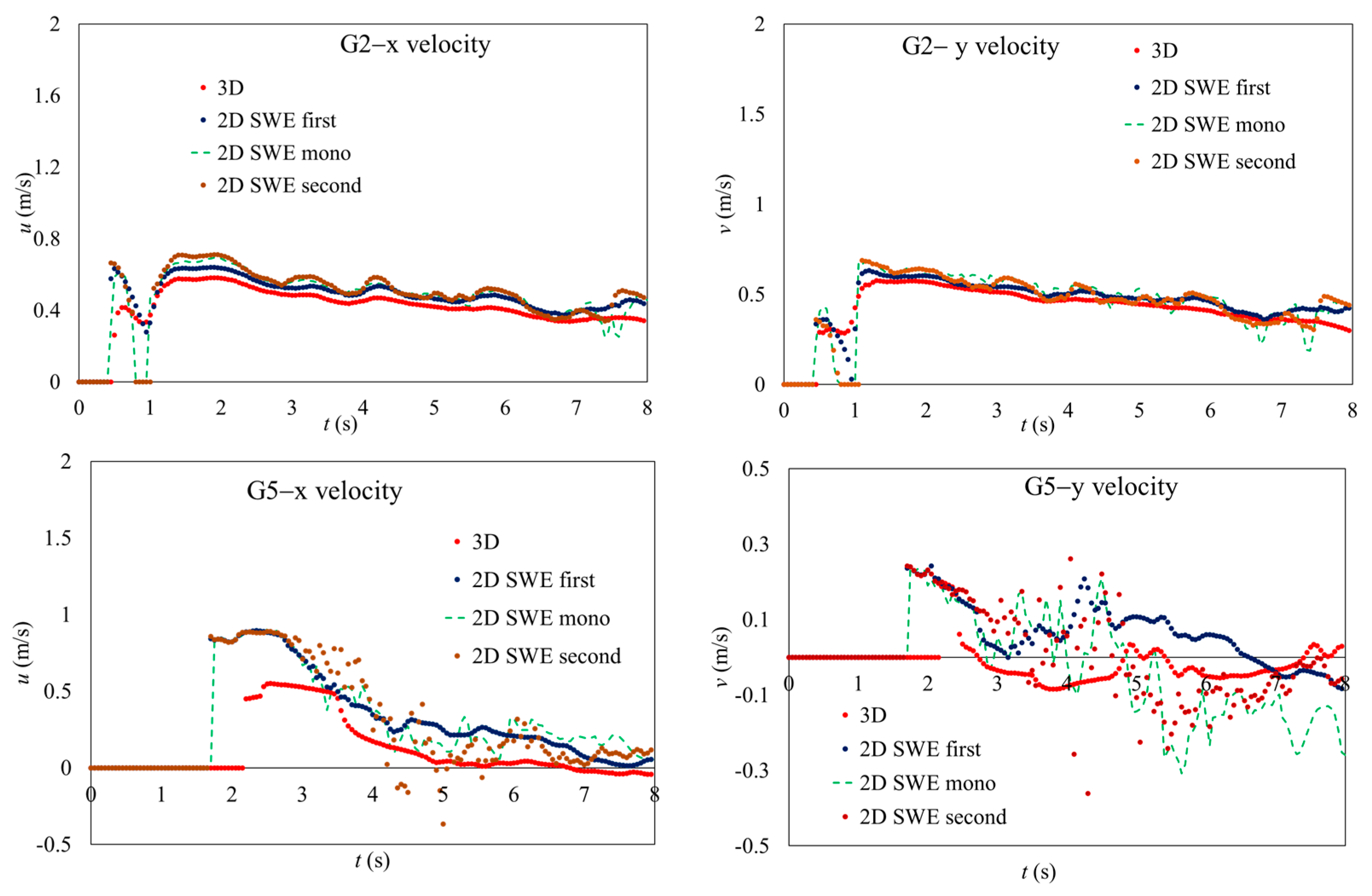
Figure 6.
The aerial view of the inundated map of case A generated by models 4, 5, and 6.
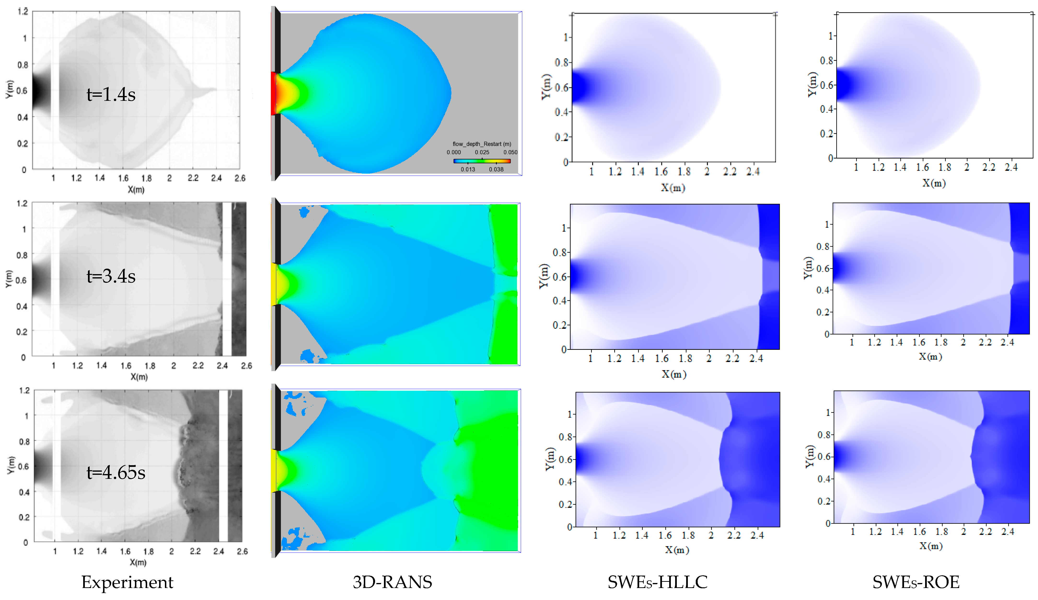
Figure 7.
The stage hydrographs of case A at different gauges were generated by models 4, 5, and 6.

Figure 8.
The aerial view of inundated maps of case B generated by models 1, 2, and 3.

Figure 9.
The aerial view of inundated maps of case B generated by models 4, 5, and 6.

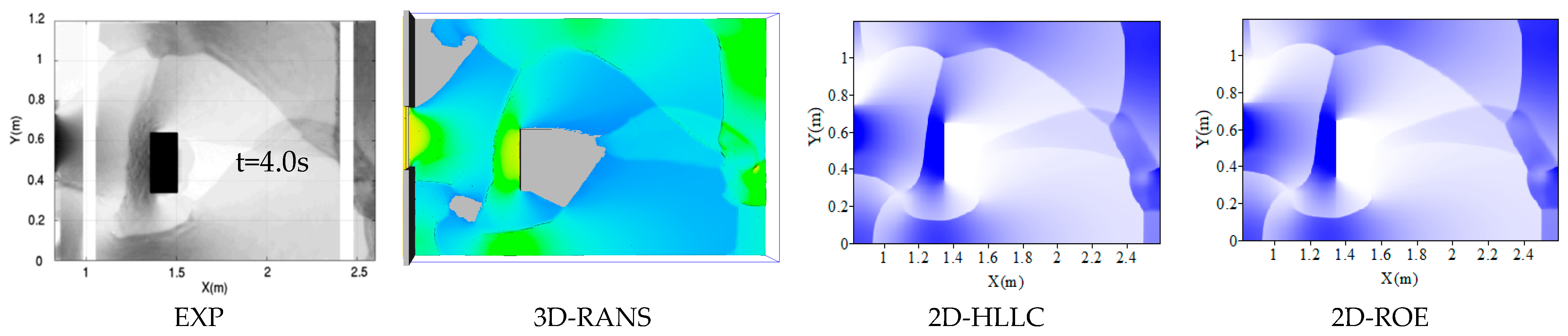
Figure 10.
The stage hydrographs of case B at different gauges as generated by models 1, 2, and 3.

Figure 11.
The stage hydrographs of case B at different gauges as generated by models 4, 5, and 6.

Figure 12.
Location of measured points (dimension in meters).

Figure 13.
Water stage profiles at different gauges.


Table 1.
Mesh convergence analysis.
| No | Cell Size (m) | G1 (mm) | G2 (mm) | G3 (mm) | GCI−G1 (%) | GCI−G2 (%) | GCI−G3 (%) |
|---|---|---|---|---|---|---|---|
| 1 | 0.005 | 18.133 | 5.626 | 26.214 | - | - | - |
| 2 | 0.006 | 18.196 | 5.609 | 25.698 | 0.080 | 0.164 | 0.366 |
| 3 | 0.0072 | 18.601 | 5.551 | 21.706 | 0.513 | 0.550 | 2.884 |
| GCI32/rpGCI21 | 0.997 | 1.003 | 1.02 | ||||
Table 2.
Numerical schemes.
| No | Numerical Schemes | Note | Computational Time | File Size (GB) | ||
|---|---|---|---|---|---|---|
| A | B | A | B | |||
| 1 | 2D-SW model—the first-order accuracy | Flow 3D | 39′08″ | 48′46″ | 9 | 9 |
| 2 | 2D SW model—the second-order accuracy, monotonicity-preserving | Flow 3D | 45′26″ | 52′58″ | 9 | 9 |
| 3 | 2D SW model—the second-order accuracy | Flow 3D | 58′06″ | 1 h 7′24″ | 9 | 9 |
| 4 | 3D model, RANs-RNG turbulence module | Flow 3D | 4 h 00′16″ | 6 h 26′23″ | 93 GB | 97 GB |
| 5 | 2D SWEs-ROE numerical scheme | Proposed model | 9′10″ | 11′13″ | 0.31 | 0.32 |
| 6 | 2D SWEs-HLLC numerical scheme | Proposed model | 9′09″ | 11′05″ | 0.31 | 0.32 |
Table 3.
The relative error (E%) of numerical solutions of the reflected wave in case A.
| Model | 1.4 s | 3.4 s | 4.65 s | |||||||||
|---|---|---|---|---|---|---|---|---|---|---|---|---|
| All | SI | SII | SIII | All | SI | SII | SIII | All | SI | SII | SIII | |
| 1 | 0.05 | - | - | - | 3.50 | 9.02 | 18.37 | 95.43 | 4.80 | 19.20 | 16.00 | 35.60 |
| 2 | 1.21 | - | - | - | 3.50 | 6.02 | 6.12 | 58.55 | 5.30 | 36.20 | 24.80 | 32.40 |
| 3 | 0.28 | - | - | - | 5.02 | 5.26 | 18.37 | 47.49 | 6.30 | 31.90 | 20.40 | 27.60 |
| 4 | 9.32 | - | - | - | 0.94 | 16.24 | 27.96 | 15.89 | 0.60 | 1.00 | 3.40 | 6.50 |
| 5 | 0.44 | - | - | - | 5.09 | 13.78 | 22.45 | 26.25 | 7.70 | 19.10 | 28.30 | 9.10 |
| 6 | 0.44 | - | - | - | 4.65 | 12.10 | 20.00 | 25.00 | 7.93 | 18.99 | 27.89 | 9.49 |
Table 4.
NRMSE value of different numerical schemes in case A.
| Model | G1 | G2 | G3 | G4 | G5 |
|---|---|---|---|---|---|
| 1 | 0.033 | 0.345 | 0.168 | 0.260 | 0.173 |
| 2 | 0.038 | 0.620 | 0.216 | 0.245 | 0.230 |
| 3 | 0.040 | 0.597 | 0.148 | 0.302 | 0.166 |
| 4 | 0.033 | 0.188 | 0.134 | 0.139 | 0.103 |
| 5 | 0.034 | 0.320 | 0.135 | 0.087 | 0.123 |
| 6 | 0.026 | 0.283 | 0.135 | 0.087 | 0.124 |
Table 5.
Relative error (E%) of numerical solutions of the reflected wave in case B.
| No | 1.35s | 2.35s | 4.00s | |||||||||
|---|---|---|---|---|---|---|---|---|---|---|---|---|
| All | SI | SII | SIII | All | SI | SII | SIII | All | SI | SII | SIII | |
| 1 | 4.94 | - | - | - | 4.68 | 35.01 | 7.47 | - | 4.96 | 14.28 | 31.47 | 39.59 |
| 2 | 7.37 | - | - | - | 8.61 | 27.45 | 11.26 | - | 2.88 | 24.99 | 0.398 | 69.20 |
| 3 | 5.17 | - | - | - | 8.77 | 38.41 | 9.17 | - | 4.44 | 33.03 | 39.44 | 48.05 |
| 4 | 16.69 | - | - | - | 4.68 | 2.83 | 10.31 | - | 11.15 | 4.45 | 13.27 | 18.44 |
| 5 | 6.91 | - | - | - | 9.50 | 7.73 | 26.64 | - | 6.10 | 7.05 | 1.04 | 1.72 |
| 6 | 6.92 | - | - | - | 9.42 | 5.88 | 26.09 | - | 6.05 | 7.15 | 0.40 | 1.52 |
Table 6.
NRMSE of numerical results at different gauges in case B.
| Gauges | Models | |||||
|---|---|---|---|---|---|---|
| 1 | 2 | 3 | 4 | 5 | 6 | |
| G1 | 0.169 | 0.157 | 0.151 | 0.169 | 0.190 | 0.180 |
| G2 | 0.424 | 0.506 | 0.462 | 0.177 | 0.161 | 0.145 |
| G3 | 0.352 | 0.460 | 0.437 | 0.169 | 0.218 | 0.224 |
| G4 | 0.362 | 0.331 | 0.364 | 0.245 | 0.248 | 0.246 |
| G5 | 0.099 | 0.134 | 0.135 | 0.114 | 0.156 | 0.152 |
Table 7.
NRMSE of numerical results at different gauges varied with different initial values of c0.
| Model | Model 1 | Model 2 | Model 3 | |||||||
|---|---|---|---|---|---|---|---|---|---|---|
| c0 | 0.70 | 0.99 | 1.21 | 0.70 | 0.99 | 1.21 | 0.70 | 0.99 | 1.21 | |
| Gauges | ||||||||||
| P1 | 0.0064 | 0.0092 | 0.0136 | 0.0157 | 0.0136 | 0.0081 | 0.0212 | 0.0171 | 0.0147 | |
| P2 | 0.0955 | 0.1404 | 0.1076 | 0.0869 | 0.0804 | 0.0622 | 0.1296 | 0.0874 | 0.0555 | |
| P3 | 0.0905 | 0.0983 | 0.0772 | 0.0869 | 0.0804 | 0.0622 | 0.1296 | 0.0874 | 0.0555 | |
| P4 | 0.1327 | 0.0859 | 0.0720 | 0.1431 | 0.0746 | 0.0791 | 0.1454 | 0.1002 | 0.1127 | |
| P5 | 0.1000 | 0.0946 | 0.0627 | 0.1218 | 0.0857 | 0.0734 | 0.1109 | 0.1078 | 0.1014 | |
Disclaimer/Publisher’s Note: The statements, opinions and data contained in all publications are solely those of the individual author(s) and contributor(s) and not of MDPI and/or the editor(s). MDPI and/or the editor(s) disclaim responsibility for any injury to people or property resulting from any ideas, methods, instructions or products referred to in the content. |
© 2023 by the authors. Licensee MDPI, Basel, Switzerland. This article is an open access article distributed under the terms and conditions of the Creative Commons Attribution (CC BY) license (https://creativecommons.org/licenses/by/4.0/).
Share and Cite
MDPI and ACS Style
Hien, L.T.T.; Van Chien, N. A Comparison of Numerical Schemes for Simulating Reflected Wave on Dry and Enclosed Domains. Water 2023, 15, 2781. https://doi.org/10.3390/w15152781
AMA Style
Hien LTT, Van Chien N. A Comparison of Numerical Schemes for Simulating Reflected Wave on Dry and Enclosed Domains. Water. 2023; 15(15):2781. https://doi.org/10.3390/w15152781
Chicago/Turabian StyleHien, Le Thi Thu, and Nguyen Van Chien. 2023. "A Comparison of Numerical Schemes for Simulating Reflected Wave on Dry and Enclosed Domains" Water 15, no. 15: 2781. https://doi.org/10.3390/w15152781
Note that from the first issue of 2016, this journal uses article numbers instead of page numbers. See further details here.