
Understanding the Challenges of Hydrological Analysis at Bridge Collapse Sites

Abstract
:1. Introduction
2. Methods
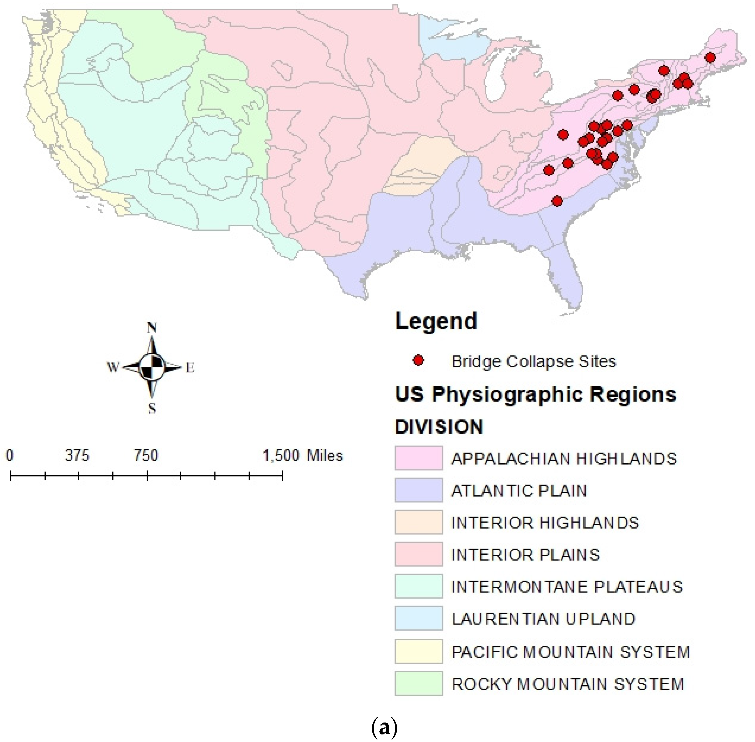
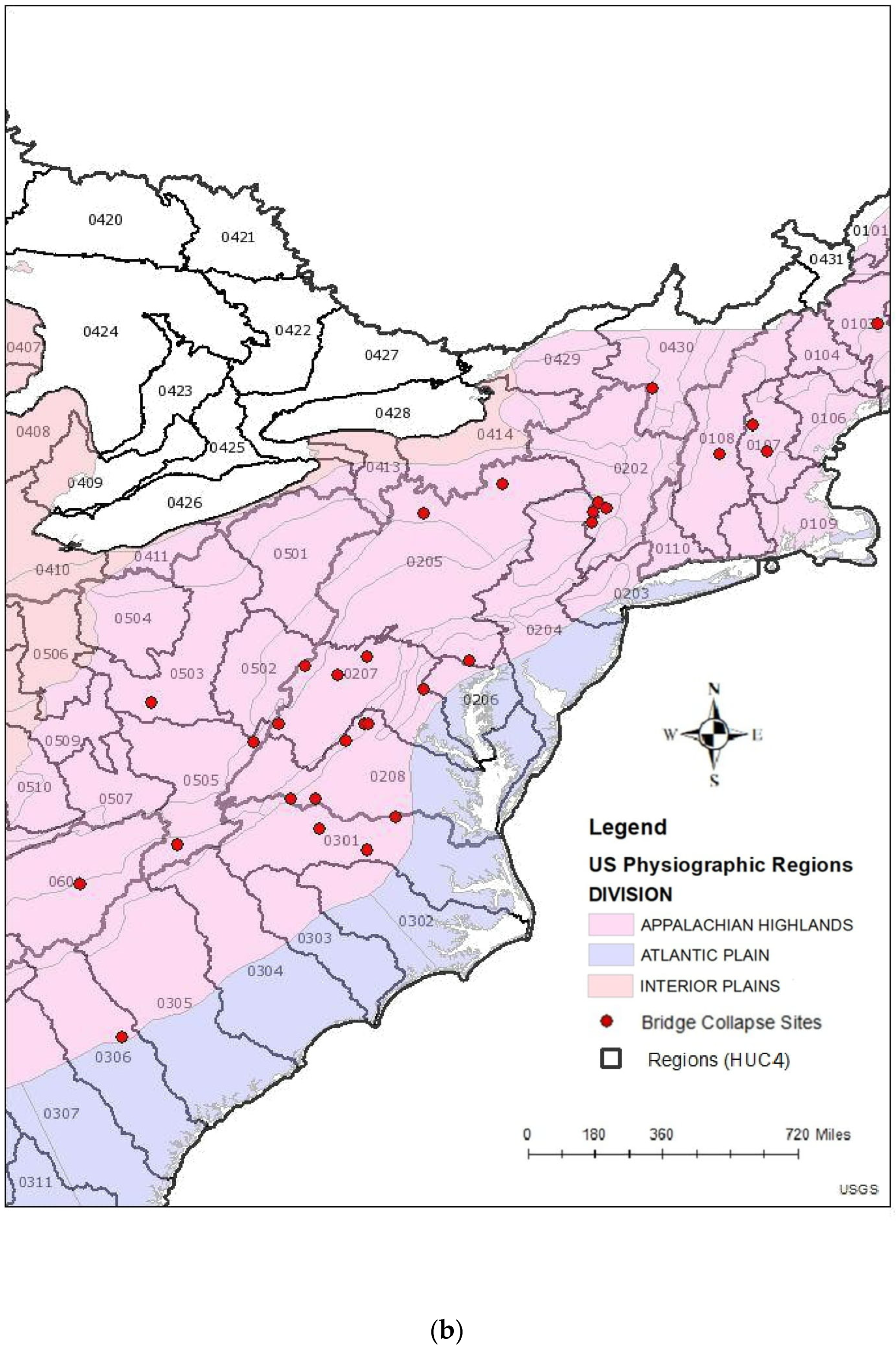
2.1. Selection of Sites
2.2. Analysis of Annual Peak Flow Data
2.3. Analysis of Monthly Flow Data
2.4. Analysis of Predictor Variables
3. Results
3.1. Annual Peak Flows
3.1.1. Best-Fitted with Heavy Tail Distributions
3.1.2. Best-Fitted with Heavy and Light Tail Distributions
3.2. Monthly Flows
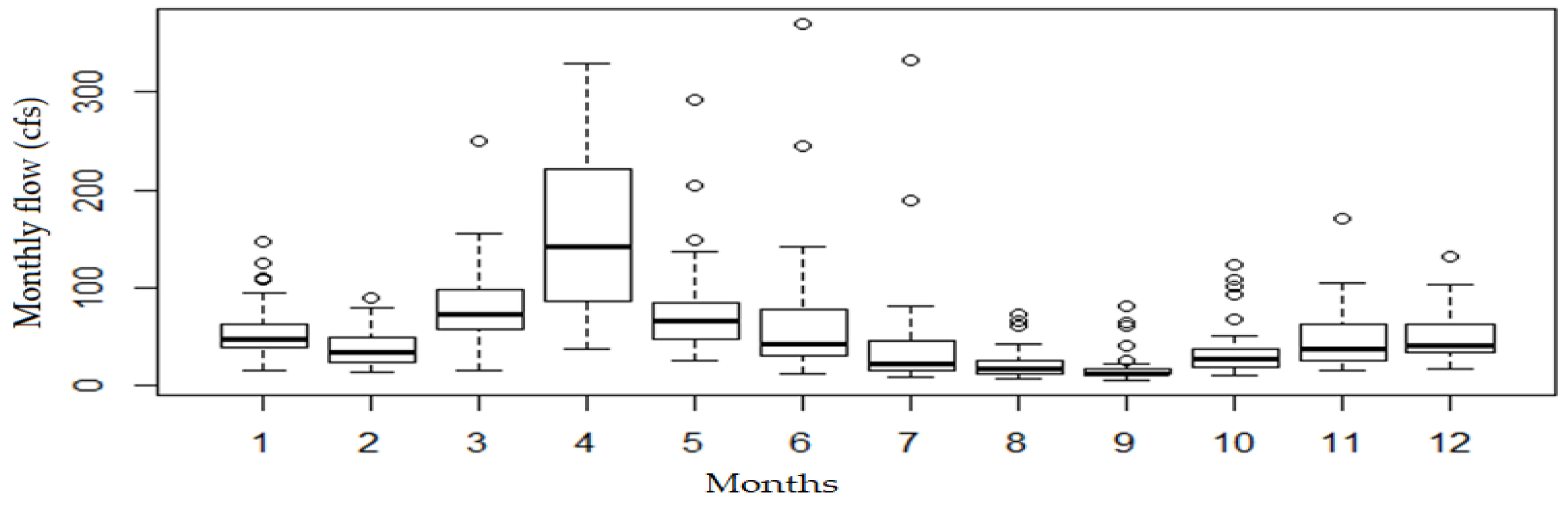
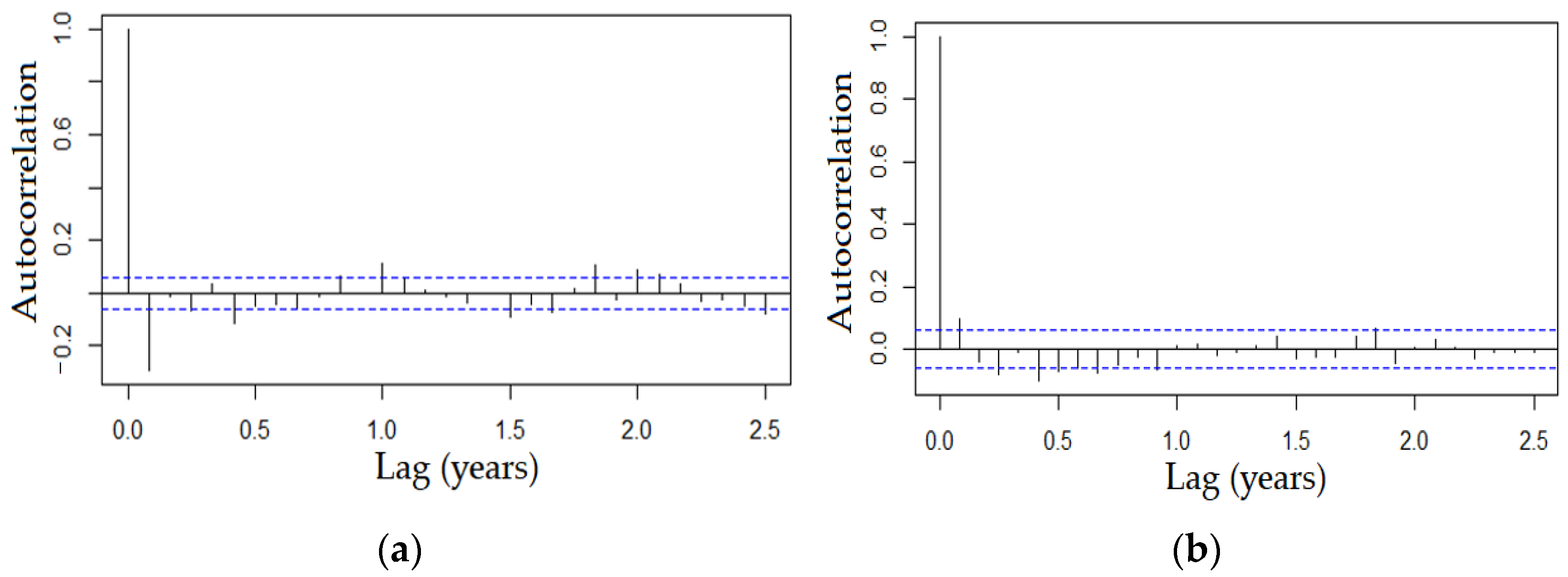
3.2.1. Correlogram and Boxplot
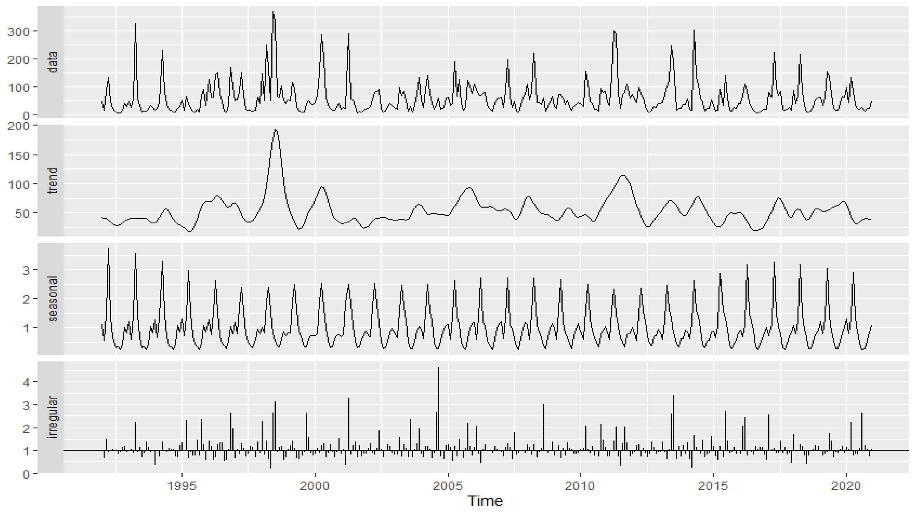
3.2.2. Decomposition
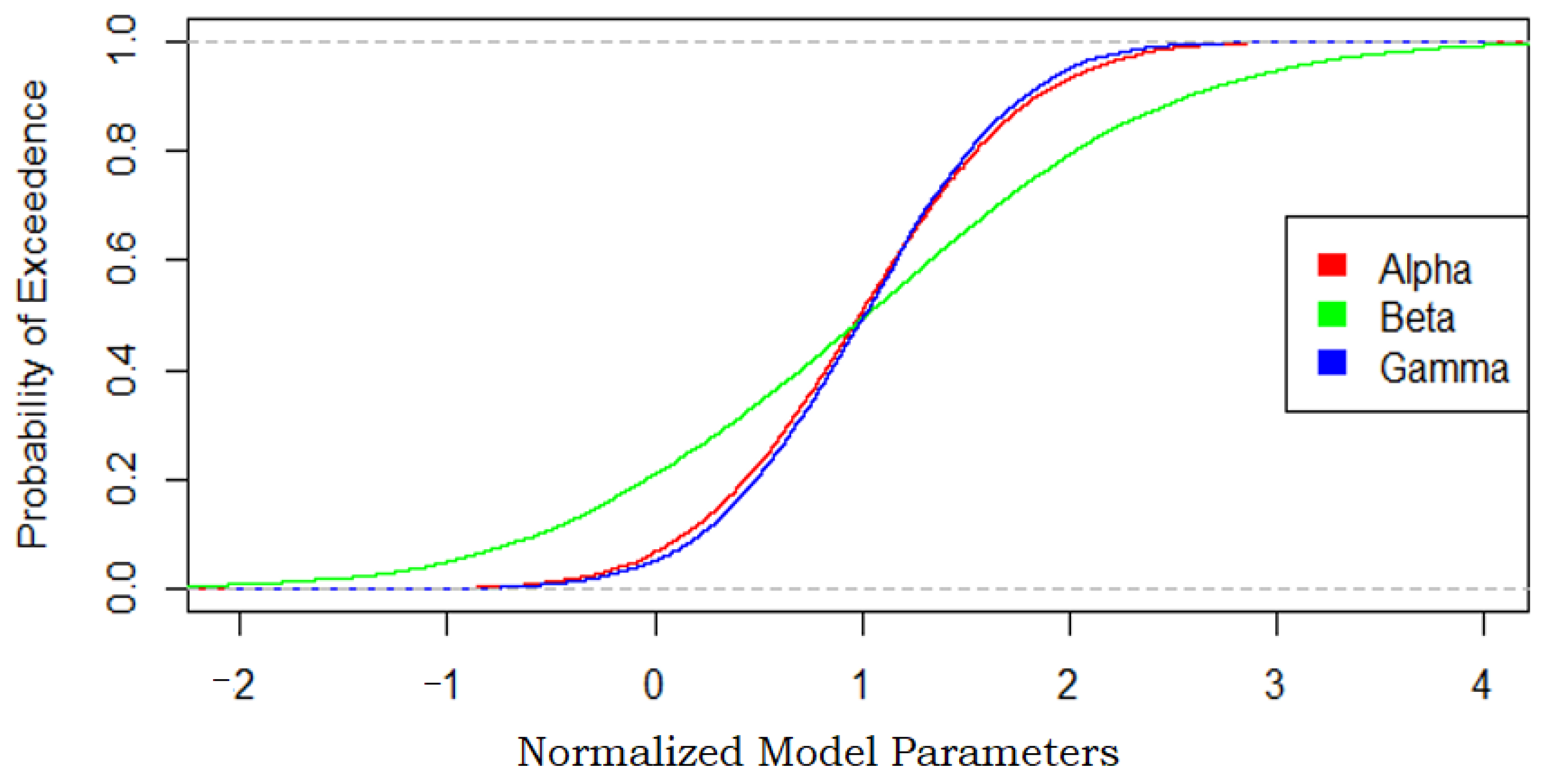
3.2.3. Random Walk and Holt-Winter Models
3.3. Predictor Variables
4. Discussion
- (a)
- Annual peak flow data is best-fit with multiple distributions. For seventeen out of thirty of the collapse sites (56%), the annual peak flow data is best-fitted with multiple distributions. For eleven out of thirty collapse sites (36%), the annual peak flow data is best-fitted with both heavy and light tail distributions with minimum AIC/BIC values, and the goodness-of-fit tests also fail to reject the fitted distributions. Such a finding implies discrepancies or complexity in the dataset studied. It might also suggest that there might be distinct groups or modes within the data, and each group may have its own underlying distribution. Whereas one specific distribution might be reasonable for modeling the central tendency (or concentrated values), another distribution might be more reasonable to model the tail behavior (extreme values). Each best-fitted distribution may help uncover the underlying patterns and provide a more nuanced understanding of the distinct low, medium, and/or high flow values. Finally, site-specific, rigorous investigation is essential, invoking analysis of hydrologic, climatic, geologic, or other hydraulic conditions so that the background physics can be relatively well understood.
- (b)
- There is a discrepancy between the model selection criteria and the goodness-of-fit tests. At about 76% of sites (23 out of 30 sites), the annual peak flow data is best-fitted with a Lognormal distribution with minimum AIC and/or BIC values. However, for all of these sites, the fitted distribution is rejected by the CVM test, whereas for two sites, the distribution is rejected by both the AD and CVM tests. The AIC/BIC and the goodness-of-fit tests are based on different statistical principles and have different underlying assumptions. The AIC/BIC favor models with a high likelihood but implement a penalty for complexity [26,27]. The AD test (a weighted version of the CVM statistic) emphasizes differences near the ends, that is, differences between actual high values and predicted high values [72]. As the Lognormal distribution is not rejected by the AD test, it implies that it can capture the high values relatively well. The CVM statistic is favorable for models regardless of the large-scale or small-scale confidence intervals as retrieved for the shape of the distribution [72]. The CVM statistic also gives equal weight to all observations, including very low and very high values [72]. Therefore, the Lognormal distribution as rejected by the CVM test implies that it cannot capture all observations, including very low and very high values. It is apparent that when the interest is on the tail of the distribution, particularly for heavy tails, adopting certain standard statistical procedures (in reference to the hydraulic design manual) might not be a reasonable choice.
- (c)
- Complex models do not provide significantly better results. For the majority of the sites (87%), a simple model such as Gumbel and/or a Lognormal distribution provides a reasonable fit to the dataset with minimum AIC and/or BIC values. A complex model such as GEV does not improve the fit significantly. Additionally, for GEV, the exact type of enveloped distribution (Gumbel, Weibull, or Frechet) cannot be determined decisively for 40% of the sites (twelve out of thirty). Nonetheless, the diminishing credibility of complex hydrologic models is not acknowledged in current hydraulic design approaches; a number obtained from a complex distribution (i.e., GEV) with no clearly defined physical process seems to be taken with the same consideration as one obtained from a simple model (i.e., Lognormal) with a clearly defined physical process (i.e., multiplicative).
- (d)
- The trend and seasonal variation in the time series data cannot be identified decisively. For monthly flow data, the derived trend does not fit into either a deterministic trend or a random walk trend decisively. Across all sites, the trend is also changing to a wide variety of degrees. For annual peak flow data, no trend is found to be statistically significant at most of the sites. These findings in the preliminary analysis might exclude the collapse sites from further investigation in relation to risk prioritization and resource allocation since linking the collapse risk to the identification of significant positive trends is a common practice in risk studies [17]. Whereas identification of a specific type of trend provides insights into long-term patterns or changes to assess possible changes to collapse risk, the intricacy of pattern recognition in relation to complex hydraulic systems (i.e., debris jams) cannot be performed only using standard trend recognition approaches, at least for the studied collapse sites. In fact, the results of the trend analysis in this study are consistent with other studies in that statistically significant trends were not found at the majority of sites, with mixed results in terms of current trends (positive or negative) [9,35,36,37,38].
- (e)
- Local site characteristics should be considered in relation to fitted distributions. All the studied sites are located within the Appalachian Highland region and are associated with different watersheds. Most of the geospatial characteristics (at the watershed scale) are not significantly different in relation to the comparison of the fitted distributions (i.e., single versus multiple distributions). On the other hand, significantly different characteristics (at the watershed scale) are claimed to be less important in predicting flood behavior [50]. Such a result implies that the spatial scale might need to be narrowed down to identify site-specific differences that lead to specific probabilistic distributions, at least for the studied collapse sites. Recent studies on the collapse sites do reveal specific characteristics for the collapse sites within different physiographic regions, including the Appalachian Highland, such as (a) the presence of very high and very low flows [73], (b) debris jams [45,73], (c) high erosion at bed and bank [45,73], (d) the presence of other in-stream structures [45,73], and (e) the removal of vegetation and other human interference [45]. Such site-specific characteristics are typically included in the hydraulic analysis. In fact, hydraulic analysis is mainly focused on a local scale, whereas hydrologic analysis is mainly focused on a watershed scale. Therefore, rigorous scientific research should be carried out to integrate specific local characteristics within the extreme hydrologic flow analysis, which is commonly performed at the watershed or regional scale.
5. Conclusions
Author Contributions
Funding
Data Availability Statement
Conflicts of Interest
References
- Cook, W.; Barr, P.J.; Halling, M.W. Segregation of Bridge Failure Causes and Consequences. In Proceedings of the Transportation Research Board 93rd Annual Meeting, Washington, DC, USA, 12–16 January 2014. [Google Scholar]
- Nowak, A.S.; Collins, K.R. Reliability of Structures, 2nd ed.; CRC Press: Boca Raton, FL, USA, 2012. [Google Scholar]
- Wardhana, K.; Hadipriono, F.C. Analysis of Recent Bridge Failures in the United States. J. Perform. Constr. Facil. 2003, 17, 144–150. [Google Scholar] [CrossRef] [Green Version]
- Cook, W.; Barr, P.J.; Halling, M.W. Bridge Failure Rate. J. Perform. Constr. Facil. 2013, 29, 4014080. [Google Scholar] [CrossRef]
- Arneson, L.; Zevenbergen, L.; Lagasse, P.; Clopper, P. Evaluating Scour at Bridges, 5th ed.; FHWA: Washington, DC, USA, 2012.
- Kattell, J.; Eriksson, M. Bridge Scour Evaluation: Screening, Analysis, and Countermeasures; Report No. 9877; USDA: Washington, DC, USA, 1998.
- Lee, G.C.; Mohan, S.B.; Huang, C.; Fard, B.N. A Study of U.S. Bridge Failures; MCEER: Buffalo, NY, USA, 2013. [Google Scholar]
- Singh, D.; Tsiang, M.; Rajaratnam, B.; Dienbaugh, N.S. Precipitation extremes over the continental United States in a transient, high-resolution, ensemble climate model experiment. J. Geophys. Res. Atmos. 2013, 118, 7063–7086. [Google Scholar] [CrossRef]
- Milillo, J.M.; Richmond, T.C.; Yohe, G.W. Climate Change Impacts in the United States: The Third National Climate Assessment; US Global Change Research Program: Washington DC, USA, 2014.
- Meyer, M.D.; Flood, M.; Keller, J.; Lennon, J.; McVoy, G.; Dorney, C.; Leonard, K.; Hyman, R.; Smith, J. Strategic Issues Facing Transportation Volume 2: Climate Change, Extreme Weather Events and the Highway System: A Practitioner’s Guide; Report No. 750; NCHRP: Washington, DC, USA, 2013. [Google Scholar]
- Wright, L.; Chinowsky, P.; Strzepek, K.; Jones, R.; Streeter, R.; Smith, J.B.; Mayotte, J.M.; Powell, A.; Jantarasami, L.; Perkins, W. Estimated effects of climate change on flood vulnerability of U.S. bridges. Mitig. Adapt. Strateg. Glob. Chang. 2012, 17, 939–955. [Google Scholar] [CrossRef] [Green Version]
- Neumann, J.E.; Price, J.; Chinowsky, P.; Wright, L.; Ludwig, L.; Streeter, R.; Jones, R.; Smith, J.B.; Perkins, W.; Jantarasami, L.; et al. Climate change risks to US infrastructure: Impacts on roads, bridges, coastal development, and urban drainage. Clim. Chang. 2014, 131, 97–109. [Google Scholar] [CrossRef] [Green Version]
- Meyer, M.D.; Weigel, B. Climate change and transportation engineering: Preparing for a sustainable future. J. Transp. Eng. 2011, 137, 393–403. [Google Scholar] [CrossRef]
- Khelifa, A.; Garrow, L.A.; Higgins, M.J.; Meyer, M.D. Impacts of climate change on scour-vulnerable bridges: Assessment based on HYRISK. J. Infrastruct. Syst. 2013, 19, 138–146. [Google Scholar] [CrossRef] [Green Version]
- Suarez, P.; Anderson, W.; Mahal, V.; Lakshmanan, T.R. Impacts of flooding and climate change on urban transportation: A system wide performance assessment of the Boston Metro Area. Transp. Res. Part D Transp. Environ. 2005, 10, 231–244. [Google Scholar] [CrossRef]
- USDOT Center for Climate Change and Environmental Forecasting. Impacts of Climate Change and Variability on Transportation Systems and Infrastructure: The Gulf Coast Study, Phase 2; Report No. FHWA-HEP-15-004; FHWA: Washington, DC, USA, 2013.
- Flint, M.M.; Fringer, O.; Billington, S.L.; Freyberg, D. Historical analysis of hydraulic bridge collapses in the continental United States. J. Infrastruct. Syst. 2017, 23, 04017005. [Google Scholar] [CrossRef] [Green Version]
- US Code of Federal Regulations. Bridges, Structures and Hydraulics; US Code of Federal Regulations: Washington, DC, USA, 2009. [Google Scholar]
- NYSDOT. Highway Drainage, Highway Design Manual; NYSDOT: Albany, NY, USA, 2014.
- CDOT. Drainage Design Manual; Colorado Department of Transportation: Denver, CO, USA, 2004.
- Eljabri, S.S.M. New Statistical Models for Extreme Values. Ph.D. Thesis, The University of Manchester, Manchester, UK, 2013. [Google Scholar]
- Bailly, F.; Longo, G. Mathematics and the Natural Sciences; Imperial College Press: London, UK, 2011. [Google Scholar]
- D’Espargnat, B. On Physics and Philosophy; Princeton University Press: Oxford, UK, 2002. [Google Scholar]
- Claeskens, G. Statistical model choice. Annu. Rev. Stat. Its Appl. 2016, 3, 233–256. [Google Scholar] [CrossRef]
- Corder, G.W.; Foreman, D.I. Nonparametric Statistics for Non-Statisticians: A Step-by-Step Approach; Wiley: Hoboken, NJ, USA, 2009; ISBN 978-0-470-45461-9. [Google Scholar]
- Akaike, H. Information Theory and an Extension of the Maximum Likelihood Principle. In Selected Papers of Hirotugu Akaike; Parzen, E., Tanabe, K., Kitagawa, G., Eds.; Springer: New York, NY, USA, 1973; pp. 267–281. [Google Scholar] [CrossRef]
- Schwarz Gideon, E. Estimating the dimension of a model. Ann. Stat. 1978, 6, 461–464. [Google Scholar] [CrossRef]
- Babu, G.J.; Feigelson, E.D. Astrostatistics: Goodness of Fit and All That. Astron. Data Anal. Softw. Syst. XV 2006, 351, 127. [Google Scholar]
- Klemes, V. Dilettantism in Hydrology: Transition or Destiny. Water Resour. Res. 1986, 22, 177–188. [Google Scholar] [CrossRef]
- Ario, I.; Yamashita, T.; Tsubaki, R.; Kawamura, S.; Uchida, T.; Watanabe, G.; Fujiwara, A. Investigation of bridge collapse phenomena due to heavy rain floods: Structural, hydraulic, and hydrological analysis. J. Bridge Eng. 2022, 27, 04022073. [Google Scholar] [CrossRef]
- Maddison, B. Scour failure of bridges. Proc. Inst. Civ. Eng.-Forensic Eng. 2012, 165, 39–52. [Google Scholar] [CrossRef]
- Zhang, G.; Liu, Y.; Liu, J.; Lan, S.; Yang, J. Causes and statistical characteristics of bridge failures: A review. J. Traffic Transp. Eng. 2022, 9, 388–406. [Google Scholar] [CrossRef]
- Liu, X.; Ashraf, F.U.; Strom, K.B.; Wang, K.H.; Briaud, J.L.; Sharif, H.; Shafique, S.B. Assessment of the Effects of Regional Channel Stability and Sediment Transport on Roadway Hydraulic Structures: Final Report; Texas Department of Transportation: Austin, TX, USA, 2014.
- Lins, H.; Slack, J. Streamflow trends in the United States. Geophys. Res. Lett. 1999, 26, 227–230. [Google Scholar] [CrossRef] [Green Version]
- Mallakpour, I.; Villarini, G. The changing nature of flooding across the central United States. Nat. Clim. Chang. 2015, 5, 250–254. [Google Scholar] [CrossRef]
- Hirsch, R.M.; Ryberg, K.R. Has the magnitude of floods across the USA changed with global CO2 levels? Hydrol. Sci. J. 2012, 57, 1–9. [Google Scholar] [CrossRef]
- Villarini, G.; Serinaldi, F.; Smith, J.; Krajewski, W.F. On the stationarity of annual flood peaks in the continental United States during the 20th century. Water Resour. Res. 2009, 45, W08417. [Google Scholar] [CrossRef]
- Kundzewicz, Z.W.; Kanae, S.; Seneviratne, S.I.; Handmer, J.; Nicholls, N.; Peduzzi, P.; Mechler, R.; Bouwer, L.M.; Arnell, N.; Mach, K.; et al. Flood risk and climate change: Global and regional perspectives. Hydrol. Sci. J. 2014, 59, 1–28. [Google Scholar] [CrossRef] [Green Version]
- Stewart, B. Measuring What We Manage—The Importance of Hydrological Data to Water Resources Management. In Hydrological Sciences and Water Security: Past, Present, and Future; International Association of Hydrological Sciences: Paris, France, 2014. [Google Scholar]
- Sevruk, B.; Geiger, H. Selection of Distribution Types for Extremes of Precipitation; World Meteorological Organization: Geneva, Switzerland, 1981. [Google Scholar]
- World Meteorological Organization. Statement on the Term Hydrological Normal; Hydrological Coordination Panel: Prague, Czech Republic, 2023; Available online: https://community.wmo.int/activity-areas/hydrology-and-water-resources/hydrological-coordination-panel (accessed on 27 January 2023).
- Bulletin 17B Hydrology Subcommittee. Guidelines for Determining Flood Flow Frequency; USGS Interagency Advisory Committee on Water Data: Reston, VA, USA, 1982.
- England, J.F.; Cohn, T.A.; Faber, B.A.; Stedinger, J.R.; Thomas, W.O.; Veilleux, A.G.; Kiang, J.E.; Mason, R.R. Guidelines for Determining Flood Flow Frequency—Bulletin 17C; U.S. Geological Survey: Reston, VA, USA, 2019.
- Stein, S.; Sedmera, K. Risk-Based Management Guidelines for Scour at Bridges with Unknown Foundations; National Academic Press: Washington, DC, USA, 2007. [Google Scholar]
- Ashraf, F.; Flint, M.M. Retrospective analysis of U.S. hydraulic bridge collapse sites to assess HYRISK performance. In Proceedings of the ASCE World Environmental and Water Resources Congress, Virtual, 7–11 June 2021. [Google Scholar]
- Poórová, J.; Jeneiová, K.; Blaškovičová, L.; Danáčová, Z.; Kotríková, K.; Melová, K.; Paľušová, Z. Effects of the Time Period Length on the Determination of Long-Term Mean Annual Discharge. Hydrology 2023, 10, 88. [Google Scholar] [CrossRef]
- Falcone, J. GAGES-II: Geospatial Attributes of Gages for Evaluating Streamflow; U.S. Geological Survey: Reston, VA, USA, 2011.
- Bloschl, G.; Montanari, A. climate change impacts—Throwing the dice. Hydrol. Process. 2010, 24, 374–381. [Google Scholar] [CrossRef]
- Johnson, P.A. Physiographic Characteristics of Bridge-Stream Intersections. River Res. Appl. 2006, 22, 617–630. [Google Scholar] [CrossRef]
- Ashraf, F.; Tyralis, H.; Papacharalampous, G. Explaining the Flood Behavior for the Bridge Collapse Sites. J. Mar. Sci. Eng. 2022, 10, 1241. [Google Scholar] [CrossRef]
- Gilleland, E.; Katz, R.W. extRemes 2.0: An Extreme Value Analysis Package in R. J. Stat. Softw. 2016, 72, 1–39. [Google Scholar] [CrossRef] [Green Version]
- Webster, V.; Stedinger, J. Log-Pearson Type 3 Distribution and Its Application in Flood Frequency Analysis. I: Distribution Characteristics. J. Hydrol. Eng. 2007, 12, 482–491. [Google Scholar] [CrossRef]
- Coles, S.G. An Introduction to Statistical Modelling of Extreme Values; Springer: London, UK, 2001. [Google Scholar]
- Delignette-Muller, M.L.; Dutang, C. fitdistrplus: An R Package for Fitting Distributions. J. Stat. Softw. 2015, 64, 1–34. [Google Scholar] [CrossRef] [Green Version]
- Saeb, A. Goodness of Fit Test for Continuous Distribution Functions; R Package Version 0.2.0. 2018. Available online: https://cran.r-project.org/web/packages/gnFit/index.html (accessed on 20 January 2023).
- R Core Team. Classical Goodness of Fit Tests for Univariate Distributions; R Package Version 1.2-3. 2022. Available online: https://cran.r-project.org/web/packages/goftest/index.html (accessed on 20 January 2023).
- Pettitt, A. A non-parametric approach to the change-point problem. J. R. Stat. Soc. Ser. C 1979, 28, 126–135. [Google Scholar] [CrossRef]
- Mann, H.B. Nonparametric tests against trend. Econ. J. Econ. Soc. 1945, 13, 245–259. [Google Scholar] [CrossRef]
- Pohlert, T. Trend: Non-Parametric Trend Tests and Change-Point Detection; R Package Version 1.1.2. 2020. Available online: https://cran.r-project.org/web/packages/trend/index.html (accessed on 20 January 2023).
- McLeod, A.I. Trend: Non-Parametric Trend Tests and Change-Point Detection; R Package Version 2.2.1. 2022. Available online: https://cran.r-project.org/web/packages/Kendall/index.html (accessed on 20 January 2023).
- Dagum, E.B.; Bianconcini, S. Seasonal Adjustment Methods and Real Time Trend-Cycle Estimation, 1st ed.; Springer: Berlin, Germany, 2016. [Google Scholar]
- Sax, C.; Eddelbuettel, D. R Interface to X-13-ARIMA-SEATS; R Package Version 1.9.0. 2022. Available online: https://cran.r-project.org/web/packages/seasonal/index.html (accessed on 20 January 2023).
- Cowpertwait, P.S.P.; Metcalfe, A. Introductory Time Series with R; Springer: Berlin, Germany, 2009. [Google Scholar] [CrossRef]
- Scheer, J. Failed Bridges: Case Studies, Causes and Consequences; Wiley: Hoboken, NJ, USA, 2010. [Google Scholar] [CrossRef]
- Czapiga, M.J.; Smith, V.B.; Nittrouer, J.A.; Mohrig, D.; Parker, G. Internal connectivity of meandering rivers: Statistical generalization of channel hydraulic geometry. Water Resour. Res. 2015, 51, 7485–7500. [Google Scholar] [CrossRef] [Green Version]
- Kim, T.K. T test as a parametric statistic. Korean J. Anesthesiol. 2015, 68, 540–546. [Google Scholar] [CrossRef] [PubMed] [Green Version]
- Nair, J.; Wierman, A.; Zwart, B. The Fundamentals of Heavy Tails: Properties, Emergence, and Estimation (Cambridge Series in Statistical and Probabilistic Mathematics); Cambridge University Press: Cambridge, UK, 2022. [Google Scholar] [CrossRef]
- Stephens, M.A. EDF Statistics for Goodness of Fit and Some Comparisons. J. Am. Stat. Assoc. 1974, 69, 730–737. [Google Scholar] [CrossRef]
- Laio, F. Cramer–von Mises and Anderson-Darling goodness of fit tests for extreme value distributions with unknown parameters. Water Resour. Res. 2004, 40. [Google Scholar] [CrossRef]
- Klemes, V. Scientific Basis of Water Resource Management; National Academy Press: Washington, DC, USA, 1982. [Google Scholar]
- Myers, D.T.; Ficklin, D.L.; Robeson, S.M.; Neupane, R.P.; Botero-Acosta, A.; Avellaneda, P.M. Choosing an arbitrary calibration period of hydrologic models: How much does it influence water balance simulations? Hydrol. Process. 2021, 35, e14045. [Google Scholar] [CrossRef]
- Babu, G.J.; Toreti, A. A Goodness-of- fit test for heavy tailed distributions with unknown parameters and its application to simulated precipitation extremes in the Euro-Mediterranean region. J. Stat. Plan. Inference 2016, 174, 11–19. [Google Scholar] [CrossRef]
- Ashraf, F.; Spaunhorst, M. At a station hydraulic geometry for reaches with bridge collape events. River Res. Appl. 2023, 39, 108–121. [Google Scholar] [CrossRef]


| Site Number | USGS Station (Number of Observations) | USGS Station Name | Location | Hydrologic Unit Code | Drainage Area (Square Miles) | Period for the Flow Record | Range of Flows (cfs) | Maximum Flow Year | Collapsed Bridge ID and Type (from the NYSDOT) | Life Span of the Collapsed Bridge | Collapse Type | Collapse Cause |
|---|---|---|---|---|---|---|---|---|---|---|---|---|
| 1 | 01606500 (96) | South Branch Potomac River near Petersburg, West Virginia | Grant County, West Virginia | 02070001 | 1684.5 | 1929–2022 (93 years) | 4660–130,000 | 1986 | 56 Concrete-box beam | NA–1993 | NA | Hydraulic Flood |
| 2 | 01663500 (73) | Hazel River at Rixeyville, Virginia | Culpeper County, Virginia | 02080103 | 739.3 | 1942–2022 (80 years) | 2670–60,000 | 1943 | 1038 Steel-beam | NA–1979 | NA | Hydraulic Scour |
| 3 | 01154000 (64) | Saxtons River at Saxtons River, Vermont | Windham County, Vermont | 01080107 | 187.3 | 1941–2022 (81 years) | 821–21,600 | 2011 | 77 Steel-stringer | 1935–1995 | Partial collapse | Hydraulic |
| 4 | 02064000 (85) | Falling River near Naruna, Virginia | Campbell County, Virginia | 03010102 | 165 | 1942–2022 (80 years) | 888–62,800 | 1996 | 1397 Steel-corrugated pipe | NA–1995 | NA | Hydraulic Scour |
| 5 | 02026000 (84) | James River at Bent Creek, Virginia | Nelson County, Virginia | 02080203 | 3649 | 1925–2022 (97 years) | 7060–226,000 | 1986 | 190 Steel-girder | 1952–1996 | Total collapse | Hydraulic Flood |
| 6 | 03164000 (92) | New River near Galax, Virginia | Grayson County, Virginia | 05050001 | 2952.7 | 1930–2022 (92 years) | 6200–141,000 | 1940 | 1401 Steel-beam | 1932–1995 | NA | Hydraulic Debris |
| 7 | 01662800 (62) | Battle Run near Laurel Mills, Virginia | Rappahannock County, Virginia | 02080103 | 66.7 | 1959–2022 (63 years) | 227–9120 | 1977, 1995 | 136 Steel-beam | NA–2004 | Total collapse | Hydraulic |
| 8 | 01665500 (77) | Rapidan River near Ruckersville, Virginia | Madison County, Virginia | 02080103 | 296.6 | 1943–2022 (79 years) | 735–106,000 | 1995 | 189 Steel-beam | NA–1996 | Total collapse | Hydraulic |
| 9 | 01611500 (100) | Cacapon River near Great Cacapon, West Virginia | Morgan County, West Virginia | 02070003 | 1748.5 | 1923–2022 (99 years) | 1950–87,600 | 1936 | 42 Steel-culvert | NA–1996 | NA | Hydraulic Flood |
| 10 | 02046000 (77) | Stony Creek near Dinwiddie, Virginia | Dinwiddie County, Virginia | 03010201 | 288.5 | 1947–2022 (75 years) | 330–11,400 | 1973 | 1726 Steel-corrugated pipe | 1971–2003 | Total collapse | Hydraulic Washout |
| 11 | 01349810 (25) | West Kill near West Kill, New York | Greene County, New York | 02020005 | 73.7 | 1996–2022 (26 years) | 413–19,100 | 2011 | 1406 Steel-multi grid | 1940–1996 | Total collapse | Hydraulic |
| 12 | 01525981 (33) | Tuscarora Creek above South Addison, New York | Steuben County, New York | 02050104 | 261.9 | 1989–2022 (33 years) | 2190–27,400 | 2021 | 1379 Steel-truss | 1962–1994 | Partial collapse | Hydraulic Flood |
| 13 | 01362198 (26) | Esopus Creek at Shandaken, New York | Ulster County, New York | 02020006 | 154.1 | 1964–1988 (24 years) | 1000–16,100 | 1987 | 3611 Steel-girder | 1903–2011 | Total collapse | Hydraulic Flood |
| 14 | 03465500 (103) | Nolichucky River at Embreeville, Tennessee | Washington County, Tennessee | 06010108 | 2081.6 | 1921–2022 (101 years) | 5690–110,000 | 1978 | 1634 Steel-beam | NA–2001 | Partial collapse | Hydraulic Flood |
| 15 | 01644000 (97) | Goose Creek near Leesburg, Virginia | Loudoun County, Virginia | 02070008 | 859.2 | 1930–2022 (92 years) | 1300–78,100 | 1972 | 378 NA | 1920–1971 | NA | Hydraulic |
| 16 | 03182500 (93) | Greenbrier River at Buckeye, West Virginia | Pocahontas County, West Virginia | 05050003 | 1365.0 | 1930–2022 (92 years) | 5630–82,000 | 1986 | 57 Concrete-box beam | NA–1996 | NA | Hydraulic Flood |
| 17 | 01596500 (74) | Savage River near Barton, Maryland | Garrett County, Maryland | 02070002 | 124.7 | 1949–2022 (73 years) | 415–7510 | 1955 | 1482 Steel-stringer | 1940–1996 | Partial collapse | Hydraulic Flood |
| 18 | 04273800 (30) | Little Ausable River near Valcour, New York | Clinton County, New York | 04150408 | 1992–2022 (30 years) | 184–7210 | 1998 | 249 Steel-Jack Arch | 1940–2011 | Total collapse | Hydraulic Flood, Scour | |
| 19 | 02024915 (19) | Pedlar River at Forest Road near Buena Vista, Virginia | Amherst County, Virginia | 02080203 | 71.0 | 2004–2022 (18 years) | 150–2760 | 2006 | 1402 Steel-beam | 1932–1995 | NA | Hydraulic Debris |
| 20 | 01086000 (63) | Warner River at Davisville, New Hampshire | Merrimack County, New Hampshire | 01070003 | 381.6 | 1999–2022 (23 years) | 1440–8640 | 2006 | 801 Concrete | NA–1987 | NA | Hydraulic Scour |
| 21 | 03159540 (57) | Shade River near Chester Ohio | Meigs County, Ohio | 05030202 | 400.9 | 1966–2022 (56 years) | 954–15,600 | 1997 | 31 Steel-truss pony | NA–1998 | NA | Hydraulic Flood |
| 22 | 02079640 (57) | Allen Creek near Boydton, Virginia | Mecklenburg County, Virginia | 03010106 | 138.8 | 1962–2022 (60 years) | 541–7380 | 2003 | 137 Aluminum- box culvert | 2000–2006 | Total collapse | Hydraulic Washout |
| 23 | 01365000 (85) | Rondout Creek near Lowes Corners New York | Sullivan County, New York | 02020007 | 99.6 | 1937–2021 (84 years) | 612–8200 | 2011 | 1631 Steel-girder | 1955–2005 | Partial collapse | Hydraulic Scour |
| 24 | 01510000 (79) | Otselic River at Cincinnatus New York | Cortland County, New York | 02050102 | 383.0 | 1939–2022 (83 years) | 1820–8390 | 1943 | 828 NA | NA–1973 | Partial collapse | Hydraulic Agnes |
| 25 | 01362370 (28) | Stony Clove Creek Blw Ox Clove at Chichester New York | Ulster County, New York | 02020006 | 80.2 | 1997–2022 (25 years) | 333–14,300 | 2011 | 3627 Steel-girder | 1968–2011 | Total collapse | Hydraulic Scour |
| 26 | 02196000 (78) | Stevens Creek near Modoc, South Carolina | Edgefield County, South Carolina | 03060107 | 1408.4 | 1940–2022 (82 years) | 2080–35,100 | 1940 | 992 (Concrete-girder) | 1975–1977 | NA | Hydraulic Flood |
| 27 | 01613525 (18) | Licking Creek at Pectonville, Maryland | Washington County, Maryland | 02070004 | 502.1 | 2005–2022 (17 years) | 2280–8590 | 2005 | 1484 Steel-stringer | 1950–1996 | Partial collapse | Hydraulic Flood |
| 28 | 01580000 (96) | Deer Creek at Rocks, Maryland | Harford County, Maryland | 02050306 | 244.4 | 1927–2022 (95 years) | 332–13,600 | 1933 | 407 Steel-beam | NA–1972 | NA | Hydraulic Agnes |
| 29 | 01091000 (54) | South Branch Piscataquog River near Goffstown, New Hampshire | Hillsborough County, New Hampshire | 01070002 | 266.8 | 1941–2021 (80 years) | 615–8800 | 2007 | 799 Concrete | NA–1987 | NA | Hydraulic Scour |
| 30 | 01046000 (49) | Austin Stream at Bingham, Maine | Somerset County, Maine | 01030003 | 243.2 | 1932–2022 (90 years) | 1050–8280 | 1967 | 1547 Concrete-slab | 1957–1987 | Partial collapse | Hydraulic Flood |
| Site Number (in Reference to Table 1) | Shape Parameter from GEV (Confidence Interval) | p Values for the Log-Likelihood Test (GEV and Gumbel) |
Minimum AIC/BIC | p Values for the AD/CVM Test for GEV | Mann-Kendall Trend (Tao/p) |
|---|---|---|---|---|---|
| 1 | 0.5 (0.25–0.73) | 4.3 × 10⁻¹¹ | 2008/2016 | 0.65/0.72 | 0.04/0.57 |
| 2 | 0.6 (0.3–0.85) | 4.2 × 10⁻⁹ | 1441/1447 | 0.48/0.61 | 0.07/0.39 |
| 3 | 0.3 (0.15–0.5) | 2.0 × 10⁻⁶ | 1059/1065 | 0.49/0.56 | 0.09/0.32 |
| 4 | 0.4 (0.23–0.58) | 2.2 × 10⁻¹² | 1605/1612 | 0.41/0.42 | 0.06/0.46 |
| Site Number (in Reference to Table 1) | Shape Parameter from GEV (Confidence Interval) | p Values for the Log-Likelihood Test (GEV and Gumbel) |
Minimum AIC/BIC | p Values for the AD/CVM Test for Lognormal | p Values for the AD/CVM Test for GEV | Mann-Kendall Trend (Tao/p) |
|---|---|---|---|---|---|---|
| 5 | 0.33 (0.1–0.5) | 1.5 × 10⁻⁹ | 1582/1587 | 0.27/<2 × 10−16 | 0.4/0.4 | 0.11/0.16 |
| 6 | 0.29 (0.08–0.5) | 2.8 × 10⁻⁵ | 1995/2001 | 0.39/<2 × 10−16 | 0.31/0.19 | 0.08/0.27 |
| 7 | 0.70 (0.34–0.9) | 1.1 × 10⁻⁷ | 1052/1057 | 0.06/<2 × 10−16 | 0.26/0.24 | 0.23/0.01 |
| 8 | 0.63 (0.35–0.9) | 3.2 × 10⁻¹³ | 1511/1515 | 0.42/<2 × 10−16 | 0.74/0.63 | 0.2/0.01 |
| 9 | 0.30 (0.11–0.5) | 2.6 × 10⁻⁶ | 2093/2098 | 0.32/<2 × 10−16 | 0.56/0.73 | −0.05/0.51 |
| 10 | 0.48 (0.3–0.7) | 1.1 × 10⁻⁶ | 1329/1334 | 0.13/<2 × 10−16 | 0.34/0.28 | −0.03/0.73 |
| 11 | 0.35 (0.04–0.7) | 0.003 | 453/455 | 0.49/<2 × 10−16 | 0.89/0.93 | −0.13/0.39 |
| 12 | 0.27 (−0.03–0.6) | 0.03 | 638/641 | 0.46/<2 × 10−16 | 0.79/0.73 | −0.2/0.11 |
| 13 | 0.48 (−0.07–1) | 0.01 | 496/499 | 0.46/<2 × 10−16 | 0.5/0.58 | 0.15/0.31 |
| Site Number (in Reference to Table 1) | Shape Parameter from GEV (Confidence Interval) | p
Values for the Log-Likelihood Test (GEV and Gumbel) |
Minimum AIC/BIC | p Values for the AD/CVM Test for Lognormal | p Values for the AD/CVM Test for GEV | Mann-Kendall Trend (Tao/p) |
|---|---|---|---|---|---|---|
| 14 | 0.32 (0.1–0.5) | 1 × 10⁻⁶ | 2231/2236 (Lognormal) | 0.16/<2 × 10−16 | 0.32/0.25 | 0.10/0.12 |
| 2229/2237 (GEV) | ||||||
| 15 | 0.38 (0.2–0.5) | 3 × 10⁻¹¹ | 1942/1947 (Lognormal) | 0.004/<2 × 10−16 | 0.03/0.03 | 0.08/0.25 |
| 1940/1948 (GEV) | ||||||
| 16 | 0.14 (0.02–0.3) | 0.005 | 1918/1923 (Lognormal) | 0.13/<2 × 10−16 | 0.47/0.46 | 0.14/0.05 |
| 1917/1925 (GEV) | ||||||
| 17 | 0.14 (0.02–0.3) | 0.001 | 1189/1194 (Lognormal) | 0.1/<2 × 10−16 | 0.67/0.83 | 0.05/0.50 |
| 1188/1195 (GEV) | ||||||
| 18 | 0.47 (0.1–0.8) | 3.5 × 10⁻⁵ | 472/474 (Lognormal) | 0.35/<2 × 10−16 | 0.93/0.88 | −0.3/0.04 |
| 471/476 (GEV) |
| Site Number (in Reference to Table 1) | Shape Parameter from GEV (Confidence Interval) | p Values for the Log-Likelihood Test (GEV and Gumbel) | Well-Fitted Distributions | AIC/BIC Values | p Values for the AD/CVM Test | Mann-Kendall Trend (Tao/p) |
|---|---|---|---|---|---|---|
| 19 | 0.13 (−0.2–0.5) | 0.44 | Gumbel | 279/281 | 0.76/0.82 | 0.03/0.88 |
| Weibull | 280/281 | 0.43/0.3 | ||||
| Lognormal | 280/282 | 0.3/<2 × 10−16 | ||||
| 20 | 0.13 (−0.02–0.3) | 0.06 | GEV | 1049/1056 | 0.39/0.41 | 0.05/0.53 |
| Gumbel | 1056/1051 | 0.09/0.14 | ||||
| Lognormal | 1050/1054 | 0.13/<2 × 10−16 | ||||
| 21 | 0.09 (−0.03–0.2) | 0.11 | GEV | 1004/1010 | 0.05/0.11 | 0.11/0.23 |
| Gumbel | 1004/1008 | 0.01/0.04 | ||||
| Lognormal | 1005/1009 | 0.01/<2 × 10−16 | ||||
| 22 | 0.07 (−0.2–0.3) | 0.39 | Gumbel | 966/970 | 0.93/0.96 | 0.04/0.7 |
| Lognormal | 966/970 | 0.65/<2 × 10−16 | ||||
| 23 | 0.16 (−0.06–0.4) | 0.10 | GEV | 1034/1040 | 0.48/0.76 | 0.05/0.47 |
| Gumbel | 1035/1039 | 0.12/0.21 | ||||
| Lognormal | 1034/1038 | 0.48/<2 × 10−16 | ||||
| 24 | −0.01 (−0.2–0.2) | 1.00 | Gumbel | 1389/1393 | 0.99/0.99 | −0.1/0.07 |
| Lognormal | 1388/1393 | 0.85/<2 × 10−16 | ||||
| 25 | 0.19 (−0.2–0.61) | 0.27 | Weibull | 534/536 | 0.65/0.52 | −0.3/0.05 |
| Gumbel | 537/539 | |||||
| 26 | −0.04 (−0.2–0.1) | 0.63 | Gumbel | 1583/1587 | 0.69/0.78 | −0.1/0.2 |
| Weibull | 1583/1588 | 0.66/0.7 | ||||
| 27 | −0.32 (−0.7–0.1) | 0.21 | Gumbel | 306/308 | 0.69/0.78 | −0.3/0.15 |
| Weibull | 305/306 | 0.98/0.97 | ||||
| Lognormal | 306/308 | 0.51/<2 × 10−16 | ||||
| 28 | 0.12 (−0.01–0.3) | 0.08 | GEV | 1718/1726 | 0.06/0.05 | −0.04/0.54 |
| Gumbel | 1719/1724 | 0.002/0.002 | ||||
| 29 | 0.15 (−0.06–0.4) | 0.10 | GEV | 915/921 | 0.72/0.73 | 0.1/0.3 |
| Gumbel | 915/919 | 0.76/0.93 | ||||
| Lognormal | 913/917 | 0.59/<2 × 10−16 | ||||
| 30 | 0.21 (−0.1–0.6) | 0.12 | Gumbel | 844/850 | 0.03/0.76 | |
| Lognormal | 842/846 | 0.52/<2 × 10−16 |
| Site Number (in Reference to Table 1) | ADF Test (p Value) | Significant Values at Significant Lags | % of MAXIMUM Linear Dependency (RW Model) | HW Model Alpha (α) | HW Model Beta (β) | HW Model Gamma (γ) | % of Maximum Linear Dependency (HW Model) |
|---|---|---|---|---|---|---|---|
| 1 | Stationary (p < 0.01) | 0.49 (Lag 0.1) | 7.8% | 0.17 | 0.009 | 0.08 | 1.96% |
| −0.31 (Lag 0.5) | |||||||
| 0.29 (Lag 1) | |||||||
| 2 | Stationary (p < 0.01) | 0.5 (Lag 0.1) | 7.8% | 0.21 | 0 | 0.04 | 3.61% |
| −0.18 (Lag 0.5) | |||||||
| 0.21 (Lag 1) | |||||||
| 3 | Stationary (p < 0.01) | 0.38 (Lag 0.1) | 16% | 0.07 | 0.02 | 0.16 | 0% |
| −0.19 (Lag 0.5) | |||||||
| 0.65 (Lag 1) | |||||||
| 4 | Stationary (p < 0.01) | 0.43 (Lag 0.1) | 13.7% | 0.19 | 0 | 0.1 | 0.81% |
| Not significant | |||||||
| 0.21 (Lag 1) | |||||||
| 5 | Stationary (p < 0.01) | 0.43 (Lag 0.1) | 9.6% | 0.28 | 0.003 | 0.09 | 0.81% |
| −0.12 (Lag 0.5) | |||||||
| 0.15 (Lag 1) | |||||||
| 6 | Stationary (p < 0.01) | 0.55 (Lag 0.1) | 8.4% | 0.35 | 0 | 0.11 | 1% |
| −0.11 (Lag 0.5) | |||||||
| 0.27 (Lag 1) | |||||||
| 7 | Stationary (p < 0.01) | 0.48 (Lag 0.1) | 9% | 0.24 | 0.005 | 0.10 | 2.56% |
| −0.17 (Lag 0.5) | |||||||
| 0.28 (Lag 1) | |||||||
| 8 | Stationary (p < 0.01) | 0.48 (Lag 0.1) | 9% | 0.17 | 0 | 0.05 | 3.6% |
| Not significant | |||||||
| 0.13 (Lag 1) | |||||||
| 9 | Stationary (p < 0.01) | 0.48 (Lag 0.1) | 3.6% | 0.27 | 0.008 | 0.37 | 3.6% |
| Not significant | |||||||
| 0.13 (Lag 1) | |||||||
| 10 | Stationary (p < 0.01) | 0.53 (Lag 0.1) | 9% | 0.38 | 0 | 0.08 | 1.69% |
| −0.11 (Lag 0.5) | |||||||
| 0.22 (Lag 1) | |||||||
| 11 | Stationary (p < 0.01) | 0.29 (Lag 0.1) | 7.3% | 0.07 | 0.01 | 0.16 | 4% |
| Not significant | |||||||
| 0.21 (Lag 1) | |||||||
| 12 | Stationary (p < 0.01) | 0.37 (Lag 0.1) | 9% | 0.03 | 0 | 0.19 | 0% |
| −0.16 (Lag 0.5) | |||||||
| 0.26 (Lag 1) | |||||||
| 13 | Stationary (p < 0.01) | 0.37 (Lag 0.1) | 9% | 0.07 | 0.009 | 0.09 | 0% |
| −0.17 (Lag 0.5) | |||||||
| 0.46 (Lag 1) | |||||||
| 14 | Stationary (p < 0.01) | 0.53 (Lag 0.1) | 9% | 0.21 | 0.002 | 0.09 | 0.81% |
| −0.22 (Lag 0.5) | |||||||
| 0.39 (Lag 1) | |||||||
| 15 | Stationary (p < 0.01) | 0.48 (Lag 0.1) | 11.56% | 0.31 | 0.001 | 0.07 | 1% |
| −0.13 (Lag 0.5) | |||||||
| 0.21 (Lag 1) | |||||||
| 16 | Stationary (p < 0.01) | 0.48 (Lag 0.1) | 8.4% | 0.11 | 0.01 | 0.08 | 1% |
| −0.43 (Lag 0.5) | |||||||
| 0.49 (Lag 1) | |||||||
| 17 | Stationary (p < 0.01) | 0.45 (Lag 0.1) | 9% | 0.18 | 0 | 0.07 | 1% |
| −0.36 (Lag 0.5) | |||||||
| 0.48 (Lag 1) | |||||||
| 18 | Stationary (p < 0.01) | 0.41 (Lag 0.1) | 9% | 0.19 | 0.007 | 0.21 | 3.24% |
| Not significant | |||||||
| 0.32 (Lag 1) | |||||||
| 19 | Stationary (p < 0.01) | 0.65 (Lag 0.1) | 4% | 0.35 | 0 | 0.31 | 4% |
| −0.17 (Lag 0.5) | |||||||
| 0.25 (Lag 1) | |||||||
| 20 | Stationary (p < 0.01) | 0.37 (Lag 0.1) | 8.4% | 0.11 | 0.03 | 0.06 | 4% |
| −0.11 (Lag 0.5) | |||||||
| 0.37 (Lag 1) | |||||||
| 21 | Stationary (p < 0.01) | 0.38 (Lag 0.1) | 14.4% | 0.07 | 0.01 | 0.18 | 0.09% |
| −0.34 (Lag 0.5) | |||||||
| 0.35 (Lag 1) | |||||||
| 22 | Stationary (p < 0.01) | 0.48 (Lag 0.1) | 11.56% | 0.18 | 0.01 | 0.13 | 1.69% |
| Not significant | |||||||
| Not significant | |||||||
| 23 | Stationary (p < 0.01) | 0.37 (Lag 0.1) | 7.84% | 0.11 | 0.02 | 0.14 | 1.44% |
| −0.14 (Lag 0.5) | |||||||
| 0.37 (Lag 1) | |||||||
| 24 | Stationary (p < 0.01) | 0.36 (Lag 0.1) | 9% | 0.01 | 0.003 | 0.1 | 1.69% |
| −0.26 (Lag 0.5) | |||||||
| 0.45 (Lag 1) | |||||||
| 25 | Stationary (p < 0.01) | 0.28 (Lag 0.1) | 9% | 0.06 | 0.004 | 0.23 | 4% |
| Not significant | |||||||
| 0.22 (Lag 1) | |||||||
| 26 | Stationary (p < 0.01) | 0.46 (Lag 0.1) | 11.56% | 0.34 | 0.003 | 0.32 | 2.56% |
| −0.24 (Lag 0.5) | |||||||
| 0.36 (Lag 1) | |||||||
| 27 | Stationary (p < 0.01) | 0.54 (Lag 0.1) | 11.56% | 0.33 | 0 | 0.24 | 2.89% |
| Not significant | |||||||
| 0.18 (Lag 1) | |||||||
| 28 | Stationary (p < 0.01) | 0.61 (Lag 0.1) | 9.61% | 0.01 | 0.001 | 0.07 | 1% |
| Not significant | |||||||
| 0.22 (Lag 1) | |||||||
| 29 | Stationary (p < 0.01) | 0.45 (Lag 0.1) | 7.84% | 0.16 | 0.03 | 0.28 | 3.24% |
| −0.31 (Lag 0.5) | |||||||
| 0.58 (Lag 1) | |||||||
| 30 | Stationary (p < 0.01) | 0.31 (Lag 0.1) | 7.84% | 0.04 | 0.01 | 0.14 | 5.29% |
| Not significant | |||||||
| 0.59 (Lag 1) |
| Variable | Explanation | Category | Ranking Based on Importance from [51] | Extent Scale |
|---|---|---|---|---|
| Best-Fitted with Single versus Multiple Distributions | ||||
| IMPNLCD06 | Watershed percent impervious surfaces from 30 m resolution NLCD06 data | Population infrastructure | 11 | Watershed |
| ELEV_STD_M_BASIN | Standard deviation of elevation (meters) across the watershed from 100 m National Elevation Dataset | Topography | 12 | Watershed |
| T_MAXSTD_BASIN | Standard deviation of maximum monthly air temperature (degrees C) from 800 m PRISM, derived from 30 years of records (1971–2000) | Climate | 21 | Watershed |
| ASPECT_EASTNESS | Aspect “eastness”. Ranges from −1 to 1. Value of 1 means watershed is facing/draining due east, value of −1 means watershed is facing/draining due west | Topography | 40 | Watershed |
| Best-Fitted with Light versus Heavy Tail Distributions | ||||
| ELEV_STD_M_BASIN | Standard deviation of elevation (meters) across the watershed from 100 m National Elevation Dataset | Topography | 12 | Watershed |
| ELEV_MEAN_M_BASIN | Mean watershed elevation (meters) from 100 m National Elevation Dataset | Topography | 19 | Watershed |
| T_MAXSTD_BASIN | Standard deviation of maximum monthly air temperature (degrees C) from 800 m PRISM, derived from 30 years of records (1971–2000). | Climate | 21 | Watershed |
| DRAIN_SQKM | Watershed drainage area, sq km, as delineated in our basin boundary | Watershed | 24 | Watershed |
| MAJ_DDENS_2009 | Major dam density; number per 100 km sq | Dams | 36 | Watershed |
| ASPECT_NORTHNESS | Aspect “northness”. Ranges from −1 to 1. Value of 1 means watershed is facing/draining due north, value of −1 means watershed is facing/draining due south | Topography | 39 | Watershed |
| Variable | Explanation | Range of Values (Average) | Ranking Based on Importance [51] | Extent Scale |
|---|---|---|---|---|
| Climate variables | ||||
| WDMIN_BASIN | Watershed average of monthly minimum number of days (days) of measurable precipitation, derived from 30 years of records (1961–1990), 2 km PRISM. | 5.4–10.0 (7.7) | 1 | Watershed |
| WD_BASIN | Watershed average of annual number of days (days) of measurable precipitation, derived from 30 years of records (1961–1990), 2 km PRISM. | 93.7–146.75 (114.9) | 2 | Watershed |
| WDMAX_BASIN | Watershed average of monthly maximum number of days (days) of measurable precipitation, derived from 30 years of records (1961–1990), 2 km PRISM | 8.9–15.12 (11.3) | 3 | Watershed |
| T_MIN_BASIN | Watershed average of minimum monthly air temperature (degrees C) from 800 m PRISM, derived from 30 years of records (1971–2000) | −2.18–9.93 (3.56) | 5 | Watershed |
| T_AVG_BASIN | Watershed average annual air temperature (degrees C) from 2 km PRISM data, derived from 30 years of records (1971–2000) | 91.8–147.71 (9.48) | 6 | Watershed |
| LST32F_BASIN | Watershed average of mean day of the year of last freeze, derived from 30 years of records (1961–1990), 2 km PRISM. For example, value of 100 is the 100th day of the year (10 April) | 3.67–16.39 (127.5) | 7 | Watershed |
| T_MAX_BASIN | Watershed average of maximum monthly air temperature (degrees C) from 800 m PRISM, derived from 30 years of records (1971–2000). | 9.86–23.48 (15.77) | 8 | Watershed |
| SNOW_PCT_PRECIP | Snow percent of total precipitation estimate, mean for 1901–2000. From McCabe and Wolock (submitted, 2008), 1 km grid. | 1.7–39.02 (20.2) | 9 | Watershed |
| PET | Mean annual potential evapotranspiration (PET), estimated using the Hamon (1961) equation | 497.8–901.57 (645.8) | 10 | Watershed |
| Topography variables | ||||
| SLOPE_PCT | Mean watershed slope, percent. Derived from 100 m resolution, National Elevation Dataset, so slope values may differ from those calculated from the data of other resolutions | 2.3–32.78 (14.1) | 4 | Watershed |
Disclaimer/Publisher’s Note: The statements, opinions and data contained in all publications are solely those of the individual author(s) and contributor(s) and not of MDPI and/or the editor(s). MDPI and/or the editor(s) disclaim responsibility for any injury to people or property resulting from any ideas, methods, instructions or products referred to in the content. |
© 2023 by the authors. Licensee MDPI, Basel, Switzerland. This article is an open access article distributed under the terms and conditions of the Creative Commons Attribution (CC BY) license (https://creativecommons.org/licenses/by/4.0/).
Share and Cite
Ashraf, F.U.; Islam, M.H. Understanding the Challenges of Hydrological Analysis at Bridge Collapse Sites. Water 2023, 15, 2772. https://doi.org/10.3390/w15152772
Ashraf FU, Islam MH. Understanding the Challenges of Hydrological Analysis at Bridge Collapse Sites. Water. 2023; 15(15):2772. https://doi.org/10.3390/w15152772
Chicago/Turabian StyleAshraf, Fahmidah U., and Mohammad H. Islam. 2023. "Understanding the Challenges of Hydrological Analysis at Bridge Collapse Sites" Water 15, no. 15: 2772. https://doi.org/10.3390/w15152772
APA StyleAshraf, F. U., & Islam, M. H. (2023). Understanding the Challenges of Hydrological Analysis at Bridge Collapse Sites. Water, 15(15), 2772. https://doi.org/10.3390/w15152772