The Influence of Glacier Mass Balance on River Runoff in the Typical Alpine Basin

Abstract

Quantifying the effects of alpine GMB (Glacier Mass Balance) on river runoff is an important content of climate change. Uncertainty exists in GMB monitoring when applying remote-sensing technology. There are several reasons for these uncertainties, such as terrain deviation co-registration among different topographic data, the mismatch between GSE (Glacier Surface Elevation) from satellite monitoring and the GMB that comprises the physical glacier properties, the driving factors of GMB, and the response patterns of the runoff within the basin. This paper proposed a method based on the ridge line co-registration of DEMs (Digital Elevation Models), and the Tailan River basin, which is a typical glacier melt runoff recharge basin located in the southern Tianshan Mountains, was selected. Abnormal values in GSE changes were removed using ice thickness data, and the GSE results were optimized based on the regularity of the GSE change with altitude to estimate the GMB. The driving factors of the GMB and the response characteristics of the runoff in the basin were also explored. The results showed that the accuracy of the optimized GSE results across different periods has improved by more than 25%. The mean annual thinning value of GSE in the basin from 2000 to 2022 was −0.25 ± 0.02 m·a⁻¹, corresponding to a GMB value of −0.30 ± 0.02 m w.e.a⁻¹, indicating a consistent GMB loss state. Combined with climate data, the glaciers in the basin were impacted by rising temperatures, and the smallest increase in annual precipitation in the basin was insufficient to compensate for the GMB loss. Moreover, in the past 22 years, glacier meltwater accounts for 46.15% of the total runoff in the Tailan River basin.

1. Introduction

Alpine glaciers are important indicators of climate change. According to the latest report from the IPCC (Intergovernmental Panel on Climate Change) [1], previous claims about the melting of alpine glaciers causing a rise in sea levels have been exaggerated [2]. According to the IPCC’s sixth report [3], global climate warming and the increasing frequency of extreme weather events have caused the temperatures in alpine and polar areas to rise at a faster rate than coastal and oceanic areas, thereby accelerating the retreat of alpine glaciers [4]. In the High Asia region, especially in the Tibetan Plateau and its surrounding areas, there is a significant distribution of alpine glaciers, which serve as important sources of natural and human-induced water downstream. The state of glaciers exhibits systematic differences influenced by factors such as regional temperature and precipitation [5]. However, the majority of alpine glaciers are undergoing a mass loss and reduction in area [6,7,8], with an accelerated trend of glacier retreat [9,10,11,12], particularly in recent decades. The potential consequences of increasingly vulnerable glaciers include an unsustainable water supply for rivers and the occurrence of glacier-related hazards such as glacier lake expansion, glacier lake outburst, and floods. These changes have profound implications for the socio-economic development and water resource allocation downstream [13]. Therefore, conducting the mapping and monitoring of alpine glaciers holds significant scientific and realistic importance [14].

Remote-sensing technology can relatively easily monitor changes in the area and the length of alpine glaciers [15]. However, changes in glacier area alone do not fully reflect changes in glacier mass. In comparison to glacier area, changes in glacier mass are more sensitive to climate change, have a more direct impact, and provide a more effective reflection of contributions to glacier meltwater [16]. Currently, the methods for estimating changes in glacier mass include the area–thickness empirical method, the area–volume empirical method, and glacier physical models for glacier mass estimation [17,18]. Changes in glacier area often lead to changes in glacier volume and thickness. During glacier area measurements, the presence of abundant debris on the glacier surface often hinders accurate area determination. Therefore, changes in GSE become crucial information for monitoring glaciers [19]. By acquiring the changes in GSE and incorporating glacier density, it is possible to convert the information on the GSE change into GMB [17,20]. Remote-sensing technology such as optical stereo-photogrammetry, LiDAR (Light Detection and Ranging), and SAR (Synthetic Aperture Radar) have become important methods for the large-scale monitoring of GSE change, estimating glacier volume change, and determining GMB [21]. Currently, remote-sensing technology for monitoring GSE change include D-InSAR (Differential Interferometric Synthetic Aperture Radar) measurement, DEM difference method, and LiDAR-based elevation measurement. Laser altimetry satellites utilized for glacier elevation measurements include Jason-2, Jason-3, GryoSat SARin, GEDI (Global Ecosystem Dynamics Investigation), ICESat-1 (Ice, Cloud, and Land Elevation Satellite-1), and ICESat-2 (Ice, Cloud, and Land Elevation Satellite-2). Laser altimetry satellites can only provide elevation measurements at specific laser footprint locations, and the distribution of laser footprints along the entire glacier is often sparse. This leads to significant uncertainties in obtaining the surface elevation of the entire glacier through interpolation. Due to the challenging terrain and inaccessibility of glacier areas, it is difficult to obtain ground-truth measurements of ice surface elevation changes. In such cases, the multi-source DEM difference method based on geodetic principles can be used to cover the entire glacier or the entire area, providing more representative results of GSE. InSAR (Interferometric Synthetic Aperture Radar), with its capability for all-weather, all-climate, and nighttime observations, has facilitated the generation of a global high-resolution DEM [22,23]. The SRTM (Shuttle Radar Topography Mission) DEM is a typical representation of InSAR-derived elevation products. Depending on the resolution, it is available in both the 90 m and 30 m versions. The NASA(National Aeronautics and Space Administration) DEM was created by reprocessing the SRTMGL1V003 radar data and the modernization of the digital elevation model with improved accuracy by incorporating auxiliary data from the ASTER GDEM(Advanced Spaceborne Thermal Emission and Reflection Radiometer Global Digital Elevation Model), ICESat/GLAS, and PRISM(Panchromatic Remote-sensing Instrument for Stereo Mapping) datasets [24]. It can be stated that the NASA DEM is a further improvement of the SRTM DEM, particularly in high mountain regions, where the overall accuracy and quality of the NASA DEM surpasses that of the SRTM DEM. The ALOS-PALSAR (Advanced Land Observing Satellite—Phased Array type L-band Synthetic Aperture Radar) DEM data, with a resolution of 12.5 m, possess multiple characteristics, including high resolution, detailed terrain, and minimal influence from surface coverage. It has been widely applied in various fields [25]. The HMA (High Mountain Asia Digital Elevation Model) DEM also has a high resolution, but its coverage in the Pamir Plateau region is not comprehensive [26]. The TanDEM-X DEM has a resolution of 90 m and is generated from X-band interferometric radar data collected by the TanDEM-X and TerraSAR-X satellite constellation. On the other hand, ASTER GDEM is derived from more than 1.5 million scenes of ASTER optical images using stereo-correlation techniques, with a spatial resolution of 30 m [27]. DEM data generated by stereophotogrammetry also include the SPOT (Système Pour l’Observation de la Terre) DEM, ZY-3, and Gaofen-7. Because photogrammetry is susceptible to the influence of natural factors, while SAR, relying on its radar advantages, has a certain ability to penetrate through clouds and snow, InSAR has been widely applied for monitoring surface elevation changes in high-altitude or polar glacier areas [28,29]. The emergence of high-resolution SAR has filled the gaps in monitoring GSE changes that were limited by laser altimetry satellites. The multi-source DEM differencing method utilizes traditional geodetic surveying techniques to compare DEM data from different time periods, thereby obtaining changes in GSE. By combining glacier area data, the method also estimates change in glacier volume, leading to the determination of GMB.

GMB is an important aspect of glacier climate change research [30,31]. To accurately assess the change in GMB, parameters such as snow density and ice density are often incorporated to estimate the glacier runoff. Glacier runoff and GMB are inherently connected, with the former defined as the impact on basin hydrology through the temporary storage and release of water at different time scales [32]. The latter reflects the response of glaciers to climate change and controls changes in the runoff and glacier [33]. Currently, various methods and techniques, including ground observations, remote-sensing technology, and model predictions, are widely employed for monitoring and analyzing GMB and glacier runoff [34]. These methods provide valuable data on the spatiotemporal variations of glacier runoff, enabling a better understanding of the relationship between them. GMB and glacier runoff are influenced by multiple factors, including climate change, precipitation, temperature, and more. To better predict future changes in glacier mass balance and glacier runoff, the use of climate models, hydrological models, and biophysical models for simulation and prediction is a valuable approach for studying hydrological changes [35,36,37]. Cryospheric hydrological models and the climate model ensemble are utilized to quantify the hydrological conditions of the upstream regions of rivers like the Indus, Ganges, Brahmaputra, Salween, and Mekong rivers, and assess the impacts of climate change on future water availability in these basins [38]. Water–carbon-coupled biophysical models are also employed in studying hydrological changes in the Tibetan Plateau. These models can simulate changes in glacier mass balance and glacier runoff under different climate scenarios, providing decision support for water resource management under the influence of climate change [39].

The Tailan River originates from the southern slope of Tumur Peak and flows south into the Tarim basin. The upstream basin area of the Tarim River, above the Tailan hydrological station, is approximately 1324 km², and the river has a length of about 80 km. The annual discharge of this river is around 7.5 × 10⁸ m³, with over 60% of it coming from glacial meltwater. This runoff provides vital freshwater resources to the Zhamutai oasis in the eastern part of Wensu County, Aksu District [40]. By utilizing statistical mechanic methods and the principle of maximum entropy, it is possible to describe the distribution of basin precipitation, average depth, and runoff coefficient using exponential functions [41]. Shen et al. [42] employed this method to calculate the mass balance of the Tarim River basin glaciers from 1957 to 2000. Another method for calculating GMB is by analyzing glacier changes using remote-sensing data and estimating the changes in glacier volume, as well as assessing their contribution to river runoff [43]. Through the analysis of Sentinel-1A/1B data and the SRTM DEM in the Manas River basin of the Tianshan Mountains, it has been observed that the glaciers in this basin are also experiencing mass loss [44]. By studying the contribution of glacier meltwater to the runoff in the Manas River basin, it has been found that the replenishment rate of glacier meltwater to runoff is similar to that of the Tailan River basin and other Tianshan Mountain basins. This serves as evidence to verify the reliability of the estimation of GMB [45].

In this paper, InSAR DEM was obtained using Sentinel-1A image data with interferometry and its accuracy is verified by ICESat-2 combined with the ALOS DEM and NASA DEM. The paper firstly eliminates the offset values between different types of DEMs based on the ridgeline co-registration method, to obtain the GSE change. Secondly, the glacier thickness data are used to remove the abnormal values of the GSE change, and the relationship between topographic factors and the results of the GSE change is analyzed. Then, the GMB state in the Tailan River basin from 2000 to 2022 is discussed. Thirdly, this paper analyzes the influence of climate change on the GMB in the Tailan River basin based on meteorological data from 2000 to 2022. Finally, the GMB is converted into glacial meltwater, and the influence of GMB on river runoff are explored.

2. Data and Methods

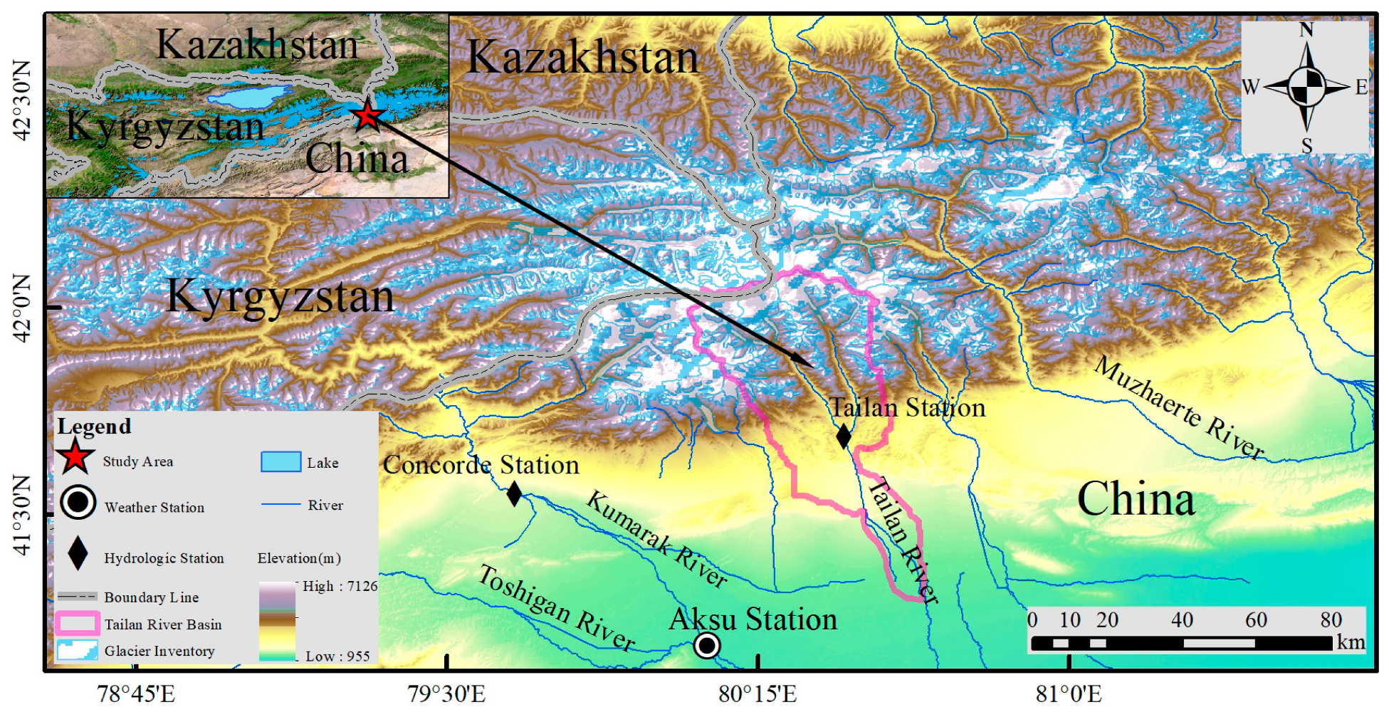
2.1. Study Area

The Tailan River basin (80°21′44″ E~81°10′44″ E, 40°41′44″ N~42°15′13″ N) is located in Aksu District, Xinjiang (Figure 1). The river originates from the southern foot of Tomur Peak in the Western Tianshan Mountains. The climate of the Tailan basin is classified as a continental arid climate, with an annual precipitation of 62 mm and evaporation of 1840 mm. The Tailan River is primarily sourced by snowmelt water at the upper reaches of the Tarim River [46]. The overall topography is characterized by high north and low south, and high west and low east. There are 115 glaciers developed in the Tailan River basin, with a total glacier area of about 431 km² and a glacier coverage rate of 32.41% in the basin. Among all the glaciers, there are 4 glaciers over 10 km², and the largest glacier is Qiongtailan Glacier, with an area of 140.93 km². The elevation changes at the end of the glaciers are mainly distributed at 3600–3900 m and 3900–4200 m.

2.2. Datasets

Sentinel-1A satellite was launched on 3 April 2014. It is the first satellite developed by the European Commission and the European Space Agency for the Copernicus Global Earth Observation Project [47]. It is mainly used for marine environmental monitoring, Arctic sea ice monitoring, and surface deformation monitoring. It has four working modes, SM, IW, EW, and WV [48]. The spatial resolution of the satellite data is 5 m × 20 m [49], the temporal resolution is 12 days, and the period can be shortened to 6 days with the co-operation of the double star. It provides a rich and effective data source for monitoring glacier elevation [50]. This paper uses Sentinel-1A data from 12 February and 24 February 2022, to obtain InSAR DEM.

The NASA DEM was modified by the SRTM (Shuttle Radar Topography Mission) for processing, elevation controlling, gap filling, and merging with data from the original SRTM production to improve elevation accuracy and fill in missing elevation data [51]. The SRTM dataset is composed of two band DEMs, C-band (5.6 GHz) and X-band (9.7 GHz), with widths of 225 km and 50 km, respectively [52]. In this paper, C-band NASA DEM (resolution is 30 m) is used as the 2000 elevation reference DEM. Due to the reduced strip width and large data gaps in the X-band SRTM [53], only the X-band DEM (resolution is 30 m) is used in this paper as the base data for GSE change error correction.

ALOS-PALSAR DEM has been used in the field of terrain analysis because of its high resolution, visualization of fine terrain, and low influence on surface cover [25]. It is currently the highest resolution and most widely distributed free DEM [54]. PALSAR has several observation modes, including FBS, FBD, and PLR [55]. In this paper, ALOS DEM (resolution is 12.5 m) is chosen as the reference DEM in 2009.

Due to the complex topography and high altitude of the Tailan River, remote-sensing meteorological data have become the main source for obtaining climate data in this area. ERA5 (ECMWF Reanalysis v5) is published by the ECMWF (European Centre for Medium-Range Weather Forecasts) [56]. Its dataset has been recorded since 1981 and provides an accurate description of past climate [57], which can be used to study glacier change with climate response.

GLDAS (Global Land Data Assimilation System) is a land surface model that provides 30 meteorological parameters including precipitation, temperature, soil moisture, and solar radiation [58]. It uses satellite data and ground-based observations to infer global land surface hydrological processes with a spatial resolution of 0.25°. Due to the complex geographical location of the Tailan River basin, obtaining measured data is challenging. Therefore, this study utilizes GLDAS runoff data from 2000 to 2022 as an adjunct to investigate glacier runoff change patterns.

The RGI 6.0 (Randolph Glacier Inventory 6.0) database, released in July 2017, was used in this paper for glacier profile confirmation and assisted estimation of glacier area in the study area [59].

Glacier thickness dataset version 3.1.0 was international standardized glacier thickness dataset. It was distributed by the World Glacier Monitoring Service on 6 October 2019, and collected from raw and remotely sensed observations by NASA’s Operation IceBridge [60]. This paper uses the glacier thickness dataset in the study area for the removal of elevation change abnormal values.

ICESat-2/ATLAS is a new generation of laser altimetry satellite launched by NASA after ICESat/GLAS. The laser footprint of ICESat-2 has a diameter of approximately 17 m with a spacing of 0.7 m. The horizontal accuracy is better than 6.5 m, and the nominal vertical accuracy is 0.1 m [23]. ICESat-2’s mission includes precise measurements of terrain and vegetation canopy heights, achieving a surface accuracy of ±13.8 m. Data collection is concentrated during the autumn and winter seasons when vegetation interference is minimal, ensuring the reliability of the data. In this study, point data from September 2021 to February 2022 were acquired in the study area to validate the accuracy of the InSAR DEM.

The data details are shown in the

Table 1. The sources of data used in this study.

Data	Date	Data Sources
Sentinel-1A	February 2022	https://search.asf.alaska.edu/ (accessed on 1 August 2022)
C-band NASA DEM	February 2000	https://search.earthdata.nasa.gov/ (accessed on 1 August 2022)
X-band SRTM DEM	February 2000	https://geoservice.dlr.de/egp/ (accessed on 1 August 2022)
ALOS DEM	February 2009	https://search.asf.alaska.edu/ (accessed on 1 August 2022)
ERA5	2000 to 2022	https://cds.climate.copernicus.eu/ (accessed on 15 August 2022)
GLDAS	2000 to 2022	https://ldas.gsfc.nasa.gov/data/ (accessed on 16 August 2022)
RGI 6.0	July 2017	http://www.glims.org/RGI/ (accessed on 1 August 2022)
ICESat-2	September 2021 to February 2022	https://nsidc.org/home (accessed on 10 August 2022)

.

2.3. Methods

The article first validates the DEM generated by InSAR using ICESat-2 for accuracy and then uses ridgelines to co-register InSAR DEM, NASA DEM, and ALOS DEM, and uses differential method to obtain GSE changes in different time periods. The GSE results are optimized according to ice thickness data and the regularity of GSE change so that the optimized results can be obtained to further estimate the glacier mass balance. Finally, the influence of glacier mass balance on Tailan River runoff are discussed. The technical route is shown in Figure 2.

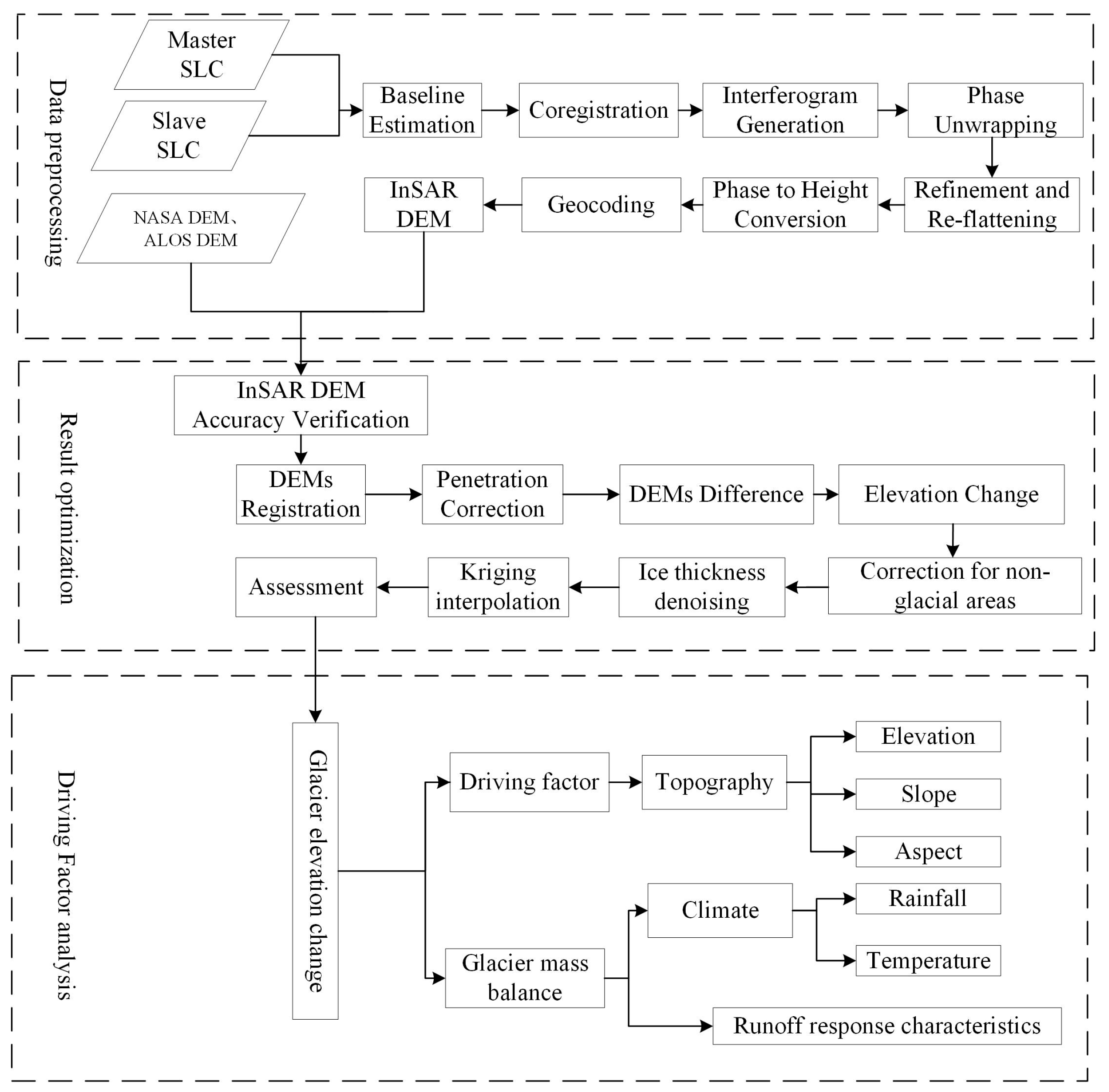
2.3.1. Production of DEM through InSAR Method

The DEM generated through Sentinel-1A includes the selection of image pairs, DEM generation, and bias correction. The selection of SAR image pairs significantly affects the accuracy of InSAR DEM generation. The optimal interferometric pairs should have a large perpendicular baseline and a small temporal baseline. Interferograms with very small perpendicular baselines (<30 m) are almost useless due to their high sensitivity to phase noise and atmospheric effects. Furthermore, the height ambiguity is inversely proportional to the spatial vertical baseline. In other words, the larger the vertical baseline, the smaller the height ambiguity, resulting in more detailed representation of surface elevation variations and dense fringes in the interferograms. Conversely, shorter spatial vertical baselines lead to larger height ambiguities and coarser representation of elevation variations. Therefore, for mapping using InSAR technology, image pairs with long spatial vertical baselines are preferred within a certain range. However, the baseline of interferometric pairs from Sentinel-1A is not very high, concentrated within the range of ±150 m, which falls short of the optimal vertical baseline achieved by ERS satellites (150–300 m) [23]. To ensure temporal consistency and proximity in data acquisition to NASA DEM and ALOS DEM, we used the ASF Baseline Tool to examine the vertical baselines of interferometric pairs during January to March 2022. Based on these criteria, we identified 7 suitable datasets, with most of the interferometric pairs having small vertical baselines (<40 m). Consequently, we selected SAR images acquired on 12 February and 24 February 2022, to generate the DEM. The vertical baseline for this interferometric pair is 60 m, well below the critical baseline of 6402 m, and associated height ambiguity is 265.690 m. The information of the SAR data is presented in the

Table 2. SAR data used in this study.

Sensor	Acquisition	Pass	Polarisation	Beam Mode
Sentinel-1A	12 February 2022	Ascending	VV	IW
Sentinel-1A	24 February 2022	Ascending	VV	IW

below.

First, the co-registration of SAR SLC (Single-Look Complex) data aims to ensure that corresponding points in the two images used for interferometric phase calculation correspond to the same point on the ground. The principle behind this process is similar to image matching in photogrammetry. In this case, SARscape 5.6.2 software was used to select the SAR image from 12 February 2022, as the master image, and the SAR image from 24 February 2022, as the slave image for registration. Registration is a crucial step in InSAR data processing as it directly affects the accuracy of the final elevation values. Two S-1 SLC split products (master and slave) of the same sub-swath are co-registered using the orbits of the two products and a DEM. The one arc-second SRTM-C DEM was employed as a vertical reference [23]. Second, the process involves conjugate multiplication of the master and slave images to obtain an interferogram. Third, to suppress speckle noise in SAR images and reduce the impact of noise in low-coherence regions, multi-looking is performed on interferograms. Given an Incidence Angle = 39.794°, PixelSpacingRg = 2.33, and PixelSpacingAz = 13.90, the ground range resolution is calculated as 9.7. The azimuth resolution is maintained at a consistent level with the ground range resolution after multi-looking, so the number of looks is set to 1 (Azimuth looks) ×5 (Range looks). As the number of looks increases, speckle noise gradually decreases, resulting in enhanced information smoothing effects. As the study area is located in a mountainous region, in order to improve the clarity of interferometric fringes and reduce decorrelation noise caused by spatial or temporal baselines, an adaptive Goldstein filter is applied for filtering. Next, to perform phase unwrapping, considering the presence of large areas of low coherence in mountainous glacial regions, the minimum-cost flow method is employed to achieve phase unwrapping. Additionally, to obtain more pixel information, the minimum coherence threshold for unwrapping is set to 0.2. Finally, terrain correction, also known as geometric correction, is the process of removing distortions and aberrations caused by the orbit, sensor, and Earth model from the raw data in radar co-ordinate system. This correction is performed using specific geometric correction methods. The corrected data are then transformed into a map projection, enabling individuals to understand and interpret the acquired geographic information more effectively. The result of the generated DEM compared with NASA DEM and ALOS DEM is shown in the Figure 3.

2.3.2. InSAR DEM Accuracy Assessment

At present, the accuracy of the DEM can be validated through various methods, primarily by comparing and evaluating it against high-precision ground control points [61], high-precision DEM models generated from airborne LiDAR point cloud data [62], and satellite-borne LiDAR height measurements [63,64], which serve as reference data. Given the complex environmental conditions and the absence of ground control point data and high-precision airborne radar data for reference in the study area, this paper employs ICESat-2 satellite altimetry data along with NASA DEM and ALOS DEM to evaluate the accuracy of the InSAR DEM. The ICESat-2 footprints were used as reference points, and data from the non-glacial region of the study area between September 2021 and February 2022 were extracted. To compare the ICESat-2 GLAS data with the DEM data, it was necessary to transform the ICESat-2 footprints and the three types of DEM data to a common plane and elevation reference. The bilinear interpolation method was applied to correspond the elevation values of ICESat-2 points to the InSAR DEM, ALOS DEM, and NASA DEM. The elevation differences were then calculated by subtracting the corresponding elevation values of ICESat-2 points, ALOS DEM, and NASA DEM from the InSAR DEM. A total of 4608 ICESat-2 points from the non-glacial region were selected as reference data. The maximum, minimum, mean, standard deviation, and root mean square error of the elevation differences with the InSAR DEM were calculated for these reference points.

2.3.3. DEM Co-Registration

Due to the limitations of imaging methods and sensors, there are differences between DEM terrains, so it is necessary to co-register DEMs. The paper proposes to correct DEMs by comparing and analyzing ridge lines. The specific method of generating ridge lines is by combining plane curvature and slope shape. The main workflow is as follows:

• Use equation $\mathrm{PNT}=\mathrm{DEM}-\mathrm{MEAN}$ to obtain the distribution areas of PNT (Positive and Negative Terrain), where “MEAN” is a 12 × 12 rectangular average value data layer obtained from DEM data through neighborhood statistics analysis;
• Extract the ridgeline by using $\mathrm{Redgeline}=\left(\mathrm{PNT}>0\right)\&(\mathrm{SOA}>80)$, where SOA (Slope of Aspect) is the planar curvature, calculated by 1 to obtain the DEM data layer “IDEM” (Inverse DEM) that is inverse to the original DEM, using the equation $\mathrm{IDEM}=\mathrm{DEM}\left(\max \right)-\mathrm{DEM}$;
• Use the ArcGIS slope tool to extract slope direction data “Aspect” from “IDEM” data, and use slope tool to extract slope “SOA2” from “Aspect” data;
• Perform the same operation as in 3 on the original DEM data to obtain “SOA1”;
• Use equation $\mathrm{SOA}=\left(\left(\mathrm{SOA}1+\mathrm{SOA}2\right)-\mathrm{abs}\left(\mathrm{SOA}1-\mathrm{SOA}2\right)\right)/2$ to obtain the planar curvature SOA.

After processing DEMs of different types, the ridge lines of three different periods (2000, 2009, and 2022) were obtained in the study area (Figure 4). Ridgeline characteristics differed across periods based on the DEM’s resolution. It is hypothesized that the elevation value along the ridge line was less affected by snow and vegetation; therefore, it is presumed that fixed points along the ridge line remain constant. Ridgeline characteristics were extracted by fitting the fixed ridge lines of the three periods. Pairwise registration was then performed to calculate the offset values of the DEM data in the x, y, and z directions based on the fitted ridge line characteristics. These values were used to shift the DEM data for repeated co-registrations, which were stopped once the offset values or standard deviation no longer decreased. After the registration is completed, the GSE change can be obtained by DEM difference calculation.

2.3.4. GSE Change Error Correction

When estimating the GMB in High Asia, the penetration of snow by the C-band had to be considered. As the DEM data used in this paper has different bands, differential estimation using the SRTM C/X band DEM in glacial areas were used to correct the penetration depth of C-band radar [65]. The elevation reference of the X-band DEM was WGS84, and, to achieve unification with the C-band DEM, EGM96 model of the Geoid height function was used to convert it to the EGM96 elevation reference. The elevation conversion steps are as follows:

• The SRTM-X band DEM raster data of the study area were converted to point features in ArcGIS 10.5 with corresponding longitude and latitude attributes added;
• Based on the point feature’s longitude and latitude co-ordinates, the Geoid height function was used to calculate the difference in elevation between the EGM96 geodetic datum and the WGS84 ellipsoid datum;
• The elevation values of the point feature were then calculated for the EGM96 elevation reference;
• The point features were converted into raster data based on the elevation reference generated on the EGM96 at a resolution of 20 m.

The average penetration depth of the C-band DEM in the Tailan River basin was found to be 2.3 ± 0.5 m. This value is processed as a systematic error when calculating GSE change. Elevation errors caused by differences in spatial resolution can be corrected by using elevation differences in non-glacier areas [65,66]. After co-registration and penetration correction, the root mean square error and standard deviation of elevation residuals between different DEM data in non-glacier areas can be preliminarily used to estimate the uncertainty of elevation change.

2.3.5. GSE Change Error Correction Based on Ice Thickness Data

The paper proposes a method of removing abnormal values by using glacier thickness data to improve the accuracy of GSE change research. The method involves extracting the glacier thickness data to the GSE change points, removing points where GSE changing values exceed the glacier thickness values, and interpolating the remaining data points.

2.3.6. GSE Change Error Correction Based on GSE Change Regularity

In order to accurately reflect the GSE changes in a given area, it is important to ensure that the map shows a smooth transition between adjacent pixels, and it also needs to conform the distribution of GSE changes; that is, elevations increase in accumulation zones and decrease in ablation zones. The Equation (1) for calculating the distribution of GMB and elevation for a specific pixel in these zones can be used to determine the elevation changes in study area [67]. Since there is no debris cover, the debris cover factor $f_{debris}$ can be treated as a constant of 1.

$$\Delta h_i=\{\begin{array}{c}\left(h_i-h_{ELA}\right)\cdot \frac{\partial \Delta h}{\partial z}{\mid }_{abl} if h_i\le h_{ELA}\\ \left(h_i-h_{ELA}\right)\cdot \frac{\partial \Delta h}{\partial z}{\mid }_{acc} if h_i>h_{ELA}\end{array}$$

(1)

Equation (1) incorporates various parameters to estimate elevation change at a given pixel. $h_{ELA}$ represents the equilibrium line altitude, while $h_i$ represents the height of the pixel $i$. The coefficients $\frac{\partial \Delta h}{\partial z}|{}_{abl}$ and $\frac{\partial \Delta h}{\partial z}|{}_{acc}$ represent slopes of GSE change relative to height in the ablation and accumulation zones, respectively. From Equation (1), it can be seen that the value of elevation changing at a certain image element can be roughly determined by determining the height position of the GMB line, and the slope of the elevation changing in the ablation and accumulation zones.

2.3.7. GSE Change and GMB Estimation

After offset correction of the DEMs, the GSE change values can be calculated. Firstly, the glacier boundary in the study area was determined based on the RGI6.0. The GSE changes from 2000 to 2009, 2009 to 2022, and 2000 to 2022 were estimated by calculating the difference between the NASA DEM, ALOS DEM, and InSAR DEM. Based on the elevation changes and glacier area, the glacier volume was calculated [68], and the GMB in the study area was estimated by using Equation (2).

$$MB=\frac{{\sum }_{i=1}^n\Delta h_i{S}_i{\rho }_{glacier}}{S_{total}{\rho }_{water}}$$

(2)

Equation (2), MB represents the GMB, $i$ denotes each altitude band, $h_i$ is the average GSE change values, $S_i$ is the glacier area corresponding to each altitude band, $S_{total}$ is the total glacier area, ${\rho }_{water}$ is the density of water, and ${\rho }_{glacier}^{}$ is the density for conversion from glacier volume to mass balance. The paper adopts the research by Huss et al. [18], wherein 850 ± 60 kg·m⁻³ is used as the glacier volume–mass conversion parameter, and ${\sigma }_{\rho }^{}$ = ±60 kg·m⁻³ is the estimated error margin for GMB calculation.

The accuracy of the DEM data, DEM co-registration and correction, and assumptions and measurement dates of glacier surface ice and snow density can all affect the precision of GMB estimation. This study uses Equation (3) to evaluate the error of the mass balance [69].

$${\sigma }_{\mathrm{geo}}=\sqrt{\Delta h^2{\sigma }_{\rho }^2+{\rho }_{glacier}^2{\sigma }_{\Delta h}^2}$$

(3)

Equation (3), ${\sigma }_{\rho }^{}$ = ±60 kg·m⁻³; $\Delta h$ represents the annual average GSE change; ${\rho }_{glacier}^{}$ is the density for conversion from glacier volume to mass balance; and ${\sigma }_{\Delta h}^{}$ is the error in GSE change, and it primarily depends on the accuracy of the DEM data. The standard deviation of elevation change in non-glacier areas can be used as an essential reference for evaluating the error in elevation change [70]. According to the theory of error propagation, the error in long-term scale elevation change is described by Equation (4).

$${\sigma }_{\Delta h}^2=\frac{{\sigma }_{\Delta h_i}^2}{N_{eff}}$$

(4)

Equation (4), ${\sigma }_{\Delta h_i}^{}$ represents the annual average elevation change of different height bands in non-glacier areas, and $N_{eff}$ represents the effective number of observed pixels.

3. Results

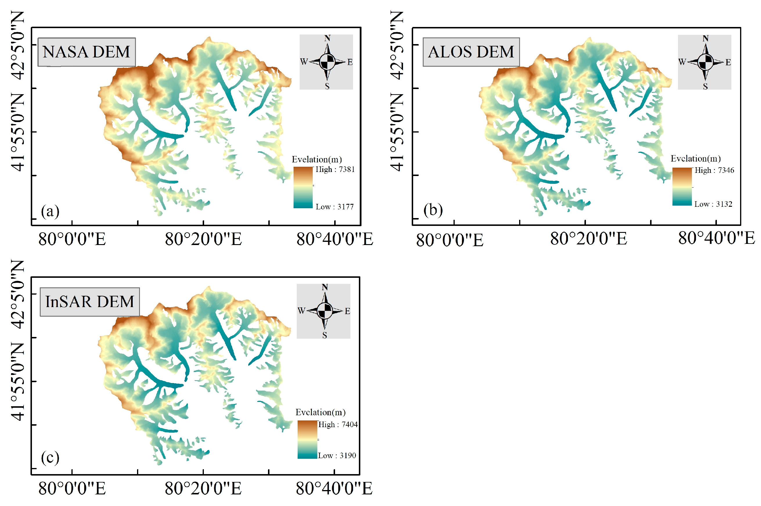
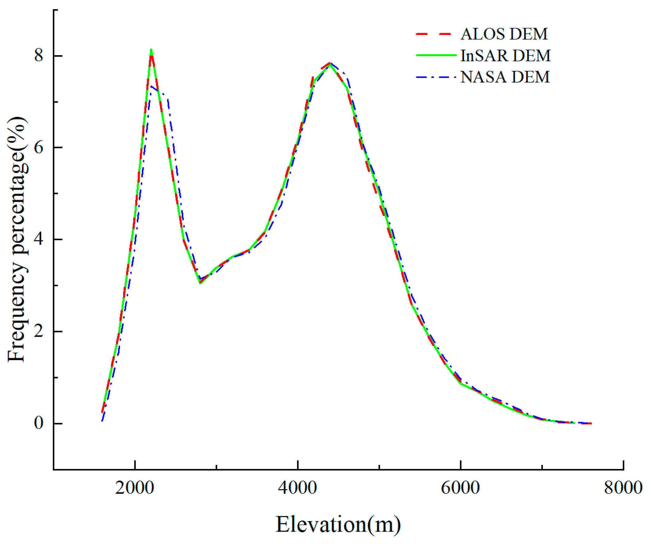
3.1. Accuracy Assessment for InSAR DEM Based on ICESat-2

Through the comparative study, the results are shown in the

Table 3. The elevation accuracy for InSAR DEM.

InSAR DEM	Min (m)	Max (m)	Mean (m)	STD (m)	RMSE (m)
ICESat-2	−31.21	23.44	−7.48	14.24	14.67
NASA DEM	−37.24	26.89	−6.62	15.45	16.42
ALOS DEM	−29.01	18.58	−4.91	10.54	9.87

; the mean elevation difference between InSAR DEM and NASA DEM (6.62 m) is smaller than the mean elevation difference between InSAR DEM and ICESat-2 (7.48 m). However, in terms of the maximum and minimum elevation differences, the latter (Min = 31.21 m, Max = 23.44 m) outperforms the former (Min = 37.24 m, Max = 26.84 m). The elevation differences between InSAR DEM and ALOS DEM are relatively small, indicating a close similarity between these two datasets. Considering the different data acquisition times, it is observed that the surface morphology changes in the non-glacial area are stable, and their magnitude is negligible compared to glacier changes. By using ridge-based DEM registration to eliminate the influence of terrain errors, the measurement accuracy of glaciers with InSAR DEM would significantly improve.

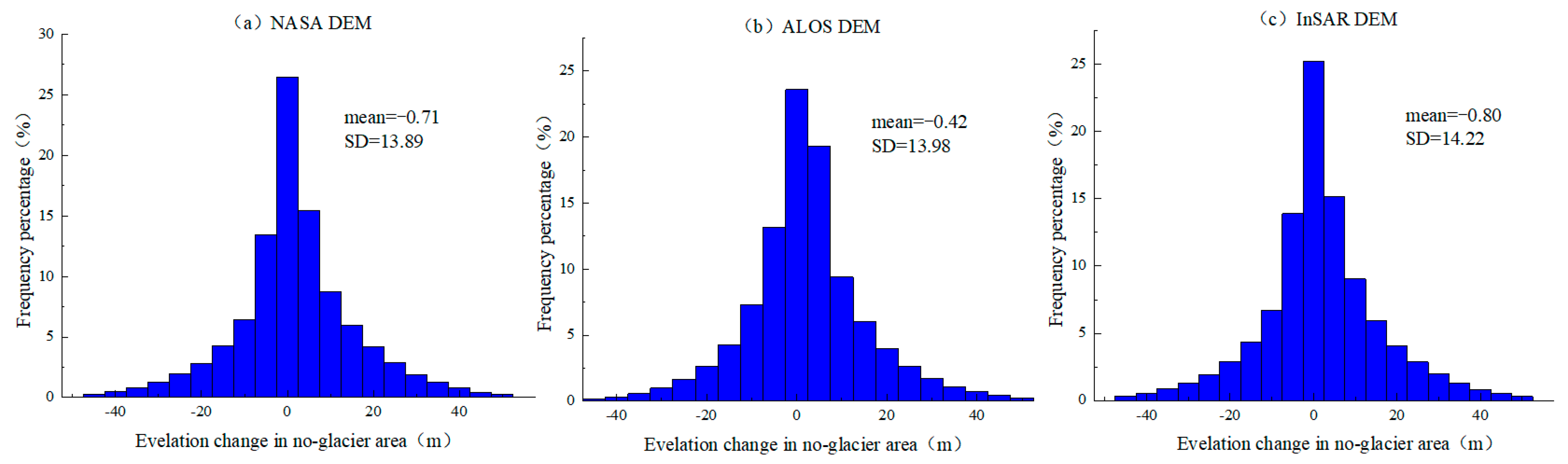
3.2. Analysis of Co-Registration and Correction Results

Table 4. The offsets in x, y, and z directions in the DEM dataset.

InSAR DEM	Offsets in x, y, and z Directions
	x (m)	y (m)	z (m)
NASA DEM	−23.9	−10.5	5.7
ALOS DEM	3.4	−6.2	−9.2

shows the offsets of co-registered DEMs in the x, y, and z directions based on ridge lines. In the x direction, the smallest offset between InSAR DEM and ALOS DEM is 3.4 m, while the largest offset between InSAR DEM and NASA DEM is 23.9 m. In the y direction, the offsets between DEMs show less variations, and most of them are concentrated in the range of 4–11 m. The smallest offset in the z direction is 5.7 m between InSAR DEM and NASA DEM. Overall, the matching error between InSAR DEM and ALOS DEM is smaller, while that between InSAR DEM and NASA DEM is larger.

Figure 5 shows the elevation distribution of the DEMs in the study area, implying that NASA DEM, ALOS DEM, and InSAR DEM data have similar elevation patterns, which suggests that these three different types of DEM data are consistent and suitable for studying GSE changes and GMB in the study area.

Differences in spatial resolution can be addressed by comparing the elevation differences in non-glacier areas. As shown in Figure 6, after co-registering and correcting the DEMs, the differences in non-glacier areas between 2000–2009, 2009–2022, and 2000–2022 are around ±20 m, with mean elevation differences of −0.71 m, −0.42 m, and −0.80 m, and deviations from the mean of 13.89, 13.98, and 14.22, respectively.

3.3. Analysis of GSE Change Optimization Results

The accuracy of the GSE changing results can be evaluated through a comparison of the standard deviation of glacier elevation changes before and after optimization. The percent change in the optimized elevation can be calculated using the equation given by (5).

$$per=\frac{{\sigma }_{Before}-{\sigma }_{Later}}{{\sigma }_{Before}}$$

(5)

The ${\sigma }_{Before}$ represents the standard deviation of the GSE change before optimization, while the ${\sigma }_{Later}$ represents the standard deviation of the GSE change after optimization.

As shown, the standard deviation of glacier elevation changing results for multiple time periods decreased by 31%, 25%, and 28% after optimization (

Table 5. Standard deviation of GSE change comparison before and after optimization.

Time	${\mathit{\sigma }}_{\mathit{B}\mathit{e}\mathit{f}\mathit{o}\mathit{r}\mathit{e}}$	${\mathit{\sigma }}_{\mathit{L}\mathit{a}\mathit{t}\mathit{e}\mathit{r}}$	per
2000–2009	10.69	7.38	31
2009–2022	10.54	7.90	25
2000–2022	15.45	11.12	28

). By using the glacier thickness data set to remove abnormal values and combining the regularity of GSE changes, the uncertainty of glacier elevation data was effectively reduced.

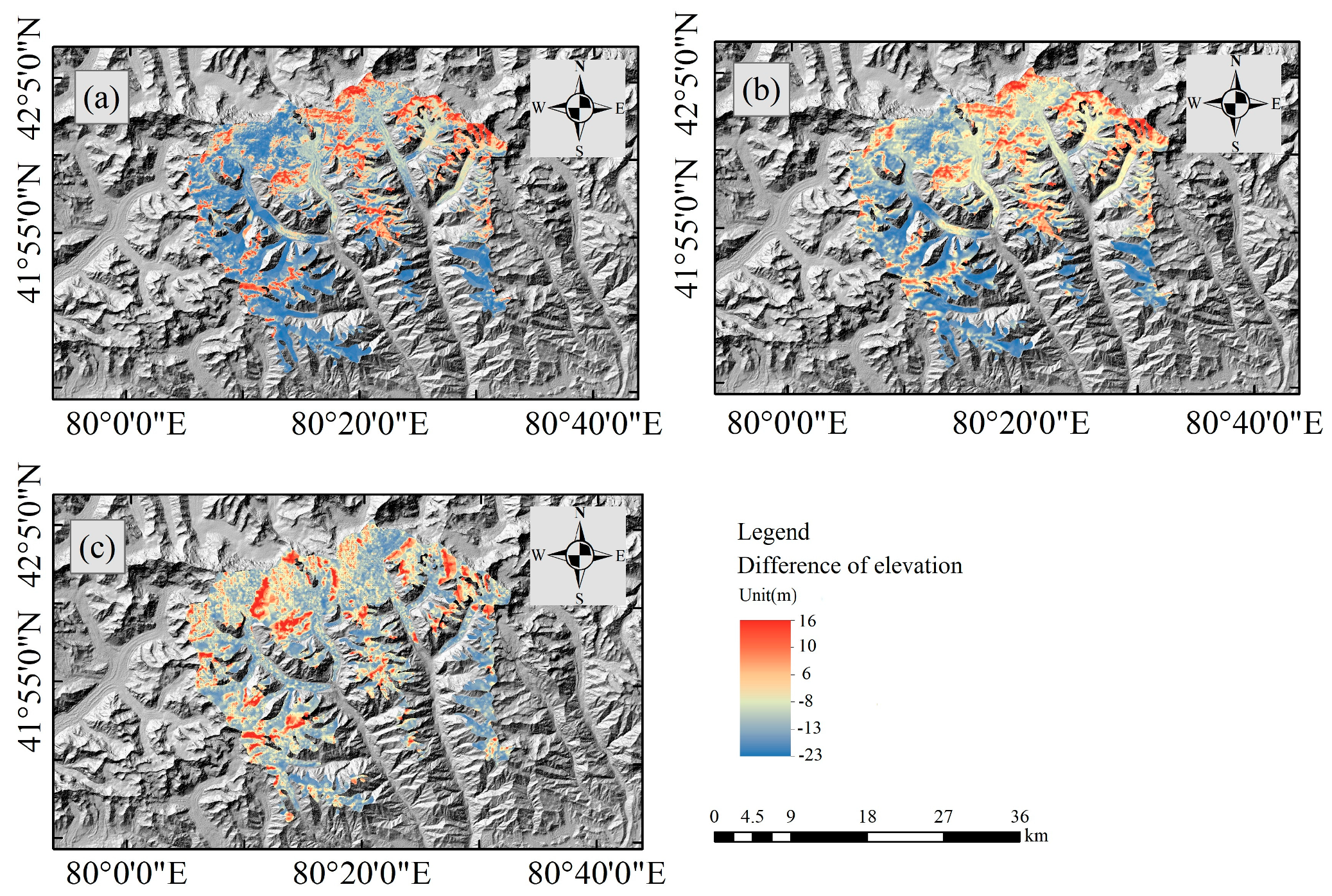
3.4. Analysis of GSE and GMB Change Results

The GSE in the Tailan River basin has shown a melting trend during different periods, with significant thinning of the majority of glacier tongues. Figure 7 shows that during the periods 2000–2009, 2009–2022, and 2000–2022, the glacier melting zones showed a significant thinning trend, while some accumulation zones showed thickening trends. The maximum thinning rate of glacier tongues was −2.4 m·a⁻¹, and the average change rate of the overall glacier elevation ranged from −2.4 m·a⁻¹ to 4.4 m·a⁻¹. In Figure 7b, the GSE decreased in some tongue zones, while high altitude zones and some tongue zones displayed thickening trends, with the maximum increase rate of the GSE reaching 1.9 m·a⁻¹. In Figure 7c, the maximum thinning rate of the GSE was −2.0 m·a⁻¹, and the average change rate of the glaciers ranged from −2.0 m·a⁻¹ to 1.3 m·a⁻¹.

The glacier zone with an altitude of 3000–5000 m was divided into altitude bands of 500 m, and the GMB at different altitudes was estimated, as shown in

Table 6. GSE change and GMB under different altitude zones.

Altitude Bands (m)	Altitude Bands Area (km2)	2000–2009		2009–2022		2000–2022
		GSE Change (m·a−1)	GMB (m w.e.a−1)	GSE Change (m·a−1)	GMB (m w.e.a−1)	GSE Change (m·a−1)	GMB (m w.e.a−1)
3000–3500	12.32	−0.43	−0.06	−0.22	−0.05	−0.13	−0.02
3500–4000	70.81	−0.30	−0.28	−0.33	−0.44	−0.31	−0.28
4000–4500	184.28	−0.32	−0.85	−0.32	−0.38	−0.24	−0.64
4500–5000	137.09	−0.21	−0.45	−0.15	−0.15	−0.21	−0.45
>5000	108.06	−0.23	−0.09	0.17	0.03	−0.38	−0.13
Total	512.56	−0.29	−0.34	−0.17	−0.19	−0.25	−0.30

, indicating the average GSE and GMB at different altitudes. The average GSE changes and GMB were negative at different altitudes (excluding the GSE change and GMB change above 5000 m altitude from 2009–2022). From 2000–2009, 2009–2022, and 2000–2022, the GSE in the study area showed a significant decline during different periods, and the glaciers had a trend of accelerating, then slowing down, and then accelerating again in their retreat. The average elevation change rates in the entire study area were −0.29 ± 0.14 m·a⁻¹, −0.17 ± 0.07 m·a⁻¹, and −0.25 ± 0.02 m·a⁻¹, respectively. Using 850 ± 60 kg·m⁻³ as the density conversion parameter, the average GMB in the Tailan River basin was calculated to be −0.34 ± 0.05 m w.e.a⁻¹, −0.19 ± 0.10 m w.e.a⁻¹, and −0.30 ± 0.02 m w.e.a⁻¹, respectively.

This paper compares and analyzes the GMB in the Tianshan area with other scholars’ research. Based on the temperature index and accumulation model, Zhang et al. [71] reconstructed the annual, summer, and winter mean mass balance of Glacier No. 51 at Hasilegen Glacier in the eastern Tianshan Mountains from 1999 to 2015. The annual, summer, and winter mean mass balance of Glacier No. 51 were −0.37 m w.e.a⁻¹, −0.54 m w.e.a⁻¹, and 0.16 ± 0.22 m w.e.a⁻¹, respectively. The results showed that temperature and annual precipitation were the main factors affecting the fluctuation of mass balance. Liu et al. [72] used multiple remote-sensing data sources, such as MOD11C3 and TRMM3B43, and established a spatial distribution degree-day model to simulate the GMB in the north and south slope basins of the Tianshan Mountains. They obtained a mass loss of −4.66 mm w.e. and an annual change rate of −0.28 mm w.e.a⁻¹ from 2000 to 2016. This study showed that glaciers in the Tianshan area have been in a negative GMB state since 2000 and confirmed the reliability of the estimated GMB in this paper.

4. Discussions

4.1. Influence of Climate on GSE Change

The temperature and precipitation data used in this paper were obtained in February, and the impact of seasonal mass balance fluctuations was ignored. Due to the lack of measured data in the Tailan River basin, it is difficult to determine the ratio of rain/snow and the conversion rate of precipitation material in this area. It is assumed that the precipitation in this area is precipitation and all of it is converted into glacial mass accumulation. As shown in Figure 8, the monthly and annual average temperatures and precipitation in the study area fluctuated significantly over time, showing a wave-like distribution. From 2000 to 2022, the average February temperature in the Tailan River basin was −15.73 °C, with the lowest temperature occurring in 2000 at −18.91 °C. The average February precipitation in the Tailan River basin from 2000–2022 was 24.76 mm. From 2000–2022, the annual average temperature and precipitation in the Tailan River basin were −6.31 °C and 287.34 mm, respectively, with the lowest annual precipitation occurring in 2022. The average February temperature and monthly precipitation from 2000–2009 fluctuated in an overall increasing trend. From 2009–2022, the annual average temperature showed a fluctuating upward trend, reaching its maximum in 2016 at −5.35 °C. The annual temperature gradually decreased after 2016 and reached a turning point in 2020, followed by an increase in temperature. From 2009–2022, precipitation showed a fluctuating downward trend, reaching a minimum of 253.78 mm in 2022.

It can be seen from the GMB changes within the basin that the greatest glacial mass loss occurred between 2000–2009, followed by 2000–2022, and the smallest mass loss occurred between 2009–2022. Compared with the 2000–2022 glacial mass loss, the 2000–2009 glacial mass loss was greater, probably because there is increased temperature and decreased precipitation from 2000 to 2009 in the study area; compared with the 2000–2022 glacier mass loss, the 2009–2022 glacier mass loss was smaller, probably because both the annual mean temperature change and the annual mean precipitation change were relatively stable from 2009 to 2022. When comparing the 2000–2009 glacial mass loss with the 2009–2022 glacial mass loss in the study area, it was clear that the 2000–2009 glacial mass loss was greater, because the annual mean precipitation had a significant decrease from 2000 to 2022, while the annual mean temperature change during this period remained stable. In other words, when the annual mean temperature change was relatively stable, the less the annual mean precipitation was, the greater the glacial mass loss was.

4.2. Influence of Topographic Factors on GSE Change

4.2.1. Influence of Altitude on GSE Change

As shown in Figure 9, glaciers in the Tailan River basin are primarily distributed on mountain peaks above an altitude of 3000 m. Over the past 22 years, almost all GSE in the basin have experienced a decrease. The overall trend indicates that the rate of decreasing GSE decreases as altitude increases. In the altitude range of 3000–4800 m, the GSE decreases sharply. It is obvious that there is a trend of the decreasing rate slowing down with altitude, and the GSE change is gradually transitioning from negative to positive in this range. This changing trend is because that zones with lower altitudes are more susceptible to temperature influences, with temperatures rising more quickly and resulting in greater glacial melting; thus, most GSEs show negative values. Above an altitude of 4800 m, the elevation of glaciers shows an increasing trend, because, that close to the ridgeline, rising altitudes and the effects of precipitation or snow accumulation can lead to glacier accumulation, so most GSE show positive values.

To validate the elevation change values obtained in this paper, a comparison was made between the glacier elevation and typical monitored glaciers elevations from other zones, as shown in

Table 7. Comparison of typical monitoring GSE.

Study Area	Time	Altitude (m)	Mean (m·a−1)	Paper
Mont Blanc	2003–2014	(1500, 4870)	0.2–0.3	[73]
Tanggula Mountain	2000–2020	(5000, 7120)	−0.76 ± 0.05	[74]
Geladandong Mountain	2012–2018 2000–2018	(4933, 6555)	−0.55 ± 0.11 −0.28 ± 0.08	[75]
Tianshan	2000–2016	(2500, 7530)	−0.28 ± 0.20	[9]
Tailan River basin	2000–2009	(944, 7392)	−0.29 ± 0.14	Research
	2009–2022		−0.17 ± 0.07
	2000–2022		−0.25 ± 0.02

. Berthier et al. [73] investigated the elevation change pattern of glaciers in the Mont Blanc area and found that the rate of glacier elevation change in the Mont Blanc range was approximately 0.2–0.3 m·a⁻¹ from 2003 to 2012. Zhou et al. [74] calculated the GSE change in the Tianshan Mountains area from 2000 to 2020 using the TanDEM-X radar data and SRTM DEM, and found that the glaciers in the eastern Tianshan Mountains had been accelerating thinning with a thinning rate of 0.76 ± 0.05 m·a⁻¹. Based on a time series of digital elevation models derived from satellite stereoscopic images, Brun F et al. [9] found that the GSE change rate in the Tianshan Mountains was −0.28± 0.20 m·a⁻¹ from 2000 to 2016. The glaciers in the Tailan River basin are located in the southern area of the West Tianshan Mountains and the conclusion drawn in this study is consistent with that of Brun F et al., which is related to the quality of the DEM, the study area, and the observation time. The reliability of the results is mainly affected by the quality of the interferometric.

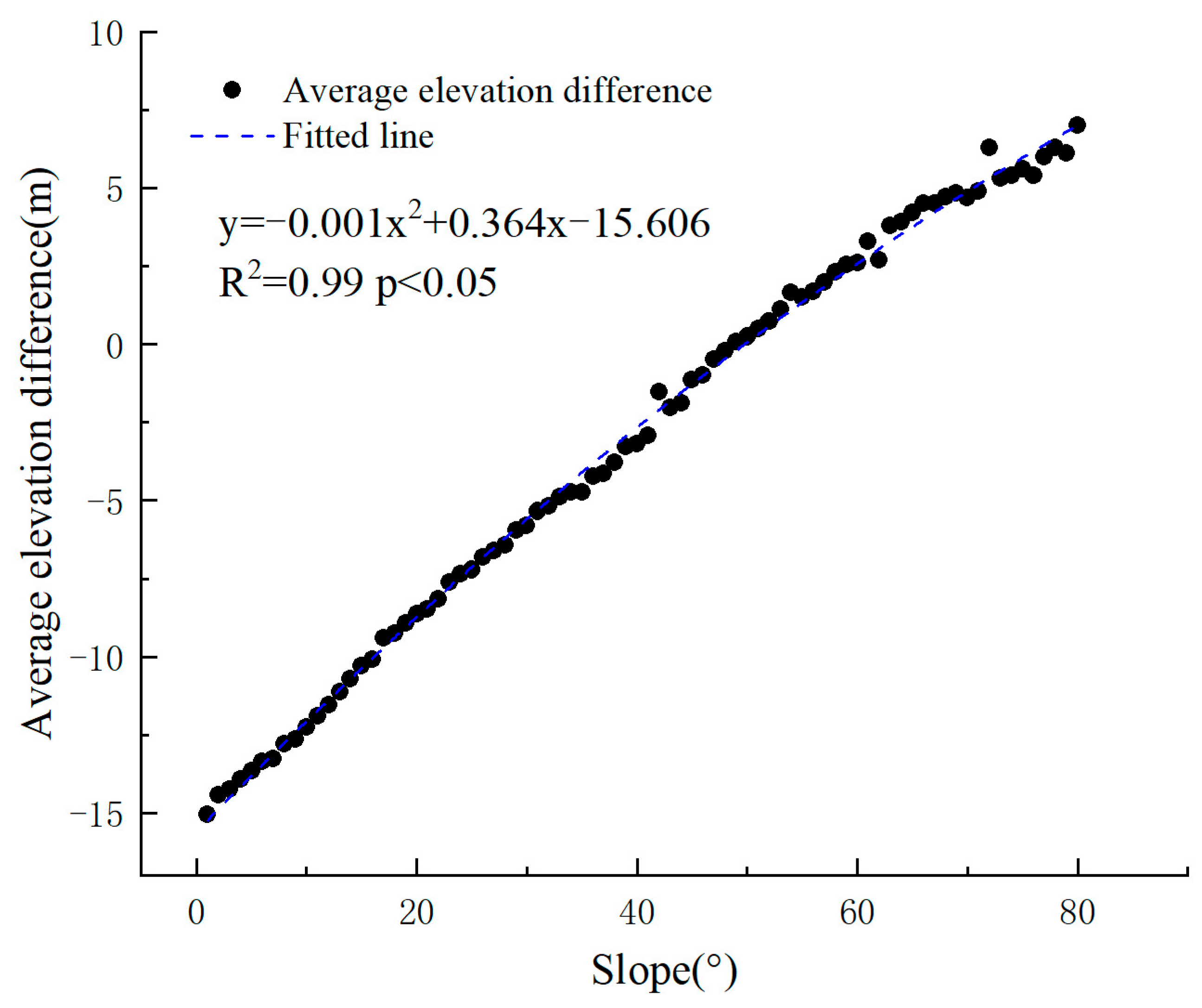
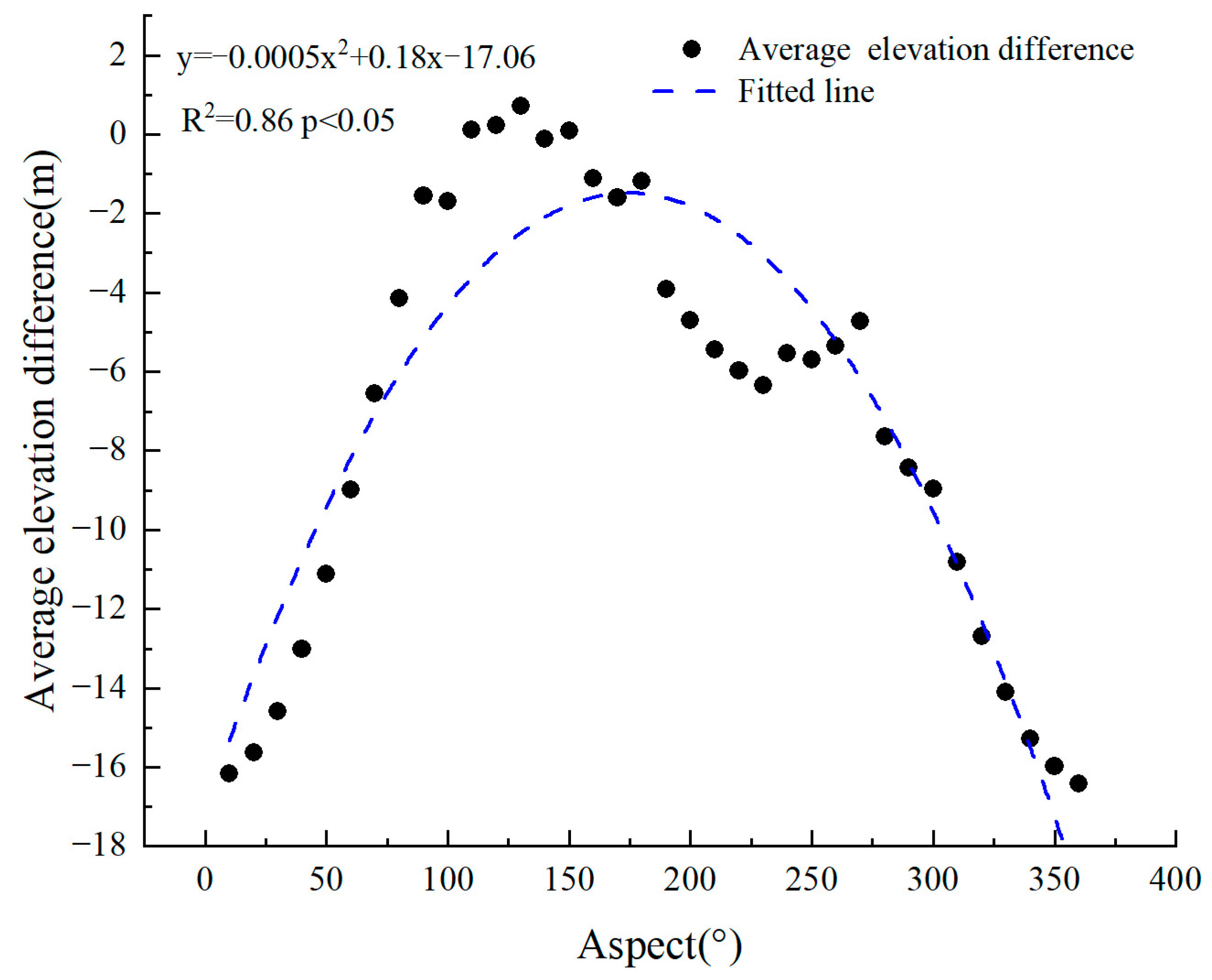
4.2.2. Influence of Slope and Aspect on GSE Change

Aspect slope was also an important factor of glacier melt [76]. To investigate the relationship between GSE change and terrain factors (slope and aspect) in the Tailan River basin, the average elevation change for glaciers was calculated for each 1° slope. Figure 10 shows a strong positive correlation (R² = 0.99) between the average GSE change and slope. The average GSE change increases with increasing slope, with negative values when the slope is less than 49° and positive values when the slope is greater than 49°. It is believed that, as the glacier slope increases and the area of receiving sunlight decreases, compared to areas with lower slopes, glaciers with a steeper slope usually have a slower melting rate. The negative value of the GSE change becomes positive, showing an accumulation phenomenon, which is consistent with the pattern of GSE and altitude change.

The average GSE change was calculated for every 10° interval. Figure 11 shows that glaciers with an aspect ranging between 0–100° and 160°–360° were thinning. To understand the distribution of glacier melt, the study area was divided into eight zones based on aspect orientation [23], with (0°–22.5°, 337.5°–360°) representing the north, (22.5°–67.5°) representing the northeast, (67.5°–112.5°) representing the east, (112.5°–157.5°) representing the southeast, (157.5°–202.5°) representing the south, (202.5°–247.5°) representing the southwest, (247.5°–292.5°) representing the west, and (292.5°–337.5°) representing the northwest. The findings revealed that glaciers facing north had the greatest thinning rate. Glaciers in the study area are located at different altitudes, and a comparison revealed that glaciers facing north are mostly situated at lower altitudes. Glaciers in the lower-altitude zones exhibit rapid melting, while those in higher-altitude zones show slow melting or even accumulation.

4.3. Influence of GMB on River Runoff

Glaciers are in a negative GMB state, and their melting has increased, increasing glacier runoff. The annual average runoff in the Tailan River Basin was 2.99 × 10⁸ m³ from 2000 to 2022, and the runoff showed a sharp decrease after 2000. Compared to 2000, the runoff decreased by 2.71 × 10⁸ m³ in 2009, with a 63% decrease. After 2009, the runoff in the Tailan River basin increased; especially from 1.56 × 10⁸ m³ in 2009 to 4.06 × 10⁸ m³ in 2010, there is an increase of 61%. Based on the conclusions in Section 3.2 of this paper, the average GMB in the Tailan River basin from 2000–2009, 2009–2022, and 2000–2022 was −0.34 ± 0.05 m w.e.a⁻¹, −0.19 ± 0.10 m w.e.a⁻¹, and −0.30 ± 0.02 m w.e.a⁻¹, respectively, with water equivalent values of 1.56 × 10⁸ m³, 6.89 × 10⁷ m³, and 1.38 × 10⁸ m³. As shown in

Table 8. Contribution rate of glacier meltwater to runoff in Tailan River basin.

Year	Mass Balance (m w.e.a−1)	Glacier Meltwater (m3)	Annual Average Runoff (m3)	Rate (%)
2000–2009	−0.34 ± 0.05	1.58 × 108	2.84 × 108	54.92
2009–2022	−0.19 ± 0.10	6.89 × 107	1.45 × 108	47.76
2000–2022	−0.30 ± 0.02	1.38 × 108	2.99 × 108	46.15

, the average annual runoff in the entire Tailan River basin from 2000–2009 was 2.84 × 10⁸ m³, with a water equivalent of 1.56 × 10⁸ m³ from glacier meltwater, accounting for 54.92% of the glacier meltwater supply. From 2009–2022, the glacier meltwater in the basin decreased by 8.71 × 10⁷ m³ compared to 2000–2009, with an average annual runoff reduction of 1.39 × 10⁸ m³.

Figure 12 shows the relationship between runoff and precipitation in the Tailan River basin. Over the past 22 years, the annual average temperature in the Tailan River basin has shown a slight upward trend, with an increasing rate of 0.08 °C·a⁻¹. In contrast, there has been a significant reduction in the total annual precipitation, with a decreasing rate of −3.2 mm·a⁻¹. During all three periods, glacier meltwater accounted for over 40% of the total runoff, with a higher contribution observed from 2000–2009 compared to 2009–2022. This trend may be related to the increasing temperature and decreasing precipitation levels. The rise in temperatures inhibits precipitation, making the snow and ice melt faster, which increases the contribution of glacier meltwater. The result found that the contribution rate of glacier melt water to runoff in the eastern and central Tianshan Mountains is between 3.5% and 67.5% [77]. It can be seen that glacier meltwater is very important for surface runoff recharge.

The paper conducted a Mann–Kendall analysis on the Tailan River basin to observe changes in runoff, and explore abrupt changes in the flow regime since 2000. As shown in Figure 13, the M–K test curve revealed that the UF curve showed a decreasing trend between 2007 and 2010, while the curve increased and surpassed the lower confidence limit of α = 0.05 in 2009–2010. The UB curve did not exceed the above limits except from 2014 to 2016. Notably, the UF and UB curves intersected at three points (2000–2002, 2010–2015, and 2020–2022), indicating abrupt changes in runoff. Nevertheless, the UF curve did not significantly exceed the confidence level during these periods. Sensitivity analysis revealed that for every 1 °C change in temperature, the GMB changed by 0.3 m, potentially causing a major annual runoff alteration of approximately 16% in the Tailan River basin.

5. Conclusions

This paper analyzes the GSE change trend and GMB state in the Tailan River basin using multiple remote-sensing data sources including glacier inventory, remote-sensing imagery, and various types of DEM data. Furthermore, this paper investigates the primary factors that affect GMB change in the study area, such as basin climate change, surface runoff, and glacier topography. The main conclusions are as follows:

• Considering the terrain differences between various types of DEMs, this paper presents a mountain ridge registration method that uses planar curvature and slope to generate mountain ridges from InSAR DEM, ALOS DEM, and NASA DEM data. The extracted mountain ridge samples are screened, fitted, and used for DEM registration based on their respective mountain ridge locations. This approach significantly improves the precision of GSE change monitoring.
• This paper proposes a glacier-thickness-data-based approach for processing glacier elevation abnormal values. The processed data result in a decrease of the standard deviation of GSE at different periods by approximately 31%, 25%, and 28%, respectively. These findings suggest that abnormal values reduction based on glacier thickness data can improve the accuracy of GSE change studies.
• This paper uses GSE change data to estimate the average annual thinning rates of glaciers for the periods 2000–2009, 2009–2022, and 2000–2022, with reduction values of−0.29 ± 0.14 m·a⁻¹, −0.17 ± 0.07 m·a⁻¹, and −0.25 ± 0.02 m·a⁻¹, respectively. The result shows that glaciers experience faster surface elevation changes in areas with lower slopes, and north-facing glaciers show higher surface thinning rates. Over the past 22 years, most glaciers in the Tailan River basin have exhibited a decline in GSE. As altitude increases, the GSE decline rate slows down, and GSE changing values shift from negative to positive.
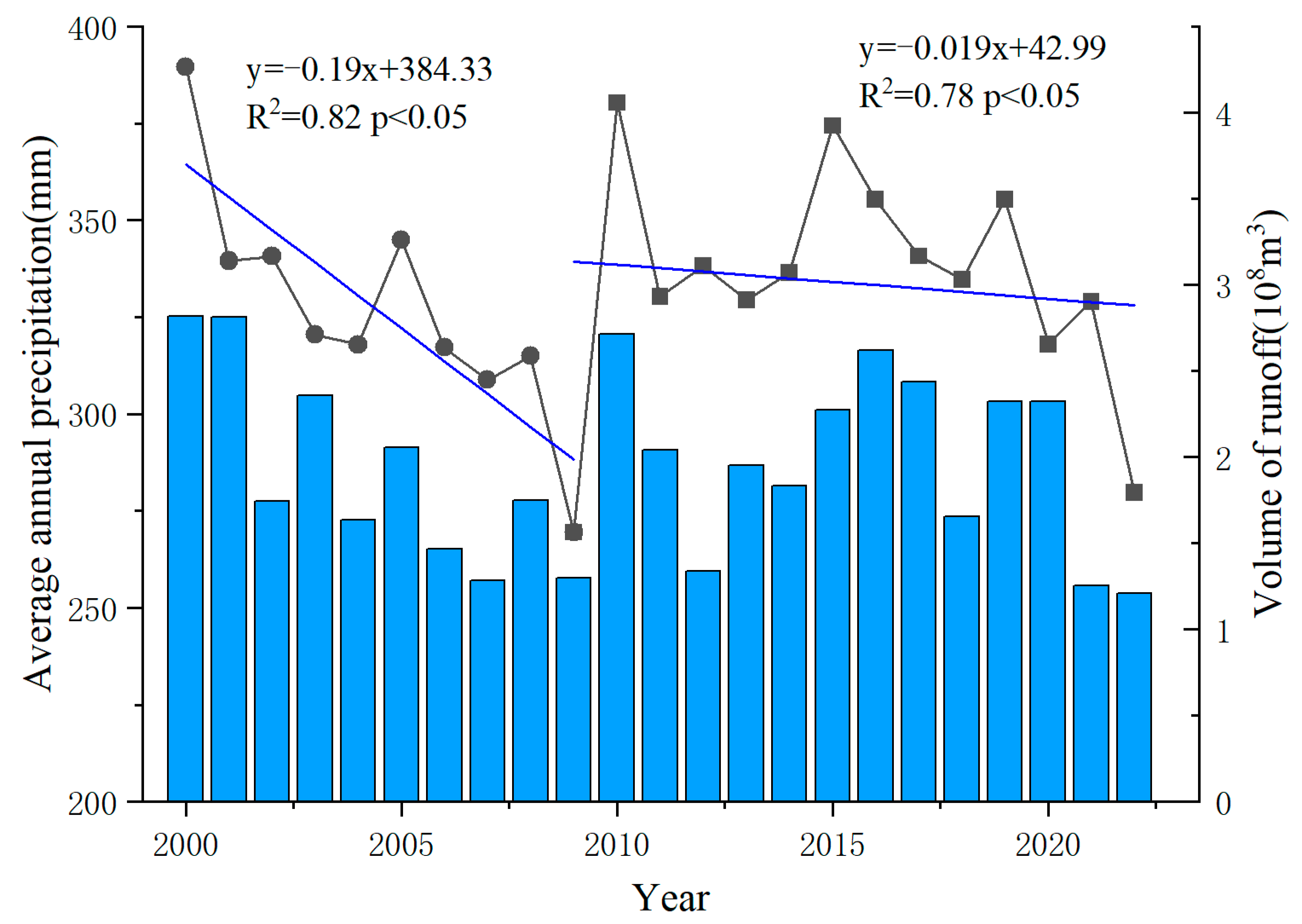
• This paper investigates the GMB changes in the study area and explored the factors that influence GMB changes, in conjunction with climate change and runoff in the basin. The results show that from 2000 to 2009, 2009 to 2022, and 2000 to 2022, the GMB change in the Tailan River basin was −0.34 ± 0.05 m w.e.a⁻¹, −0.19 ± 0.10 m w.e.a⁻¹, and −0.30 ± 0.02 m w.e.a⁻¹, respectively. The result show that the GMB in the study area was in a significant negative state. From 2000 to 2009, the average annual temperature in the Tailan River basin showed a weak upward trend with a rate of 0.08 °C·a⁻¹. The annual total precipitation exhibited a declining trend with a rate of 3.2 mm·a⁻¹. From 2000 to 2009, the change in runoff of the Tailan River basin was 2.71 × 10⁷ m³, glacial meltwater was about 6.89 × 10⁷ m³, and the largest proportion of glacial meltwater recharge was about 54.92% from 2000 to 2009. From 2009 to 2022, the runoff of the Tailan River basin was 1.45 × 10⁸ m³, and glacier meltwater accounted for approximately 47.76% of that. From 2000 to 2022, the proportion of glacier meltwater accounted for 46.15% of the runoff in the basin.

References

- Miles, E.; McCarthy, M.; Dehecq, A.; Kneib, M.; Fugger, S.; Pellicciotti, F. Health and sustainability of glaciers in High Mountain Asia. Nat. Commun. 2021, 12, 2868. [Google Scholar] [CrossRef] [PubMed]
- Bhattacharya, A.; Bolch, T.; Mukherjee, K.; King, O.; Menounos, B.; Kapitsa, V.; Neckel, N.; Yang, W.; Yao, T. High Mountain Asian glacier response to climate revealed by multi-temporal satellite observations since the 1960s. Nat. Commun. 2021, 12, 4133. [Google Scholar] [CrossRef]
- Francis, J.A.; Skific, N.; Vavrus, S.J. Increased persistence of large-scale circulation regimes over Asia in the era of amplified Arctic warming, past and future. Sci. Rep. 2020, 10, 14953. [Google Scholar] [CrossRef] [PubMed]
- Marzeion, B.; Jarosch, A.H.; Gregory, J.M. Feedbacks and mechanisms affecting the global sensitivity of glaciers to climate change. Cryosphere 2014, 8, 59–71. [Google Scholar] [CrossRef] [Green Version]
- Yao, T.; Thompson, L.; Yang, W.; Yu, W.; Gao, Y.; Guo, X.; Yang, X.; Duan, K.; Zhao, H.; Xu, B.; et al. Different glacier status with atmospheric circulations in Tibetan Plateau and surroundings. Nat. Clim. Chang. 2012, 2, 663–667. [Google Scholar] [CrossRef]
- Narama, C.; Kääb, A.; Duishonakunov, M.; Abdrakhmatov, K. Spatial variability of recent glacier area changes in the Tien Shan Mountains, Central Asia, using Corona (~1970), Landsat (~2000), and ALOS (~2007) satellite data. Glob. Planet. Chang. 2010, 71, 42–54. [Google Scholar] [CrossRef]
- Pieczonka, T.; Bolch, T.; Junfeng, W.; Shiyin, L. Heterogeneous mass loss of glaciers in the Aksu-Tarim Catchment (Central Tien Shan) revealed by 1976 KH-9 Hexagon and 2009 SPOT-5 stereo imagery. Remote Sens. Environ. 2013, 130, 233–244. [Google Scholar] [CrossRef] [Green Version]
- Shangguan, D.; Liu, S.; Ding, Y.; Ding, L.; Xiong, L.; Cai, D.; Li, G.; Lu, A.; Zhang, S.; Zhang, Y. Monitoring the glacier changes in the Muztag Ata and Konggur mountains, east Pamirs, based on Chinese Glacier Inventory and recent satellite imagery. Ann. Glaciol. 2006, 43, 79–85. [Google Scholar] [CrossRef] [Green Version]
- Brun, F.; Berthier, E.; Wagnon, P.; Kääb, A.; Treichler, D. A spatially resolved estimate of High Mountain Asia glacier mass balances from 2000 to 2016. Nat. Geosci. 2017, 10, 668–673. [Google Scholar] [CrossRef] [Green Version]
- Gardelle, J.; Berthier, E.; Arnaud, Y.; Kääb, A. Region-wide glacier mass balances over the Pamir-Karakoram-Himalaya during 1999–2011. Cryosphere 2013, 7, 1263–1286. [Google Scholar] [CrossRef] [Green Version]
- Gardner, A.S.; Moholdt, G.; Cogley, J.G.; Wouters, B.; Arendt, A.A.; Wahr, J.; Berthier, E.; Hock, R.; Pfeffer, W.T.; Kaser, G.; et al. A Reconciled Estimate of Glacier Contributions to Sea Level Rise: 2003 to 2009. Science 2013, 340, 852–857. [Google Scholar] [CrossRef] [PubMed] [Green Version]
- Sherpa, S.F.; Wagnon, P.; Brun, F.; Berthier, E.; Vincent, C.; Lejeune, Y.; Arnaud, Y.; Kayastha, R.B.; Sinisalo, A. Contrasted surface mass balances of debris-free glaciers observed between the southern and the inner parts of the Everest region (2007–15). J. Glaciol. 2017, 63, 637–651. [Google Scholar] [CrossRef] [Green Version]
- Immerzeel, W.W.; Lutz, A.F.; Andrade, M.; Bahl, A.; Biemans, H.; Bolch, T.; Hyde, S.; Brumby, S.; Davies, B.J.; Elmore, A.C.; et al. Importance and vulnerability of the world’s water towers. Nature 2020, 577, 364–369. [Google Scholar] [CrossRef]
- Zhou, Y.; Li, Z.; Li, J.; Zhao, R.; Ding, X. Glacier mass balance in the Qinghai–Tibet Plateau and its surroundings from the mid-1970s to 2000 based on Hexagon KH-9 and SRTM DEMs. Remote Sens. Environ. 2018, 210, 96–112. [Google Scholar] [CrossRef]
- Bolch, T.; Yao, T.; Kang, S.; Buchroithner, M.F.; Scherer, D.; Maussion, F.; Huintjes, E.; Schneider, C. A glacier inventory for the western Nyainqentanglha Range and the Nam Co Basin, Tibet, and glacier changes 1976–2009. Cryosphere 2010, 4, 419–433. [Google Scholar] [CrossRef] [Green Version]
- Scherler, D.; Bookhagen, B.; Strecker, M.R. Spatially variable response of Himalayan glaciers to climate change affected by debris cover. Nat. Geosci. 2011, 4, 156–159. [Google Scholar] [CrossRef]
- Huss, M. Density assumptions for converting geodetic glacier volume change to mass change. Cryosphere 2013, 7, 877–887. [Google Scholar] [CrossRef] [Green Version]
- Mayr, E.; Hagg, W. Debris-Covered Glaciers. In Geomorphology of Proglacial Systems: Landform and Sediment Dynamics in Recently Deglaciated Alpine Landscapes; Heckmann, T., Morche, D., Eds.; Springer International Publishing: Cham, Switzerland, 2019; pp. 59–71. [Google Scholar]
- Thibert, E.; Blanc, R.; Vincent, C.; Eckert, N. Glaciological and volumetric mass-balance measurements: Error analysis over 51 years for Glacier de Sarennes, French Alps. J. Glaciol. 2008, 54, 522–532. [Google Scholar] [CrossRef] [Green Version]
- Du, W.; Zheng, Y.; Li, Y.; Bao, A.; Li, J.; Ma, D.; Gao, X.; Pan, Y.; Wang, S. Recent Seasonal Spatiotemporal Variations in Alpine Glacier Surface Elevation in the Pamir. Remote Sens. 2022, 14, 4923. [Google Scholar] [CrossRef]
- Wang, P.; Xing, C.; Pan, X. Reservoir Dam Surface Deformation Monitoring by Differential GB-InSAR Based on Image Subsets. Sensors 2020, 20, 396. [Google Scholar] [CrossRef] [Green Version]
- Yan, L.; Wang, J.; Shao, D. Glacier Mass Balance in the Manas River Using Ascending and Descending Pass of Sentinel 1A/1B Data and SRTM DEM. Remote Sens. 2022, 14, 1506. [Google Scholar] [CrossRef]
- Khasanov, K.; Masharif, B. Vertical Accuracy of Freely Available Global Digital Elevation Models: A Case Study in Karaman Water Reservoir Territory. Int. J. Geoinformatics 2022, 18, 53–61. [Google Scholar]
- Sadhasivam, N.; Periasamy, T.; Rahaman, S.A.; Rajagopal, J. Erosion risk assessment through morphometric indices for prioritisation of Arjuna watershed using ALOS-PALSAR DEM. Model. Earth Syst. Environ. 2019, 5, 907–924. [Google Scholar] [CrossRef]
- Uuemaa, E.; Ahi, S.; Montibeller, B.; Muru, M.; Kmoch, A. Vertical Accuracy of Freely Available Global Digital Elevation Models (ASTER, AW3D30, MERIT, TanDEM-X, SRTM, and NASADEM). Remote Sens. 2020, 12, 3482. [Google Scholar] [CrossRef]
- Tachikawa, T.; Kaku, M.; Iwasaki, A.; Gesch, D.; Oimoen, M.; Zhang, Z.; Danielson, J.; Krieger, T.; Curtis, B.; Haase, J. ASTER Global Digital Elevation Model Version 2—Summary of Validation Results; NASA: Washington, DC, USA, 2011. [Google Scholar]
- Kyriou, A.; Nikolakopoulos, K. Assessing the suitability of Sentinel-1 data for landslide mapping. Eur. J. Remote Sens. 2018, 51, 402–411. [Google Scholar] [CrossRef] [Green Version]
- Mäkynen, M.; Karvonen, J. Incidence Angle Dependence of First-Year Sea Ice Backscattering Coefficient in Sentinel-1 SAR Imagery Over the Kara Sea. IEEE Trans. Geosci. Remote Sens. 2017, 55, 6170–6181. [Google Scholar] [CrossRef]
- Mu, C.; Peng, X.; Du, R.; Liu, H.; Jin, H.; Liang, B.; Mu, M.; Sun, W.; Fan, C.; Wu, X.; et al. A Comprehensive Dataset for Earth System Models in a Permafrost Region: Meteorological, Permafrost, and Carbon Observations (2011–2020) in Northeastern Qinghai-Tibet Plateau. Earth Syst. Sci. Data Discuss. 2022, 2022, 1–32. [Google Scholar] [CrossRef]
- Xu, S.; Wang, Y.; Wang, Y.; Qi, S.; Zhou, M. Glacier Mass Balance Changes Over the Turgen Daban Range, Western Qilian Shan, From 1966/75 to 2020. Front. Earth Sci. 2022, 10, 848895. [Google Scholar] [CrossRef]
- Gao, X.; Ye, B.; Zhang, S.; Qiao, C.; Zhang, X. Glacier runoff variation and its influence on river runoff during 1961–2006 in the Tarim River Basin, China. Sci. China Earth Sci. 2010, 53, 880–891. [Google Scholar] [CrossRef]
- Braithwaite, R.J.; Zhang, Y. Sensitivity of mass balance of five Swiss glaciers to temperature changes assessed by tuning a degree-day model. J. Glaciol. 2000, 46, 7–14. [Google Scholar] [CrossRef] [Green Version]
- Pope, A. GLOSSARY OF GLACIER MASS BALANCE AND RELATED TERMS. J.G. Cogley, R. Hock, L.A. Rasmussen, A.A. Arendt, A. Bauder, R.J. Braithwaite, P. Jansson, G. Kaser, M. Möller, L. Nicholson, and M. Zemp. 2011. Paris: UNESCO-IHP (IHP-VII Technical documents in hydrology 86, IACS contribution 2), vi + 114p, illustrated, soft cover. Polar Rec. 2012, 48, e15. [Google Scholar] [CrossRef] [Green Version]
- Ahluwalia, R.S.; Rai, S.P.; Meetei, P.N.; Kumar, S.; Sarangi, S.; Chauhan, P.; Karakoti, I. Spatial-diurnal variability of snow/glacier melt runoff in glacier regime river valley: Central Himalaya, India. Quat. Int. 2021, 585, 183–194. [Google Scholar] [CrossRef]
- Radić, V.; Hock, R. Glaciers in the Earth’s Hydrological Cycle: Assessments of Glacier Mass and Runoff Changes on Global and Regional Scales. Surv. Geophys. 2014, 35, 813–837. [Google Scholar] [CrossRef]
- Van Pelt, W.J.J.; Pohjola, V.A.; Pettersson, R.; Ehwald, L.E.; Reijmer, C.H.; Boot, W.; Jakobs, C.L. Dynamic Response of a High Arctic Glacier to Melt and Runoff Variations. Geophys. Res. Lett. 2018, 45, 4917–4926. [Google Scholar] [CrossRef] [Green Version]
- Lutz, A.F.; Immerzeel, W.W.; Shrestha, A.B.; Bierkens, M.F.P. Consistent increase in High Asia’s runoff due to increasing glacier melt and precipitation. Nat. Clim. Change 2014, 4, 587–592. [Google Scholar] [CrossRef] [Green Version]
- Ma, N.; Zhang, Y. Increasing Tibetan Plateau terrestrial evapotranspiration primarily driven by precipitation. Agric. For. Meteorol. 2022, 317, 108887. [Google Scholar] [CrossRef]
- Zhao, J.; Wang, J.; Harbor, J.M.; Liu, S.; Yin, X.; Wu, Y. Quaternary glaciations and glacial landform evolution in the Tailan River valley, Tianshan Range, China. Quat. Int. 2015, 358, 2–11. [Google Scholar] [CrossRef]
- Yongping, S.; Zichu, X.; Liangfu, D.; Jingshi, L. Estimation of Average Mass Balance for Glaciers in a Water Shed and Its Application. J. Glaciol. Geocryol. 1997, 19, 302–307. [Google Scholar]
- Shen, Y.P.; Liu, S.Y.; Ding, Y.J.; Wang, S. Glacier Mass Balance Change in Tailanhe River Watersheds on the South Slope of the Tianshan Mountains and Its Impact on Water Resources. J. Glaciol. Geocryol. 2003, 25, 124–129. [Google Scholar] [CrossRef]
- Liu, S.; Ding, Y.; Zhang, Y.; Shangguan, D.; Li, J.; Han, H.; Wang, J.; Xie, C. Impact of the glacial change on water resources in the Tarim River Basin. Acta Geogr. Sin. 2006, 61, 482–490. [Google Scholar]
- Zhao, G.; Zhang, Z.; Liu, L.; Li, Z.; Wang, P.; Xu, L. Simulation and construction of the glacier mass balance in the Manas River Basin, Tianshan, China from 2000 to 2016. J. Geogr. Sci. 2020, 30, 988–1004. [Google Scholar] [CrossRef]
- Wu, P.; Shu, L.; Yang, C.; Xu, Y.; Zhang, Y. Simulation of groundwater flow paths under managed abstraction and recharge in an analogous sand-tank phreatic aquifer. Hydrogeol. J. 2019, 27, 3025–3042. [Google Scholar] [CrossRef]
- Chang, L.; Chen, Y.-T.; Wang, J.-H.; Chang, Y.-L. Rice-Field Mapping with Sentinel-1A SAR Time-Series Data. Remote Sens. 2021, 13, 103. [Google Scholar] [CrossRef]
- Aðalgeirsdóttir, G.; Magnússon, E.; Pálsson, F.; Thorsteinsson, T.; Belart, J.M.C.; Jóhannesson, T.; Hannesdóttir, H.; Sigurðsson, O.; Gunnarsson, A.; Einarsson, B.; et al. Glacier Changes in Iceland From ~1890 to 2019. Front. Earth Sci. 2020, 8, 523646. [Google Scholar] [CrossRef]
- Zhang, T.; Shen, W.-B.; Wu, W.; Zhang, B.; Pan, Y. Recent Surface Deformation in the Tianjin Area Revealed by Sentinel-1A Data. Remote Sens. 2019, 11, 130. [Google Scholar] [CrossRef] [Green Version]
- Yague-Martinez, N.; Prats-Iraola, P.; Gonzalez, F.; Brcic, R.; Shau, R.; Geudtner, D.; Eineder, M.; Bamler, R. Interferometric Processing of Sentinel-1 TOPS Data. IEEE Trans. Geosci. Remote Sens. 2016, 54, 2220–2234. [Google Scholar] [CrossRef] [Green Version]
- Zhou, M.; Xu, S.; Wang, Y.; Wang, Y.; Hou, S. Recent 50-Year Glacier Mass Balance Changes over the Yellow River Source Region, Determined by Remote Sensing. Remote Sens. 2022, 14, 6286. [Google Scholar] [CrossRef]
- Paul, F.; Bolch, T.; Kääb, A.; Nagler, T.; Nuth, C.; Scharrer, K.; Shepherd, A.; Strozzi, T.; Ticconi, F.; Bhambri, R.; et al. The glaciers climate change initiative: Methods for creating glacier area, elevation change and velocity products. Remote Sens. Environ. 2015, 162, 408–426. [Google Scholar] [CrossRef] [Green Version]
- Chen, F.; Wang, J.; Li, B.; Yang, A.; Zhang, M. Spatial variability in melting on Himalayan debris-covered glaciers from 2000 to 2013. Remote Sens. Environ. 2023, 291, 113560. [Google Scholar] [CrossRef]
- Du, W.; Liu, X.; Guo, J.; Shen, Y.; Li, W.; Chang, X. Analysis of the melting glaciers in Southeast Tibet by ALOS-PALSAR data. Terr. Atmos. Ocean. Sci. 2019, 30, 7–19. [Google Scholar] [CrossRef] [Green Version]
- Wang, L.; Marzahn, P.; Bernier, M.; Jacome, A.; Poulin, J.; Ludwig, R. Comparison of TerraSAR-X and ALOS PALSAR Differential Interferometry with Multisource DEMs for Monitoring Ground Displacement in a Discontinuous Permafrost Region. IEEE J. Sel. Top. Appl. Earth Obs. Remote Sens. 2017, 10, 4074–4093. [Google Scholar] [CrossRef]
- Yilmaz, M. Accuracy assessment of temperature trends from ERA5 and ERA5-Land. Sci. Total Environ. 2023, 856, 159182. [Google Scholar] [CrossRef] [PubMed]
- Hussain, M.A.; Azam, M.F.; Srivastava, S.; Vinze, P. Positive mass budgets of high-altitude and debris-covered fragmented tributary glaciers in Gangotri Glacier System, Himalaya. Front. Earth Sci. 2022, 10, 978836. [Google Scholar] [CrossRef]
- Ramirez, S.G.; Hales, R.C.; Williams, G.P.; Jones, N.L. Extending SC-PDSI-PM with neural network regression using GLDAS data and Permutation Feature Importance. Environ. Model. Softw. 2022, 157, 105475. [Google Scholar] [CrossRef]
- Muhammad, S.; Tian, L.; Khan, A. Early twenty-first century glacier mass losses in the Indus Basin constrained by density assumptions. J. Hydrol. 2019, 574, 467–475. [Google Scholar] [CrossRef]
- Welty, E.; Zemp, M.; Navarro, F.; Huss, M.; Fürst, J.; Gärtner-Roer, I.; Landmann, J.; Machguth, H.; Naegeli, K.; Andreassen, L.M.; et al. Worldwide version-controlled database of glacier thickness observations. Earth Syst. Sci. Data 2020, 12, 3039–3055. [Google Scholar] [CrossRef]
- Rehman, K.; Fareed, N.; Chu, H.-J. NASA ICESat-2: Space-Borne LiDAR for Geological Education and Field Mapping of Aeolian Sand Dune Environments. Remote Sens. 2023, 15, 2882. [Google Scholar] [CrossRef]
- Ferretti, A.; Monti-Guarnieri, A.; Prati, C.; Rocca, F.; Massonet, D. InSAR Principles—Guidelines for SAR Interferometry Processing and Interpretation; ESA Publication: Noordwijk, The Netherlands, 2007. [Google Scholar]
- Malik, K.; Kumar, D. High Resolution Interferometric Digital Elevation Model Generation and Validation. Int. Arch. Photogramm. Remote Sens. Spat. Inf. Sci. 2018, 42, 755–756. [Google Scholar] [CrossRef] [Green Version]
- Tang, X.; Zhou, P.; Zhang, G.; Wang, X.; Jiang, Y.; Guo, L.; Liu, S. Verification of ZY-3 Satellite Imagery Geometric Accuracy Without Ground Control Points. IEEE Geosci. Remote Sens. Lett. 2015, 12, 2100–2104. [Google Scholar] [CrossRef]
- Yue, L.; Shen, H.; Zhang, L.; Zheng, X.; Zhang, F.; Yuan, Q. High-quality seamless DEM generation blending SRTM-1, ASTER GDEM v2 and ICESat/GLAS observations. ISPRS J. Photogramm. Remote Sens. 2017, 123, 20–34. [Google Scholar] [CrossRef]
- Li, Y.; Fu, H.; Zhu, J.; Wu, K.; Yang, P.; Wang, L.; Gao, S. A Method for SRTM DEM Elevation Error Correction in Forested Areas Using ICESat-2 Data and Vegetation Classification Data. Remote Sens. 2022, 14, 3380. [Google Scholar] [CrossRef]
- Gardelle, J.; Berthier, E.; Arnaud, Y. Impact of resolution and radar penetration on glacier elevation changes computed from DEM differencing. J. Glaciol. 2012, 58, 419–422. [Google Scholar] [CrossRef] [Green Version]
- Paul, F. Calculation of glacier elevation changes with SRTM: Is there an elevation-dependent bias? J. Glaciol. 2008, 54, 945–946. [Google Scholar] [CrossRef] [Green Version]
- Farinotti, D.; Huss, M.; Bauder, A.; Funk, M.; Truffer, M. A method to estimate the ice volume and ice-thickness distribution of alpine glaciers. J. Glaciol. 2009, 55, 422–430. [Google Scholar] [CrossRef] [Green Version]
- Denzinger, F.; Machguth, H.; Barandun, M.; Berthier, E.; Girod, L.; Kronenberg, M.; Usubaliev, R.; Hoelzle, M. Geodetic mass balance of Abramov Glacier from 1975 to 2015. J. Glaciol. 2021, 67, 331–342. [Google Scholar] [CrossRef]
- Huss, M.; Bauder, A.; Funk, M. Homogenization of long-term mass-balance time series. Ann. Glaciol. 2009, 50, 198–206. [Google Scholar] [CrossRef] [Green Version]
- Bolch, T.; Pieczonka, T.; Mukherjee, K.; Shea, J. Brief communication: Glaciers in the Hunza catchment (Karakoram) have been nearly in balance since the 1970s. Cryosphere 2017, 11, 531–539. [Google Scholar] [CrossRef] [Green Version]
- Zhang, H.; Li, Z.Q.; Zhou, P.; Zhu, X.F.; Wang, L. Mass-balance observations and reconstruction for Haxilegen Glacier No. 51, eastern Tien Shan, from 1999 to 2015. J. Glaciol. 2018, 64, 689–699. [Google Scholar] [CrossRef] [Green Version]
- Liu, L.; Tian, H.; Zhang, X.Y.; Chen, H.J.; Zhang, Z.Y.; Zhao, G.N.; Kang, Z.W.; Wang, T.X.; Gao, Y.; Yu, F.C.; et al. Analysis of Spatiotemporal Heterogeneity of Glacier Mass Balance on the Northern and Southern Slopes of the Central Tianshan Mountains, China. Water 2022, 14, 1601. [Google Scholar] [CrossRef]
- Berthier, E.; Cabot, V.; Vincent, C.; Six, D. Decadal Region-Wide and Glacier-Wide Mass Balances Derived from Multi-Temporal ASTER Satellite Digital Elevation Models. Validation over the Mont-Blanc Area. Front. Earth Sci. 2016, 4, 63. [Google Scholar] [CrossRef] [Green Version]
- Zhou, Y.; Li, X.; Zheng, D.; Zhang, X.; Wang, Y.; Ren, S.; Guo, Y. Decadal Changes in Glacier Area, Surface Elevation and Mass Balance for 2000–2020 in the Eastern Tanggula Mountains Using Optical Images and TanDEM-X Radar Data. Remote Sens. 2022, 14, 506. [Google Scholar] [CrossRef]
- Liu, L.; Jiang, L.; Zhang, Z.; Wang, H.; Ding, X. Recent Accelerating Glacier Mass Loss of the Geladandong Mountain, Inner Tibetan Plateau, Estimated from ZiYuan-3 and TanDEM-X Measurements. Remote Sens. 2020, 12, 472. [Google Scholar] [CrossRef] [Green Version]
- Abdullah, T.; Romshoo, S.A.; Rashid, I. The satellite observed glacier mass changes over the Upper Indus Basin during 2000–2012. Sci. Rep. 2020, 10, 14285. [Google Scholar] [CrossRef] [PubMed]
- Zhang, Y.; Luo, Y.; Sun, L.; Liu, S.; Chen, X.; Wang, X. Using glacier area ratio to quantify effects of melt water on runoff. J. Hydrol. 2016, 538, 269–277. [Google Scholar] [CrossRef]