Research on a Prediction Model of Water Quality Parameters in a Marine Ranch Based on LSTM-BP

Abstract

Water quality is an important factor affecting marine pasture farming. Water quality parameters have the characteristics of time series, showing instability and nonlinearity. Previous water quality prediction models are usually based on specific assumptions and model parameters, which may have limitations for complex water environment systems. Therefore, in order to solve the above problems, this paper combines long short-term memory (LSTM) and backpropagation (BP) neural networks to construct an LSTM-BP combined water quality parameter prediction model and uses the root mean square error (RMSE), mean absolute error (MAE), and Nash-Sutcliffe efficiency coefficient (NSE) to evaluate the model. Experimental results show that the prediction performance of the LSTM-BP model is better than other models. On the RMSE and MAE indicators, the LSTM-BP model is 76.69% and 79.49% lower than other models, respectively. On the NSE index, the LSTM-BP model has improved by 34.13% compared with other models. The LSTM-BP model can effectively reflect time series characteristics and nonlinear mapping capabilities. This research provides a new method and reference for the prediction of water quality parameters in marine ranching and further enables the intelligent and sustainable development of marine ranching.

1. Introduction

The ocean is a fluid entity that has huge cognitive value. A scientific understanding of the ocean is the first step to realizing the sustainable development of the ocean [1]. With the continuous improvement of observation technology, marine science has entered the era of big data, and the combination with artificial intelligence is obviously convenient [2]. Marine ranching is an important part of the fishery economy. Modern marine ranching combines traditional marine ranching with big data, artificial intelligence, and other technologies to perform multi-parameter monitoring, data collection, and data prediction on marine ranching. Predicting the ecological parameters of marine ranching can provide a theoretical reference for the optimal layout of marine ranching, provide a basis for effectively evaluating the construction effect of marine ranching, guide enterprises to formulate production and harvesting strategies, and ensure healthy and continuous operation.

At present, prediction methods based on ocean parameters can be mainly divided into the time series method and the regression prediction method. The time series method is applicable to the relevant variables of the things to be predicted represented by time. According to the historical data of the predicted things changing over time, it is possible to infer the law of their changing over time and quantitatively predict the development trend of things [3]. The regression prediction method is applicable to causal relationships between the variables of the things to be predicted, finding out certain factor variables that affect the result, establishing a mathematical model according to the causal relationship, and predicting the change in the result variable according to the change in the factor variable, so as to predict the direction of development and the law of specific numerical changes. The method includes the linear regression prediction method, the multiple linear regression prediction method, the nonlinear regression prediction method, etc. [4]. Time series analysis only focuses on one variable, focusing on the trend of a variable over time; meanwhile, regression analysis involves independent variables and dependent variables, focusing on the explanatory ability and predictive effect of the independent variable on the dependent variable.

In recent years, in order to improve the prediction accuracy of water quality parameters, different water quality prediction models have been developed. Graf et al. [5] proposed a hybrid model combining discrete wavelet transform and artificial neural networks to predict water temperature. Wen et al. [6] used a wavelet analysis-artificial neural network to predict groundwater level. Zhang et al. [7] proposed a new minimum absolute shrinkage and selection operator lasso regression model including temporal autocorrelation for prediction and mechanism research of coastal Sulfide Stress Corrosion Cracking. Gauch et al. [8] used a single long-term short-term memory network to predict rainfall and runoff on multiple time scales. Chen et al. [9] conducted uncertainty analysis on the sediment load estimation model and applied the lower bound estimation method in the couplet neural network model for the first time. The deep learning models DeepAR [10], RNN [11], and TPA-LSTM [12] adopt deep learning techniques based on a recurrent neural network (RNN), in which long-term dependencies in sequences can be captured by adaptively updating hidden layers. These models enable the network to preserve and update historical information through a time-recurrent structure to better predict data. However, these neural network-based methods also have some challenges and limitations. First, choosing an appropriate network structure is crucial to the performance of the model. Finding the optimal network structure is usually done empirically and by trial and error, which can require significant time and computational resources. Secondly, for complex time series data, data preprocessing and feature extraction are also difficult tasks. It is usually necessary to select appropriate input variables and their combinations according to specific problems in order to achieve better prediction results. Other models are based on machine learning and heuristic algorithms, such as the Bayesian hierarchical statistical model developed by Guo et al. [13] to predict river water quality. Lu et al. [14] proposed two machine learning models based on hybrid decision trees to obtain more accurate short-term water quality prediction results. Wang et al. [15] proposed a new dynamic firefly algorithm to predict water resources. Green et al. [16] used support vector machines (SVM) and random forests to predict river solute concentrations. Willard et al. [17] used meta-transfer learning to predict water temperature in unmonitored lakes. Kargar et al. [18] used Gaussian process regression (GPR), support vector regression (SVR), an M5 model tree, and random forest (RF) to estimate longitudinal dispersion coefficient (LDC) values in natural streams and rivers. Although models based on machine learning and heuristic algorithms are easy to implement, these methods have some limitations. First, these methods usually use local feature modeling, i.e., only considering recent time series data, and local feature modeling cannot capture these complex internal generative mechanisms, limiting the accuracy and stability of predictions. Second, the prediction performance is highly dependent on the choice of parameters, and different parameter choices may lead to completely different prediction results, which increases the difficulty of model selection and tuning. Finally, it is often not possible to implement a mapping function from input to output. They lack the ability to model complex nonlinear relationships in time series data.

The purpose of this study is to overcome the dependence of traditional forecasting model parameters, solve the problem of weak nonlinear mapping ability in LSTM neural network forecasting, and construct the LSTM-BP combination model. This combination can give full play to the time series modeling ability of LSTM and has strong nonlinear mapping ability so that the model can better predict time series data, thereby improving the accuracy and reliability of prediction. This model can accurately predict the key water quality parameters of the marine ranch, making the marine ranch an intelligent and sustainable development operation.

This study first introduces the collection and processing of marine pasture parameters. In the database of the marine pasture water quality monitoring system, the three parameters of chlorophyll, turbidity, and dissolved oxygen are selected for prediction experiments. Data preprocessing is performed on selected data. Then, the LSTM-BP combination model is constructed and the traditional time series forecasting method LSTM neural network is selected, along with the (Particle Swarm Optimization) PSO-BP combination model, and SVM in machine learning is used as a control experiment. Finally, the LSTM-BP network model and the experimental results of the three control experiments are analyzed and discussed.

2. Data Source and Data Processing

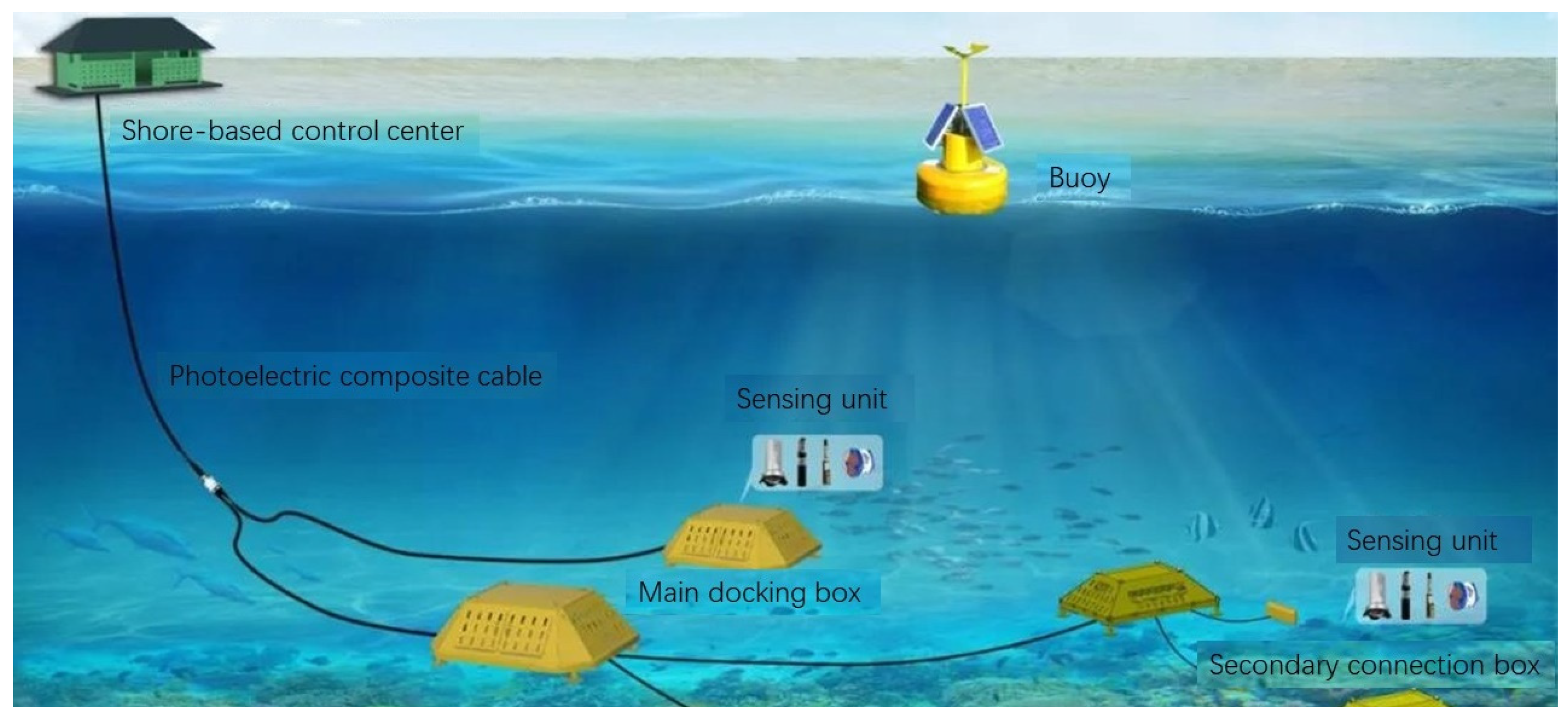
2.1. Monitoring System Structure and Data Acquisition

The data set for the experiment in this paper comes from the water quality monitoring system of Luhaifeng Marine Ranch in Qingdao City, Shandong Province, China. As shown in Figure 1, it consists of a shore station, a connection box, a data collector, a photoelectric composite cable, a water quality monitoring sensor, and an underwater camera. The function of the data collector product can integrate an optical dissolved oxygen sensor, a CTD sensor, a pH sensor, a chlorophyll turbidity sensor, and an underwater camera. The barge box and photoelectric composite cable are transmitted to the shore station management system in real-time.

The hardware system of the data collector can be divided into a data perception layer, a data transmission layer, a power supply layer, a system monitoring board, and a data processing layer from the functional division. As shown in Figure 2, the sensing layer and the transmission layer are powered through the transmission circuit. Data collection consists of various sensors and underwater cameras. Relevant data such as water temperature, PH value, electrical conductivity, dissolved oxygen, turbidity, salinity, chlorophyll, images, etc., are collected from marine pastures. The collected data are uploaded to the data processing layer through switches, fiber optic transceivers, and photoelectric composite cables.

2.2. Data Processing

Chlorophyll, turbidity, and dissolved oxygen can represent the water quality of marine pastures well, and they are also important data parameters for fish farming in marine pastures. By predicting the above three data parameters, the water quality of marine pastures can be better grasped. Although parameters such as water temperature, pH value, conductivity, and salinity in marine pastures are of great significance to marine ecosystems and farming activities, because they remain at relatively stable values for a certain period of time, the practicability of predicting them is limited. Their numerical values do not change much, they cannot extract data features well, and they will be disturbed by noise, thereby increasing the prediction error and affecting the accuracy of the prediction. Therefore, when predicting the water quality of marine pastures, we chose the parameters of chlorophyll, turbidity, and dissolved oxygen for prediction and analysis. A total of 3000 chlorophyll datapoints, 6000 turbidity datapoints, and 6000 dissolved oxygen datapoints were selected from 1 September to 2 September 2022 as the data set. The data were divided into a training set, a verification set, and a test set according to a ratio of 8:1:1, respectively.

There are many null values in the data of the three parameters, and incomplete data will affect the prediction effect of the model. If direct elimination reduces the amount of available data, it will also lead to insufficient model training. Considering the relatively high correlation between the data of each parameter, the k-means algorithm (k-means clustering algorithm) is selected.

The k-means algorithm is a basic division algorithm for known clustering categories [19]. It is a typical distance-based clustering algorithm, which uses distance as the evaluation index of similarity, that is, the closer the distance between two objects, the greater the similarity [20]. The algorithm considers that clusters are composed of objects that are close to each other, so the final goal is to obtain compact and independent clusters. It is measured using Euclidean distance. It can handle large data sets and is efficient. Its input is naturally a dataset and the number of categories [21]. Euclidean distance calculation Equation (1) is as follows:

$$dist(X,Y)=\sqrt{{\displaystyle \sum _i^n{(X_i-Y_i)}^2}}$$

(1)

Equation (1) where $X$ and $Y$ represent two samples, $i$ represents the number of eigenvalues, and $n$ represents the number of data.

Determine the value of K using the silhouette coefficient method. For each data point, calculate its average distance a from other data points in the same cluster and the average distance b from the nearest data point in other clusters, and then calculate the silhouette coefficient, The silhouette coefficient Equation (2) is as follows:

$$\mathrm{Silhouette}\mathrm{coefficient}=\frac{b-a}{\max (a,b)}$$

(2)

The value range of the silhouette coefficient is between [−1, 1]. The closer to 1, the better the clustering effect. Different K values are traversed, and the K value with the largest silhouette coefficient is selected as the best K value.

In order to reduce the gap between data samples, the data is normalized. It can improve the convergence speed and stability of the model, and at the same time avoid gradient explosion. The value range after normalization is [0, 1]. The normalized data will still retain the relationship existing in the original data, but it can eliminate the influence of different dimensions and data value ranges. The normalization formula is shown in Equation (3):

$$X^{\prime }=\frac{X-\min }{\max -\min }$$

(3)

Equation (3) where $X$ is the original data, max is the maximum value of the sample data, min is the minimum value of the sample data, and $X^{\prime }$ is the normalized data.

After using the model prediction, it is necessary to denormalize the prediction results so that the prediction data conform to the actual range and true meaning.

3. Build Models and Evaluation Indicators

3.1. Predictive Model Evaluation Index

In this paper, RMSE, MAE, and NSE are used to measure the statistical indicators of the difference between the predicted value and the actual value.

RMSE is the square root of the ratio of the square of the deviation between the predicted value and the true value to the number of observations n. It measures the deviation between predicted and true values and is sensitive to outliers in the data. Calculated as Equation (4).

$$\mathrm{RMSE}=\sqrt{\frac{1}{n}{\displaystyle \sum _{i=1}^n{({\widehat{y}}_i-y_i)}^2}}$$

(4)

MAE is Mean Absolute Error, which represents the average of the absolute errors between predicted and observed values. Calculated as Equation (5).

$$\mathrm{MAE}=\frac{1}{n}{\displaystyle \sum _{i=1}^n\left|{\widehat{y}}_i-y_i\right|}$$

(5)

NSE is a statistical indicator used to evaluate the prediction accuracy of the model. It is commonly used in fields such as hydrology, water resource management, and meteorology to measure how well a model fits observations. Calculated as Equation (6).

$$\mathrm{NSE}=1-\frac{{\displaystyle \sum _{i=1}^n{(y_i-{\widehat{y}}_i)}^2}}{{\displaystyle \sum _{i=1}^n{(y_i-{\overline{y}}_i)}^2}}$$

(6)

In Equations (4)–(6), $n$ represents the sample size, $y_i$ represents the sample value, ${\overline{y}}_i$ is the average value, and ${\widehat{y}}_i$ is the predicted value. The value range of RMSE and MAE is [0, +∞). Smaller values indicate the higher predictive accuracy of the model, while larger values indicate greater forecast error. The value range of NSE is (−∞, 1]. When NSE ≥ 0.65, the model can be considered acceptable; when NSE ≥ 0.80, the model can be considered to perform well.

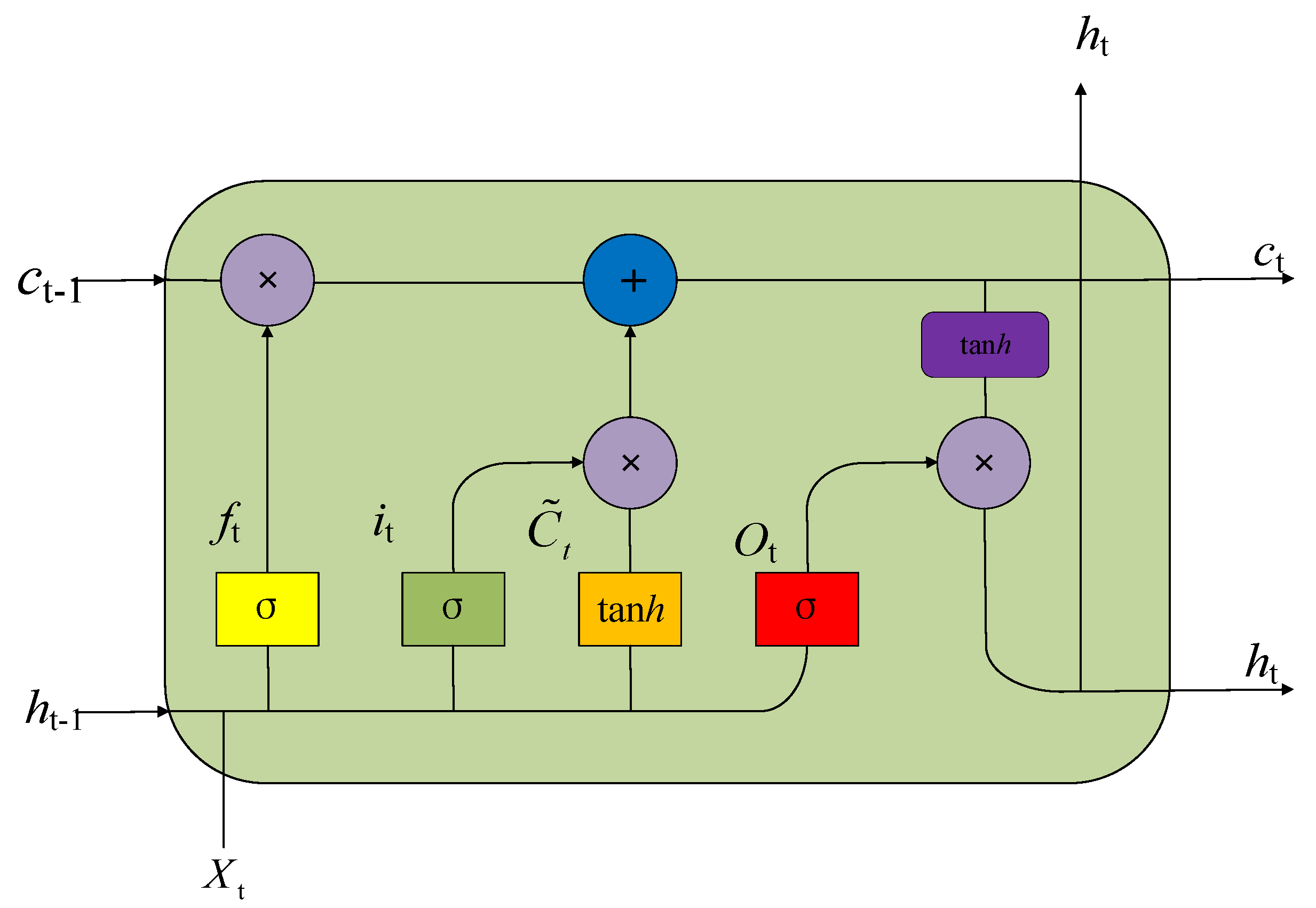
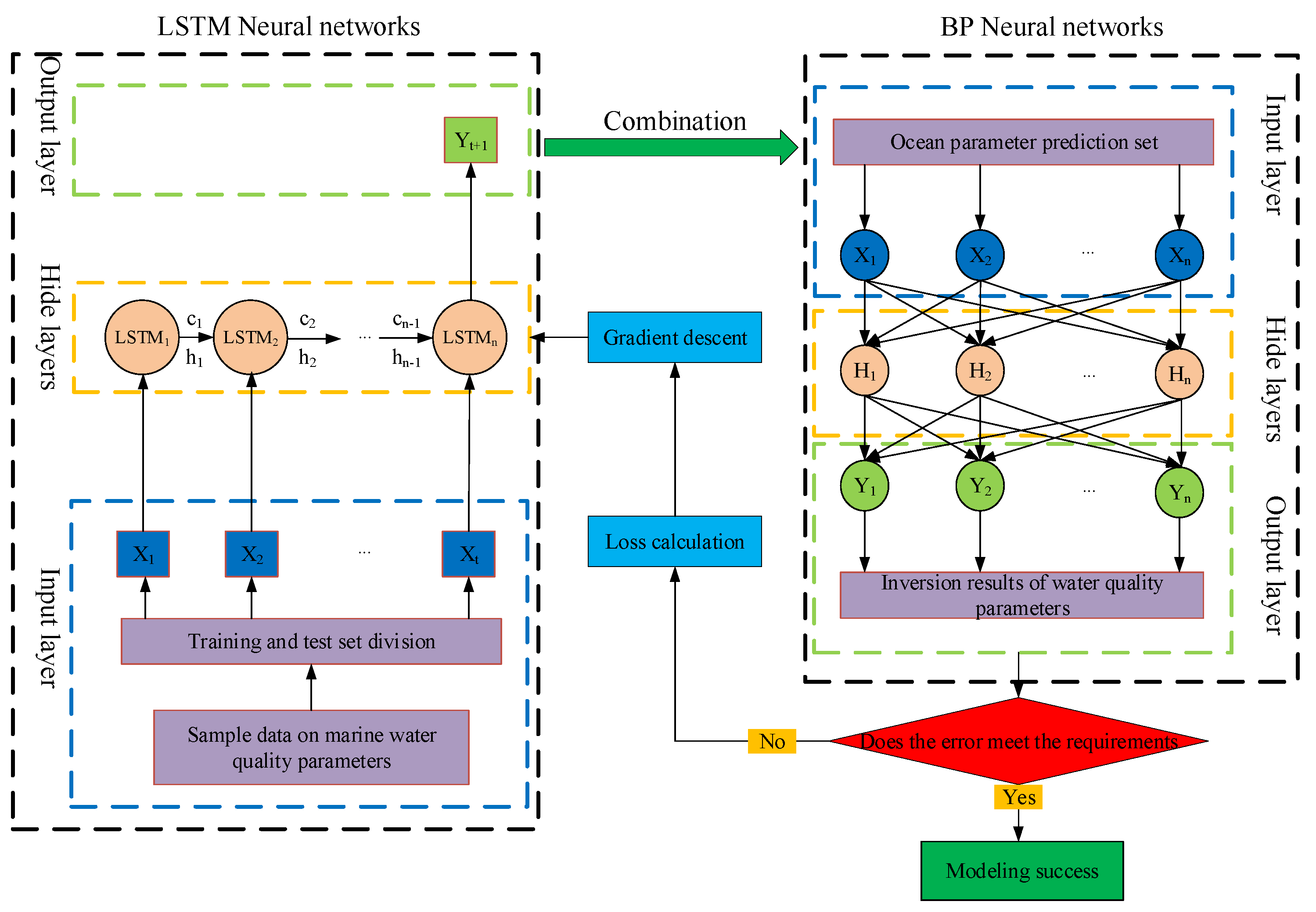
3.2. LSTM-BP Combination Model Construction

In this paper, the LSTM-BP model is used. LSTM is an improved deep neural network of the recurrent neural network, which belongs to the recurrent network [22]. As shown in Figure 3, it contains four elements: the forget gate, the input gate, the output gate, and memory cells of circular self-connection. The input of the forget gate is the input $x_t$ of the current unit and the hidden state $h_t{}_{-1}$ of the previous memory unit. This unit directly multiplies the control gate unit $C_{t-1}$ of the previous layer by $f_t$ to determine what information will be discarded; the input gate determines the information required for storage, and multiplies the retained new information $i_t$ with the control parameter $C_t$ formed by the new data to determine what data will be retained; the output gate will combine the output $o_t$ with the control gate unit to obtain the output result of the current hidden layer; the memory cells are used to update the operation $C_t$, which adds the memory gate unit and the forget gate unit to form the control gate unit to pass to the next stage [23].

$$\{\begin{array}{l}{f}_t=\sigma \left(W_f\times \left[h_{t-1},x_t\right]+b_f\right)\\ i_t=\sigma \left(W_i\times \left[h_{t-1},x_t\right]+b_i\right)\\ o_t=\sigma \left(W_o\times \left[h_{t-1},x_t\right]+b_o\right)\\ C_t=f_t\times C_{t-1}+i_t\times {\tilde{C}}_t\end{array}$$

(7)

In Equation (7), $h_{t-1}=o_{t-1}\times tan(C_{t-1})$; ${\tilde{C}}_t=tanh(W_c\times [h_{t-1},x_t]+b_c)$, $W_f$, $W_i$, $W_o$, $W_c$ are the weights of the forget gate, input gate, output gate, and memory cell, respectively; $b_f$, $b_i$, $b_o$, $b_c$ are the biases of the forget gate, input gate, output gate, and memory cell, respectively; $\sigma$ is the sigmoid function. LSTM is a special kind of recurrent neural network. The hidden layer of the original RNN has only one state, which is sensitive to short-term input, while LSTM adds a cell state to the hidden layer, improves the hidden layer of the RNN, and learns long-term information [24]. In the actual prediction, the historical data are used as the inputs of the LSTM network, and the state of the memory unit is continuously updated through the iterative calculation and training of the network, so as to predict future data changes through historical data.

A BP neural network is composed of forward propagation and back propagation. During forward propagation, the input sample data are passed to the input layer, processed by each hidden layer, and then the processed data are passed to the output layer [25]. If the output value of the output layer does not match the expected output value, the error is passed into back propagation. The back propagation of the error is reversed layer by layer, and the error is distributed to all the units of each layer so that each layer can obtain the error signal and correct the weight of the layer unit [26,27]. The weights are constantly adjusted, and the training is stopped when the number of iterations set by the experiment is reached or the output error is reduced to an acceptable range. Kolmogorov theoretically proved that given a sufficient number of hidden neurons, a neural network with one hidden layer can implement complex nonlinear mapping problems.

$$\{\begin{array}{l}h=f\left({\omega }_1^{T}x+b_1\right)\\ y=f\left({\omega }_2^{T}x+b_2\right)\end{array}$$

(8)

In Equation (8), $x$ is the input vector; $h$ is the hidden layer output vector; $y$ is the output layer vector; $f$ represents the activation function; ${\omega }_1$, ${\omega }_2$ represent the connection weights of the input layer and the hidden layer, respectively; $b_1$, $b_2$ represent the thresholds of the input layer and the hidden layer, respectively. The BP network training process is divided into forward propagation and backward propagation. The forward propagation process is used to calculate the output of the network, and the backward propagation is to adjust the network weight and bias according to the error feedback. After the network training is completed, the connection weights between neurons represent the specific knowledge of the diagnostic object.

In the modeling process of the LSTM-BP neural network, the training samples are divided into a training set and a verification set for training to determine hyperparameters such as neurons and network layers.

As shown in Figure 4, the normalized chlorophyll, turbidity, and dissolved oxygen data $X=\left\{X_1,X_2,\dots X_t\right\}$ are input into the LSTM neural network, and the time dimension characteristics of data changes are extracted by using the structural characteristics of the LSTM memory unit. The LSTM hidden layer includes $t$ time series LSTM cells, and the output of each LSTM memory cell in the hidden layer is $C=\left\{C_1,C_2\dots C_{n-1}\right\}$, $h=\left\{h_1,h_2\dots h_{n-1}\right\}$, where $C$, $h$ are the cell state and output of the hidden layer of the previous sample, respectively. Next, build a BP neural network, including an input layer, a hidden layer, and an output layer. The dimension of the input layer matches the output dimension of the hidden layer of the LSTM. The output of the LSTM hidden layer is used as the input data of the BP neural network to realize the data transmission from LSTM to BP. In this way, the BP neural network can further process the features extracted by the LSTM network. Specifically, the average error between the actual output of the BP network and the theoretical output is used as the error calculation formula to calculate the error, and the weight and bias of the LSTM network are adjusted through back propagation to reduce the error. In this way, the LSTM network can gradually learn better feature representations, thereby improving the performance of the LSTM-BP model.

In order to improve the performance of the model and prevent over-fitting problems, we will use Adam as the optimizer. Compared with the traditional gradient descent algorithm, it combines the advantages of Adagrad and momentum gradient descent algorithms and can adapt to sparse gradients and alleviate gradient oscillation problems. In addition, we will also use the dropout method to randomly deactivate the hidden layer neurons with a certain probability to improve the generalization ability of the model. In the pre-training phase, we found that the model works better when the input sequence length is 1, the dropout parameter is 0.2, the number of training iterations is 200, and the batch size is 50.

Through the training of the training samples, the important influencing factors such as the number of neurons and the number of network layers are determined. The appropriate number of neurons and the number of network layers have an important impact on the quality of the output of the neural network model. If the number is too small, the model is not easy to fit; if the number is too large, the generalization ability of the model will decrease. Therefore, we adopted the cross-validation method and tried a total of 16 model parameter combinations, including the number of LSTM neural network layers (2 layers, 3 layers), the number of neural units per layer of the LSTM neural network (10, 12), the number of network layers in the BP neural network (2 layers, 3 layers), and the number of units in each layer of the BP neural network (20, 24), from which the best combination is selected. It can be seen from

Table 1. Test results under 16 different model parameters.

Serial Number	LSTM Network Layers	LSTM Number of Neurons	BP Network Layers	BP Number of Neurons	MAE
1	2	10	2	20	0.0131
2	2	10	2	24	0.0097
3	2	10	3	20	0.0065
4	2	10	3	24	0.0039
5	2	12	2	20	0.0026
6	2	12	2	24	0.0016
7	2	12	3	20	0.0054
8	2	12	3	24	0.0058
9	3	10	2	20	0.0068
10	3	10	2	24	0.0072
11	3	10	3	20	0.0061
12	3	10	3	24	0.0146
13	3	12	2	20	0.0076
14	3	12	2	24	0.0153
15	3	12	3	20	0.0086
16	3	12	3	24	0.0073

that the model with the smallest MAE value of the sixth parameter combination performs best. Therefore, the LSTM-BP model in this paper chooses 2 layers of the LSTM neural network, 12 LSTM neural network gating neural units per layer, 2 layers of the BP neural network, and 24 BP neural network units per layer. The activation function uses the sigmoid function, the dropout parameter is 0.2, the maximum number of iterations is 200, the learning rate is 0.001, batch_size is 50, and the data input and output dimensions are 1.

3.3. Comparison of Model Settings

In order to verify the performance advantages of the LSTM-BP model, this study conducted comparative experiments with other models, including the LSTM time series forecasting neural network model, the PSO-BP combination model, and the SVM model in machine learning. The LSTM neural network adopts two hidden layer structures, the number of neurons in the hidden layer is 4 and 8, respectively, and the activation function adopts the sigmoid function. Set the dropout layer on the hidden layer with a dropout rate of 0.2. The maximum number of iterations is 200. The learning rate is 0.001. batch_size is 50. Use the Adam stochastic gradient descent algorithm. In the PSO-BP model, the number of particles is 20, the maximum inertia weight is 0.8, the minimum inertia weight is 0.4, the learning factor is 2.0, and the hidden layer of the BP neural network has 24 neurons. Set the dropout layer on the hidden layer. The dropout rate is 0.2, the maximum number of iterations is 200, the learning rate is 0.001, and batch_size is 50. In the selection of the kernel function of SVM, the Gaussian radial basis kernel function (GRBF) is selected, and the kernel parameter ${\sigma }^2$ and penalty parameter $C$ are determined as: ${\sigma }^2$ = 0.08, $C$ = 30. The software environment and platform during the experiment are shown in

Table 2. Experimental environment and platform.

Lab Environment	Specific Information
operating system	Windows10
processor	Intel(R) Pentium(R) CPU G3220 @ 3.00 GHz
Onboard RAM	8 G
programming language	Python3.6
development environment	Keras + TensorFlow/scikit-learn
development tools	Pycharm

.

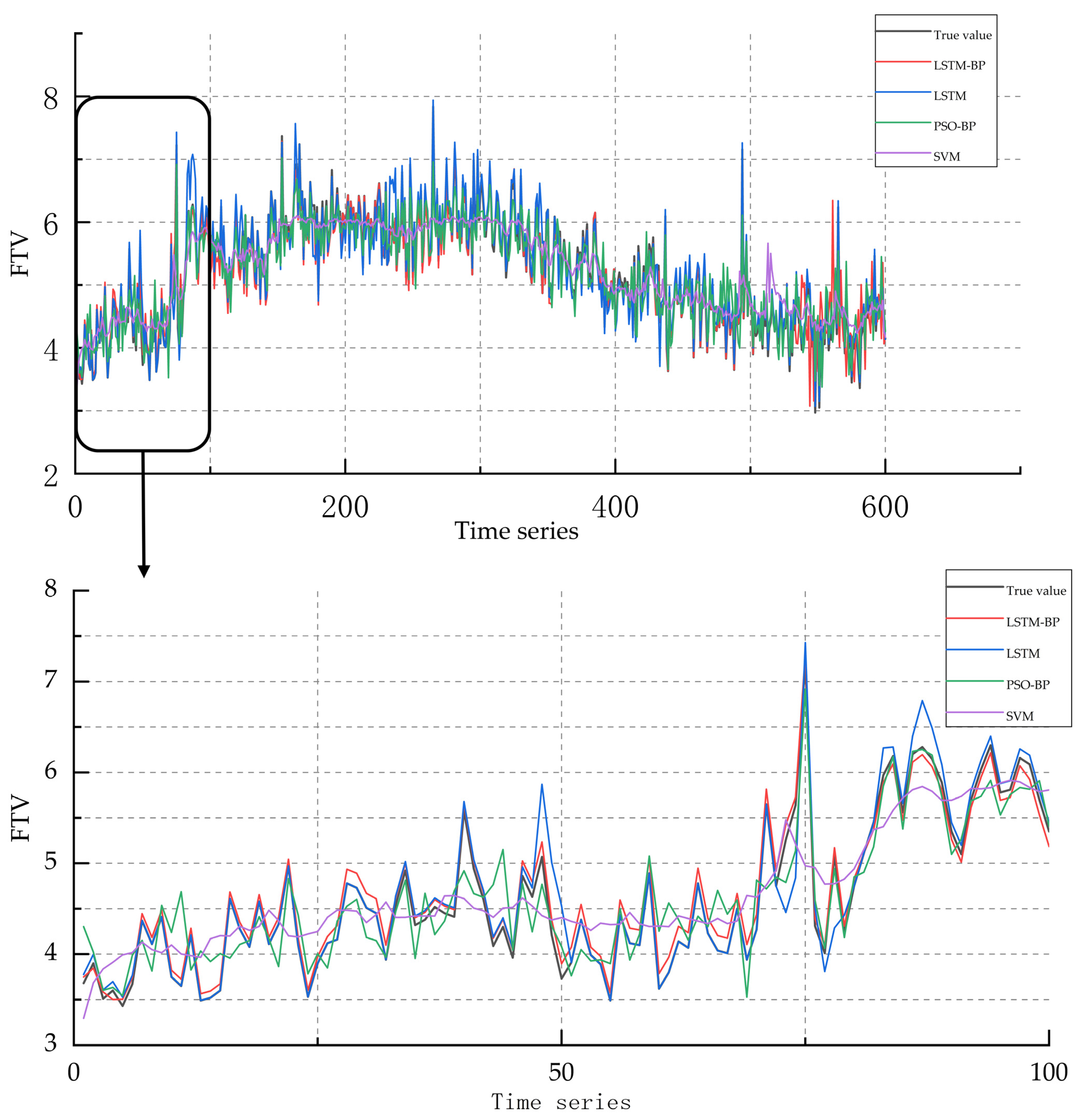
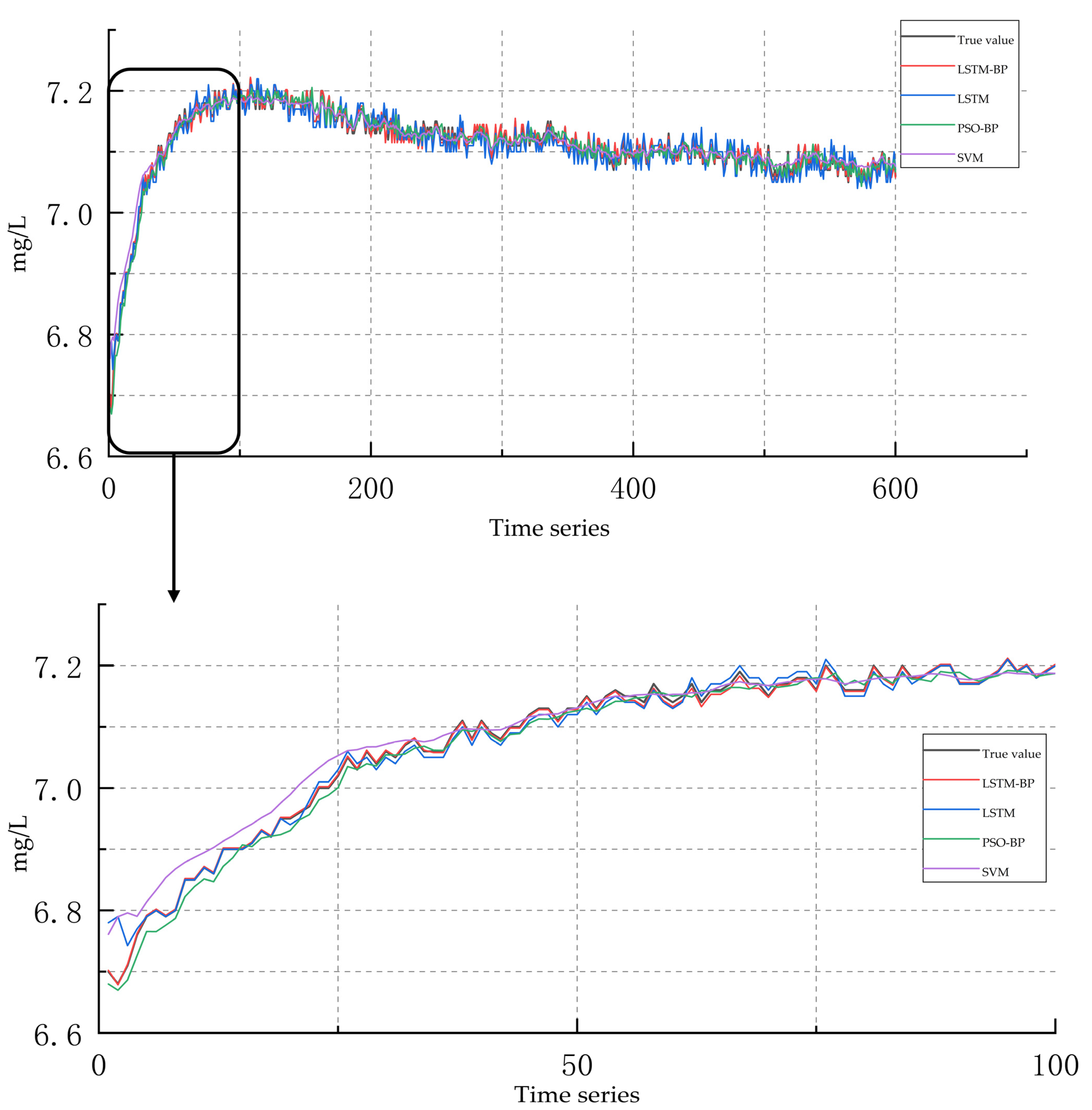
4. Analysis and Discussion of Experimental Results

We used the test data sets of the three parameters of chlorophyll, turbidity, and dissolved oxygen to conduct prediction tests on the LSTM-BP model, the LSTM neural network, the PSO-BP combined model, and SVM, respectively.

Figure 5, Figure 6 and Figure 7 show the prediction results of chlorophyll, turbidity, and dissolved oxygen on the four models of LSTM-BP, LSTM, PSO-BP, and SVM. The comparison shows that there is a large gap in the prediction results of different models. Among them, the black curve represents the original value, the red curve represents the predicted value of the LSTM-BP model, the blue curve represents the predicted value of the LSTM model, the green curve represents the predicted value of the PSO-BP model, and the purple curve represents the predicted value of the SVM model. From the prediction results, the SVM model only describes the trend of data changes, and its non-mapping ability is poor. Although the prediction accuracy of the PSO-BP model is stronger than that of the SVM model, there are still deficiencies in the time series prediction. The prediction accuracy of the LSTM model for a single value is not enough, local overfitting occurs, and the overall fitting degree is poor. Regardless of the number of time series points or the characteristic differences of water quality parameters, the LSTM-BP model performed best in predicting the three water quality parameters. In contrast, the predicted value of the LSTM-BP model is closer to the original value, and the overall fitting effect is better, which indicates that the LSTM-BP model can better learn the long-term dependencies in the time series, thereby improving the prediction accuracy.

Can be obtained from

Table 3. RMSE, MAE, and NSE of the three models (RMSE and MAE units 10⁻⁴).

	Chlorophyll			Turbidity			Dissolved Oxygen
	RMSE	MAE	NSE	RMSE	MAE	NSE	RMSE	MAE	NSE
LSTM-BP	36.64	23.50	0.967	2042.92	1214.25	0.876	52.69	38.28	0.971
LSTM	75.63	56.74	0.896	2578.36	1274.41	0.739	113.63	96.25	0.903
PSO-BP	125.26	87.63	0.853	2753.76	2003.65	0.686	119.45	101.62	0.874
SVM	157.16	114.58	0.761	4617.01	3275.73	0.577	151.40	112.75	0.765

. Regarding the NSE value: in the chlorophyll data prediction, the RMSE value of the LSTM-BP combined prediction model dropped by as much as 76.69%; in the turbidity data prediction, the RMSE value of the LSTM-BP combined prediction model dropped by as much as 55.75%; in the dissolved oxygen data prediction, the RMSE value of the LSTM-BP combined prediction model dropped by as much as 65.20%. Regarding the MAE value: in the chlorophyll data prediction, the MAE value of the LSTM-BP combined prediction model dropped by up to 79.49%; in the turbidity data prediction, the MAE value of the LSTM-BP combined prediction model dropped by 62.93%; in the dissolved oxygen data prediction, the MAE value of the LSTM-BP combined prediction model decreased by 66.05%. Regarding the NSE value: in the chlorophyll data prediction, the NSE value of the LSTM-BP joint prediction model increased by 21.30%; in the turbidity data prediction, the NSE value of the LSTM-BP joint prediction model increased by 34.13%; in the dissolved oxygen data prediction, the NSE value of the LSTM-BP joint prediction model increased by 21.22%. The predictive indicators RMSE and MAE of the LSTM-BP combined model were lower than those of the three control models, and NSE was higher than that of the three control models. It shows that LSTM is very sensitive to the choice of parameters, and the difference in parameter selection can easily lead to overfitting or underfitting of LSTM, thus affecting the prediction accuracy and generalization ability of LSTM. The SVM model can only capture linear relationships. The drastic changes in the environment make the water quality parameters non-linear and unstable, and there are complex coupling relationships among the water quality parameters, making it difficult to accurately predict the water quality parameters. The PSO-BP model is easy to fall into the local optimal solution, requires a large amount of training data and is sensitive to the initial weight, and the prediction time is longer than the other three models, so PSO-BP also has the disadvantages of high algorithm complexity and difficult parameter selection.

According to the results in Table 3, it can be seen that compared with the predictors of chlorophyll and dissolved oxygen, the predictors of turbidity are poor. This discrepancy may be due to the large magnitude variation of the dataset for turbidity. Turbidity is an index used to measure the content of suspended particulates in water, which is affected by many factors such as the concentration of suspended particulates and the flow of water. Due to the large variation in the turbidity data set, the LSTM-BP model may not be able to fully capture the characteristics and patterns of the data, and the model may pay too much attention to the data in a certain range while ignoring the data in other ranges, so the model’s prediction of the results as a whole is not ideal.

The LSTM-BP combined neural network is a neural network model that combines LSTM and BP. Different from traditional RNN, LSTM has memory cells and a gating mechanism, which can better capture long-term dependencies in time series data. The gating unit of LSTM controls the read and write operations of the storage unit through learnable parameters, enabling the network to selectively remember and forget information.

The BP neural network receives the output of the LSTM layer and performs further nonlinear transformation and mapping. Through the combination of multiple hidden layers and activation functions, the BP neural network can adapt to more complex nonlinear relationships and perform more accurate mapping. The BP neural network is trained through the back propagation algorithm, and the network parameters are updated according to the error between the predicted result and the real value. This process calculates the gradient layer by layer and updates the parameters through the chain rule so that the network can better approximate the nonlinear mapping function. Therefore, the LSTM-BP combination model can not only reflect the characteristics of time series but also has the ability of nonlinear mapping.

Although the LSTM-BP model can better predict the key water quality parameters of marine pastures, the model still has some room for improvement. First, the predictive performance of the method for datasets in different marine environments may vary, and model retraining and parameter adjustment may be required. Therefore, in future studies, the data can be updated in real-time to better predict key parameters of marine ranching. Secondly, when faced with a large data set, the model training time may be longer, and we need to find more efficient optimization algorithms to solve this problem.

5. Conclusions

Currently, deep learning is being applied more and more in the marine field, and neural networks are an ideal soft computing technique for modeling nonlinear and stochastic problems. Therefore, they have great potential in marine engineering. The data in this paper come from the Luhaifeng Marine Ranch in Qingdao City, Shandong Province, China, using three water quality parameters: chlorophyll, turbidity, and dissolved oxygen. Through LSTM-BP neural network combination model prediction, the prediction result is better than other models, and the RMSE and MAE are lower. Experiments show that the LSTM-BP model is suitable for the prediction of water quality parameters in marine pastures and provides a new method for the prediction of water quality parameters in marine pastures.

References

1. Hartman, S.E.; Bett, B.J.; Durden, J.M.; Henson, S.A.; Iversen, M.; Jeffreys, R.M.; Horton, T.; Lampitt, R.; Gates, A.R. Enduring science: Three decades of observing the northeast Atlantic from the Porcupine Abyssal Plain Sustained Observatory (PAP-SO). Prog. Oceanogr. 2021, 191, 102508. [Google Scholar] [CrossRef]
2. Chen, G.; Huang, B.X.; Chen, X.Y.; Ge, L.Y.; Radenkovic, M.; Ma, Y. Deep Blue AI: A new bridge from data to knowledge for the ocean science. Deep Sea Res. Part I Oceanogr. Res. Pap. 2022, 190, 103886. [Google Scholar] [CrossRef]
3. Tian, C.P.; Xu, Z.Y.; Wang, L.K.; Liu, Y.J. Arc fault detection using artificial intelligence: Challenges and benefits. Math. Biosci. Eng. 2023, 20, 12404–12432. [Google Scholar] [CrossRef] [PubMed]
4. Bartsev, S.; Saltykov, M.; Belolipetsky, P.; Pianykh, A. Imperfection of the convergent cross-mapping method. IOP Conf. Ser. Mater. Sci. Eng. 2021, 1047, 012081. [Google Scholar] [CrossRef]
5. Graf, R.; Zhu, S.L.; Sivakumar, B. Forecasting river water temperature time series using a wavelet–neural network hybrid modelling approach. J. Hydrol. 2019, 578, 124115. [Google Scholar] [CrossRef]
6. Wen, X.H.; Feng, Q.; Deo, R.C.; Wu, M.; Si, J.H. Wavelet analysis–artificial neural network conjunction models for multi-scale monthly groundwater level predicting in an arid inland river basin, Northwestern China. Hydrol. Res. 2016, 48, 1710–1729. [Google Scholar] [CrossRef]
7. Zhang, S.T.; Wu, J.R.; Jia, Y.G.; Wang, Y.G.; Zhang, Y.Q.; Duan, Q.B. A temporal LASSO regression model for the emergency forecasting of the suspended sediment concentrations in coastal oceans: Accuracy and Interpretability. Eng. Appl. Artif. Intell. 2021, 100, 104206. [Google Scholar] [CrossRef]
8. Gauch, M.; Kratzert, F.; Klotz, D.; Nearing, G.; Lin, J.; Hochreiter, S. Rainfall–runoff prediction at multiple timescales with a single long short-term Memory Network. Hydrol. Earth Syst. Sci. 2021, 25, 2045–2062. [Google Scholar] [CrossRef]
9. Chen, X.Y.; Chau, K.W. Uncertainty analysis on hybrid double feedforward neural network model for sediment load estimation with Lube Method. Water Resour. Manag. 2016, 33, 3563–3577. [Google Scholar] [CrossRef]
10. Clark, S.R.; Pagendam, D.; Ryan, L. Forecasting multiple groundwater time series with local and Global Deep Learning Networks. Int. J. Environ. Res. Public Health 2022, 19, 5091. [Google Scholar] [CrossRef]
11. Tang, Y.W.; Qiu, F.; Wang, B.J.; Wu, D.; Jing, L.H.; Sun, Z.C. A deep relearning method based on the recurrent neural network for land cover classification. GISci. Remote Sens. 2022, 59, 1344–1366. [Google Scholar] [CrossRef]
12. Song, W.; Fujimura, S. Capturing combination patterns of long- and short-term dependencies in Multivariate Time Series forecasting. Neurocomputing 2021, 464, 72–82. [Google Scholar] [CrossRef]
13. Guo, D.L.; Lintern, A.; Webb, J.A.; Ryu, D.; Bende-Michl, U.; Liu, S.C.; Western, A.W. A data-based predictive m-odel for spatiotemporal variability in stream water quality. Hydrol. Earth Syst. Sci. 2020, 24, 827–847. [Google Scholar] [CrossRef] [Green Version]
14. Lu, H.F.; Ma, X. Hybrid decision tree-based machine learning models for short-term water quality prediction. Chemosphere 2020, 249, 126169. [Google Scholar] [CrossRef]
15. Wang, H.; Wang, W.J.; Cui, Z.H.; Zhou, X.Y.; Zhao, J.; Li, Y. A new dynamic Firefly algorithm for demand estimation of water resources. Inf. Sci. 2018, 438, 95–106. [Google Scholar] [CrossRef]
16. Green, M.B.; Pardo, L.H.; Bailey, S.W.; Campbell, J.L.; McDowell, W.H.; Bernhardt, E.S.; Rosi, E.J. Predicting high-frequency variation in stream solute concentrations with water quality sensors and machine learning. Hydrol. Process. 2020, 35, 14000. [Google Scholar] [CrossRef]
17. Willard, J.D.; Read, J.S.; Appling, A.P.; Oliver, S.K.; Jia, X.W.; Kumar, V. Predicting water temperature dynamics of unmonitored lakes with meta-transfer learning. Water Resour. Res. 2021, 57, WR029579. [Google Scholar] [CrossRef]
18. Kargar, K.; Samadianfard, S.; Parsa, J.; Nabipour, N.; Shamshirband, S.; Mosavi, A.; Chau, K.W. Estimating longitudinal dispersion coefficient in natural streams using empirical models and machine learning algorithms. Eng. Appl. Comput. Fluid Mech. 2020, 14, 311–322. [Google Scholar] [CrossRef]
19. Ikotun, A.M.; Ezugwu, A.E.; Abualigah, L.; Abuhaija, B.; Heming, J. K-means Clustering Algorithms: A comprehensive review, variants analysis, and advances in the era of Big Data. Inf. Sci. 2023, 622, 178–210. [Google Scholar] [CrossRef]
20. Ismkhan, H.; Izadi, M. K-means-G*: Accelerating K-means clustering algorithm utilizing primitive geometric concepts. Inf. Sci. 2022, 618, 298–316. [Google Scholar] [CrossRef]
21. Dorabiala, O.; Kutz, J.N.; Aravkin, A.Y. Robust trimmed K-means. Pattern Recognit. Lett. 2022, 161, 9–16. [Google Scholar] [CrossRef]
22. Husein, M.; Chung, I.Y. Day-ahead solar irradiance forecasting for microgrids using a long short-term memory recurrent neural network: A deep learning approach. Energies 2019, 12, 1856. [Google Scholar] [CrossRef] [Green Version]
23. Aydın, H.; Orman, Z.; Aydın, M.A. A long short-term memory (LSTM)-based distributed denial of service (DDoS) detection and defense system design in Public Cloud Network Environment. Comput. Secur. 2022, 118, 102725. [Google Scholar] [CrossRef]
24. Tang, Y.Y.; Wang, Y.L.; Liu, C.L.; Yuan, X.F.; Wang, K.; Yang, C.H. Semi-supervised LSTM with historical feature fusion attention for temporal sequence dynamic modeling in Industrial Processes. Eng. Appl. Artif. Intell. 2023, 117, 105547. [Google Scholar] [CrossRef]
25. Ismael, M.; Mokhtar, A.; Farooq, M.; Lv, X. Assessing drinking water quality based on physical, chemical and microbial parameters in the Red Sea State, Sudan using a combination of water quality index and Artificial Neural Network Model. Groundw. Sustain. Dev. 2021, 14, 100612. [Google Scholar] [CrossRef]
26. Mouloodi, S.; Rahmanpanah, H.; Gohari, S.; Burvill, C.; Davies, H. Feedforward backpropagation artificial neural networks for predicting mechanical responses in complex nonlinear structures: A study on a long bone. J. Mech. Behav. Biomed. Mater. 2022, 128, 105079. [Google Scholar] [CrossRef] [PubMed]
27. Bogard, N.; Linder, J.; Rosenberg, A.B.; Seelig, G. A deep neural network for predicting and engineering alternative polyadenylation. Cell 2019, 178, 91–106.e23. [Google Scholar] [CrossRef]
Figure 1. Schematic diagram of the water quality monitoring system of Luhaifeng Marine Ranch.
Water 15 02760 g001
Figure 2. Structural diagram of the data acquisition platform.
Water 15 02760 g002
Figure 3. LSTM memory cell structure.
Water 15 02760 g003
Figure 4. LSTM-BP modeling process.
Water 15 02760 g004
Figure 5. Chlorophyll prediction curve.
Water 15 02760 g005
Figure 6. Turbidity prediction curve.
Water 15 02760 g006
Figure 7. Dissolved oxygen prediction curve.
Water 15 02760 g007