Surrogate-Based Multiobjective Optimization of Detention Pond Volume in Sponge City

Abstract

Detention ponds are effective structures for stormwater management in the urban drainage system of sponge cities. The pond size is taken as the decision variable, while the cost, total suspended solids (TSS), and catchment peak outflow (CPO) serve as the objectives for optimizing the detention pond volume. First, we randomly generated 10,000 pond areas and input them into the stormwater management model to simulate the time series of outflow and suspended solids concentration, thereby generating samples by combining the set of pond area, corresponding cost, TSS, and CPO. Then, two backpropagation neural network models (i.e., BPNN-TSS and BPNN-CPO) were trained, tested, and evaluated for predicting TSS and CPO, respectively. We employed them as surrogates and used the non-dominated sorting genetic algorithm-II to solve the optimization problem. The results showed: (1) The BPNN models accurately predicted TSS and CPO (determination coefficient 0.988~0.996, Nash–Sutcliffe efficiency 0.988~0.997), and efficiently substituted stormwater management model simulations for optimization purposes (residuals −18.49~28.10 kg and −0.45~0.29 m³/s). (2) For the Pareto solutions, the detention pond reduced TSS by 0~8.33% and CPO by 0~72.44% and delayed their peaks by 4~52 min; the reduction in TSS and CPO tends to grow as pond size increases, and CPO reduction exhibits a minor marginal effect. (3) The surrogate-based approach saves 90.03% runtime while preserving the quality of the Pareto solutions, verifying reliability.

1. Introduction

Detention ponds are structural control measures that regulate stormwater quantity and quality in urban drainage systems [1,2,3]. They allow suspended particles and adsorbable pollutants to settle during the stormwater detention residence [4] and reduce peak flows [5]. A successful design balances costs and other considerations, such as volume (or storage capacity) and operation rules [6]. Numerous empirical methodologies for pond volume design have been developed, including the unit area runoff method and the stormwater event, based on the inflow hydrograph method [7]. These methods are simple to implement, but they are susceptible to huge inaccuracies because they cannot capture the dynamic of stormwater outflows and quality in sponge cities, where low-impact development (LID) facilities are commonly used.

Consequently, hydrological simulations, which often consider the random nature of rainfall and the complexity of the pollutants removal mechanism, are used with optimization algorithms to design and operate the pond [8]. For instance, the stormwater management model (SWMM) is one of the most commonly used methods for continuously modeling an urban catchment’s water quantity and quality, including detention ponds [9]. Nevertheless, these simulation-optimization methods are computationally intensive and time-consuming for complex urban drainage systems [10,11]. Alternatively, surrogate models, or emulators, have excellent flexibility and generalization to the various nonlinear dynamics [12,13]. A surrogate model with sufficient details, satisfactory accuracy, and higher speed can substitute a physically based model partially or entirely. There are two types: lower-fidelity physically based surrogates reduce the resolution of the inputs, outputs, or internal processes of the original model, while response surface surrogates replace computationally expensive components with faster alternatives.

Therefore, we offer a surrogate-based framework for optimizing the volume of a sponge city’s detention pond based on experimental data from SWMM simulations. This paper focuses on the end-of-system detention pond for system-wide water quantity and quality control rather than on-site (i.e., distributed) detention ponds.

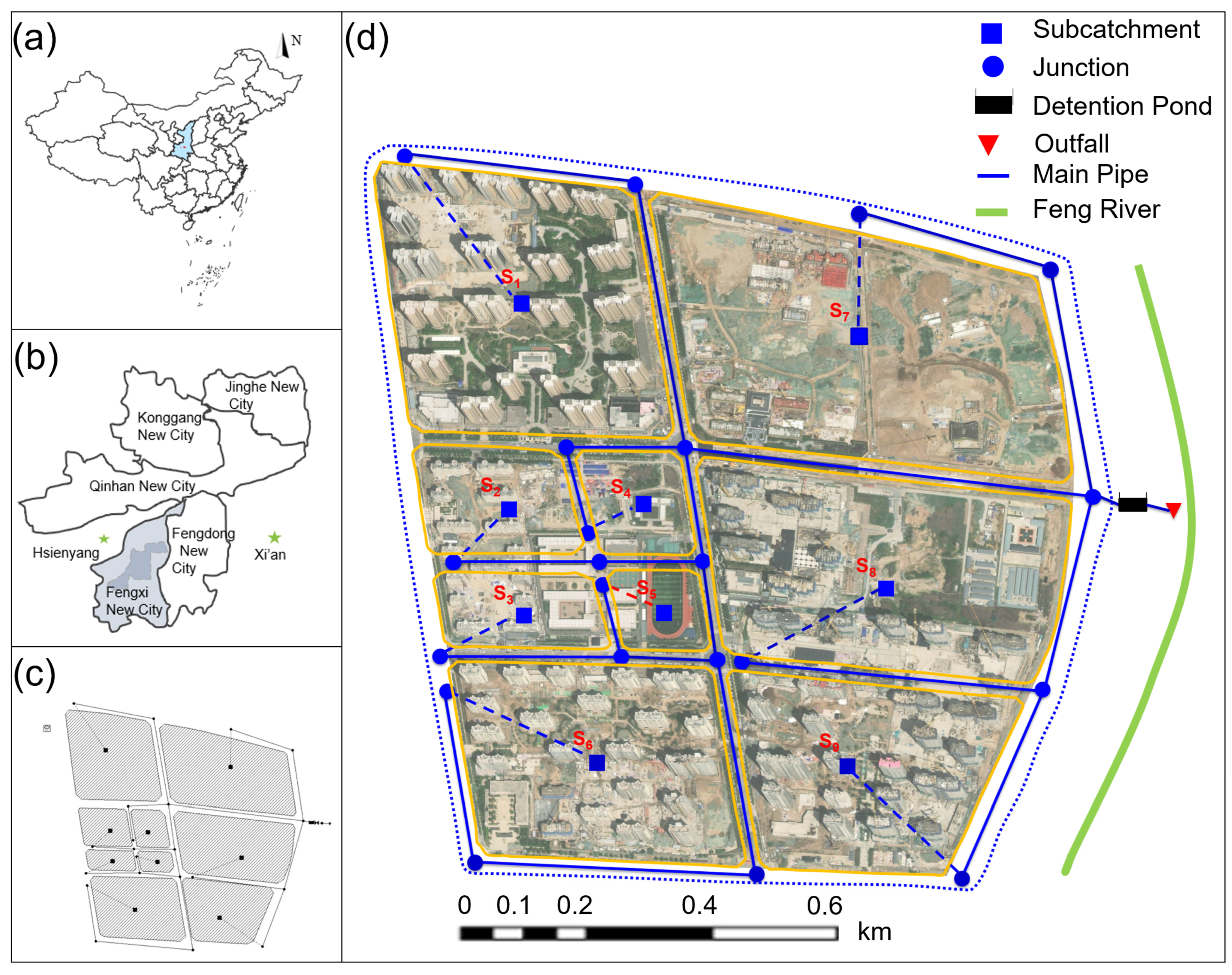
2. Study Area and Data

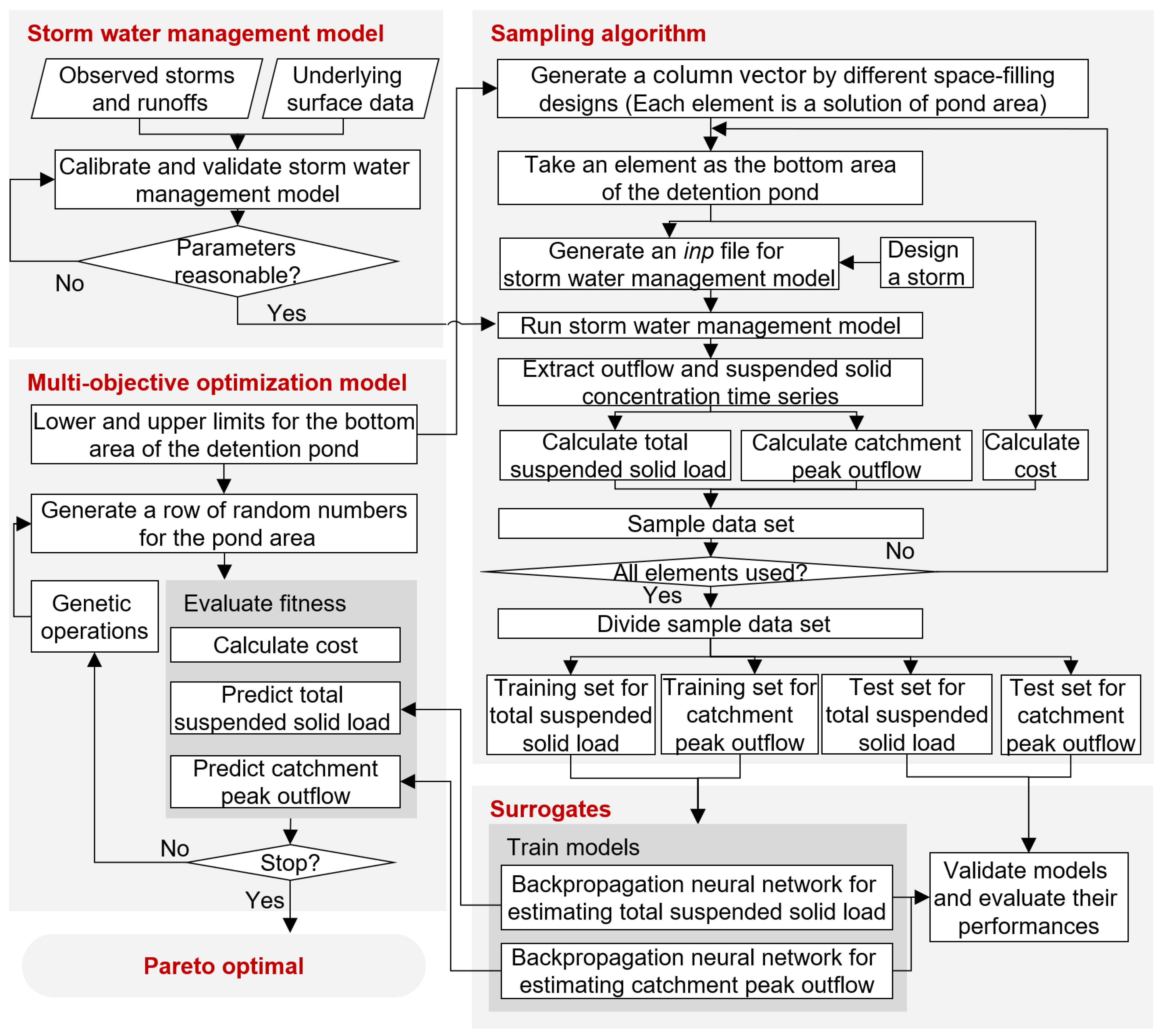
The study area is Weihe 8 (WR8, 845,335 m², Figure 1), an urban catchment in the sponge city pilot region of Fengxi New City (http://ecohydrology-ihp.org/demosites/view/1220, accessed on 15 June 2023) in China [14]. Its average annual precipitation is 552.0 mm, with 50–60% of the yearly precipitation falling between July and September. This region has a loess layer at an elevation between 380.5 and 384.3 m. The categories of land use are park-greenspaces, residential lands, transportation, educational institutions, industrial land, and undeveloped space. Through the outfall, the stormwaters of WR8 are discharged into the Fenghe River. Before 2014, most of Fengxi New City’s drainage systems were built to manage storms with 1-year or 2-year return periods; hence, storm-induced flooding often occurred due to inadequate drainage capacity. LID-based stormwater management technology [15], including green roofs, porous pavements, and bioretention cells, has been used to reduce stormwater runoff at the source in the pilot region since 2013.

WR8 was divided into nine subcatchments, 21 conduits, 22 nodes, and one outfall, based on the results of drainage system examinations. Most of the data, including rainfall, surface elevation, land use, storm-related facilities, and surface and pipe flow, were collected via the Fengxi Management Committee. We considered a terminal (end-of-system) detention pond [17] at the outfall for this study (Figure 2). It has a rectangular bottom, a circular orifice with a 1 m radius, and a maximum water depth of 5 m. Because total suspended solids (TSS) are typically connected with other pollution indicators and have been the primary water quality focus for urban runoff [18], we chose TSS as the evaluation index for water quality.

3. Methodology

The optimal volume of a detention pond is determined using a surrogate-based MOO framework based on a backpropagation neural network (BPNN) and SWMM (Figure 3). The procedure is as follows: (1) Generate the pond area randomly within the constraints to generate numerous SWMM input files. (2) Compute the pond’s life-cycle costs. (3) Simulate the time series of catchment outflow and suspended solids concentration at the outfall using SWMM, hence computing the total suspended solids load (TSS) and catchment peak outflow (CPO). (4) As a sample, assemble a set that includes the detention space, construction costs, TSS, and CPO. (5) Repeat the procedures above to obtain a sample set, then, divide it into a training set, a validation set, and a test set. (6) Train two BPNN models to predict the TSS and CPO separately. (7) Evaluate the two models’ performance. (8) Using the non-dominated sorting genetic algorithm-II (NSGA-II) [19,20], the surrogate-based MOO model is solved to obtain the Pareto solution set for the pond area. (9) Analyze the performance of the surrogate models and optimization results.

3.1. Chicago Design Storm

The Chicago storm time series, with a 2-year return period and 120 min duration, was utilized for the hydrologic and water quality simulations. The intensity–duration–frequency equation [21] for storms in the research region is:

$$i=\frac{A(1+C\lg T)}{({t+b)}^n}$$

(1)

where i is the average storm intensity, mm/min; A is the storm coefficient; C is the coefficient of variation; T is the return period, year; t is the storm duration, min; b is the duration correction factor; and n is the storm attenuation index, which relates to the return period. Here, A = 16.715, C = 1.1658, b = 16.813, and n = 0.9302. The Chicago storms’ rising and falling limbs are determined as follows:

$$i(t_b)=\frac{[\frac{(1-n)t_b}{r}+b]}{{(\frac{t_b}{r}+b)}^{n+1}}A(1+C\lg T)$$

(2)

$$i(t_a)=\frac{[\frac{(1-n)t_a}{1-r}+b]}{{(\frac{t_a}{1-r}+b)}^{n+1}}A(1+C\lg T)$$

(3)

where i(t_b) and i(t_a) are the time series of rainfall intensity for the rising and falling limbs, respectively; t_b and t_a are the times before and after the peak moment, respectively; and r is the time-to-peak coefficient, here, r = 0.35.

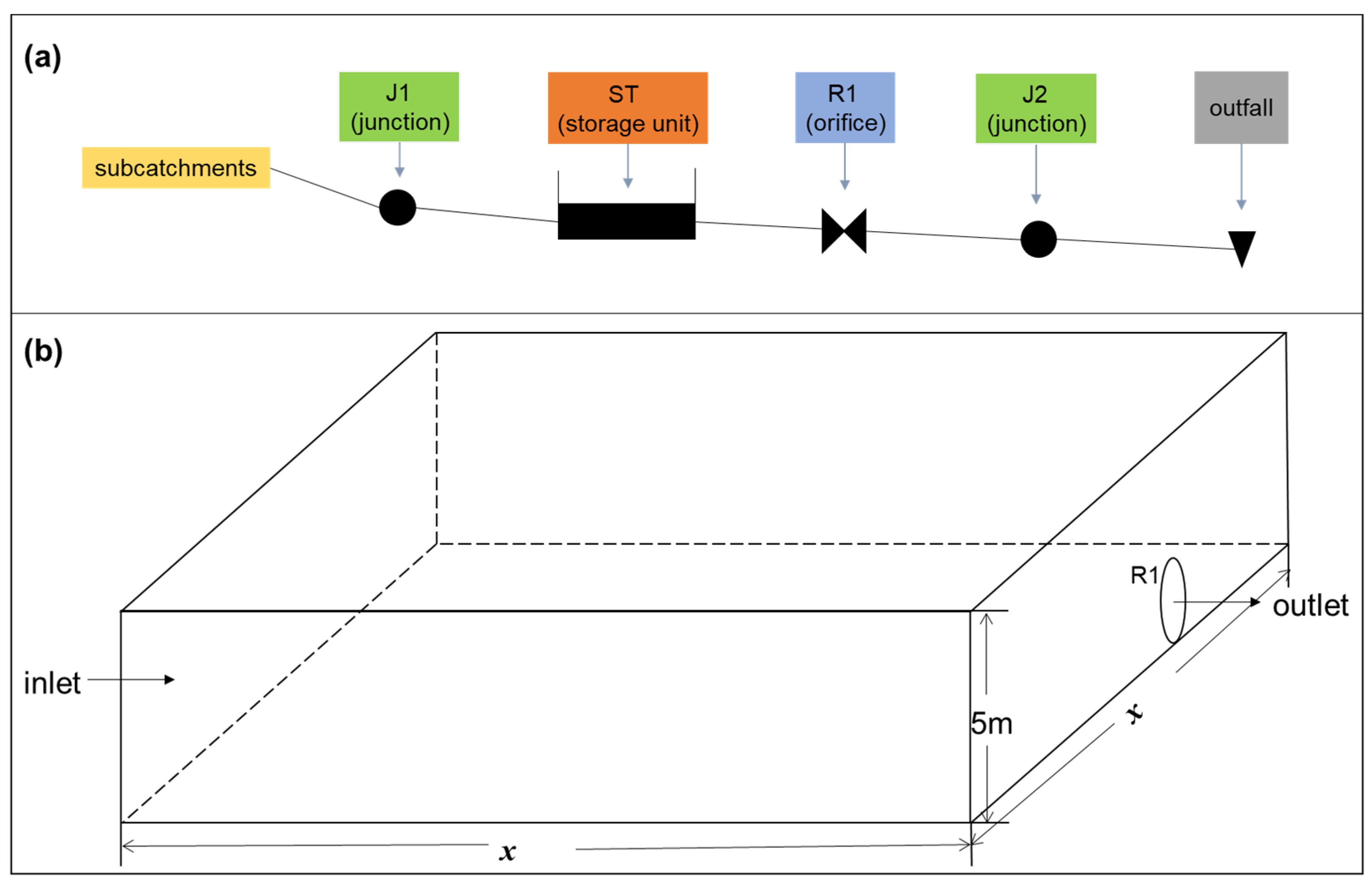
3.2. Detention Pond Simulation in Stormwater Management Model

Within each subcatchment, SWMM can mimic the processes of pollutant generation, inflow, and movement. It is not, however, supported by MATLAB calls. Therefore, we utilized MatSWMM, an alternative to SWMM established by [22]. MatSWMM is an open-source software program designed to analyze and build real-time control techniques for urban drainage systems. It includes control-oriented models, SWMM, and systematic-system edition functionalities. SWMM divides the research region into several subcatchments—hydrological land units that receive precipitation, produce runoff, and generate pollution loads [23]. The water quality module of SWMM divides the catchment into hydrological response units. For each hydrological response unit, SWMM specifies pollutant buildup and washoff models that take into account its characteristics. We selected the Horton infiltration model for the runoff simulation and the nonlinear reservoir model for the confluence simulation.

Table 1. Main parameters of catchment and detention pond in stormwater management model.

Parameter	Value
Catchment-related
Catchment slope (%)	0.5
Imperviousness (%)	0.76
Manning’s n for overland flow in impervious area	0.013
Manning’s n for overland flow in pervious area	0.15
Depression storage in impervious areas (mm)	1
Depression storage in pervious areas (mm)	3.2
Maximum infiltration rate of Horton curve (mm/h)	25.4
Minimum infiltration rate of Horton curve (mm/h)	3.56
Decay rate constant of Horton curve (1/h)	2
Last swept	1
Detention pond-related
Invert elevation (m)	380.58
Maximum depth (m)	5
Detention pond shape	Cube
Storage curve	TABULAR
Orifice type	SIDE
Orifice shape	CIRCULAR
Orifice diameter (m)	1
Discharge coefficient	0.65

lists the main hydrological, hydraulic, and detention pond parameters in SWMM. For additional information regarding the calibration and validation of SWMM, please consult Section 3.3 of the study by [14].

Buildup and washoff models were made by simplifying the natural system, which makes them especially good for specific catchments with clear boundaries [24]. How much pollution builds up depends on the antecedent dry days, the land use, and the sweeping frequency. The accumulation can be quantified by the number of pollutants per unit of area or boundary length. Here, we used the saturation equation [25] to figure out how much of a surface constituent was accumulating:

$$b=\frac{B_{\max }t}{K_B+t}$$

(4)

where b is the buildup mass per unit area, ML⁻²; B_max is the maximum buildup possible, ML⁻²; t is the accumulation time, T; and K_B is the half-saturation constant (i.e., the number of days when half of the B_max is reached), T. Washoff is the process of pollutants being dissolved and washed away by surface runoff. The exponential equation was used to describe the washoff:

$$w=K_W{q}^{N_W}{m}_B$$

(5)

where w is the washoff load, ML⁻¹; K_W is the washoff coefficient; q is the runoff rate per unit area, LT⁻¹; N_W is the washoff exponent; and m_B is the pollutant buildup in mass units, M.

Table 2. Pollutant buildup and washoff parameters for different land use types.

Parameter	Residence	Commercial Land	Greenbelt	Road
Area of land surface type (m2)	84,534	50,720	439,574	270,507
Proportion of the area of land use type to the total area	10%	6%	52%	32%
Maximum buildup possible (kg/hm2)	70	80	70	140
Days to reach half of the maximum buildup (day)	10	8	10	10
Washoff coefficient	0.001	0.001	0.050	0.001
Runoff exponent in washoff function	0.5	0.5	0.3	0.6

lists the values of the buildup and washoff parameters by land use.

In SWMM, a detention pond is represented as a storage unit node. By adding treatment functions to the properties of the node, SWMM can simulate the removal of pollutants in the pond’s outflow. We used the empirical exponential decay function to estimate how much solid matter falls to the bottom of a pond due to gravity.

$$C=10+(SS-10)\times e^{\frac{-0.01\times DT}{3600\times DEPTH}}$$

(6)

where C and SS are the concentration of suspended solids at the detention pond’s inlet and outlet, respectively, mg/L. DT is the evolution time step, s; and DEPTH is the water depth above the node’s bottom for the pond, m.

For a detention pond, the control rules (

Table 3. Water depth control rules of the detention pond.

Water Depth in the Detention Pond (m)	Orifice Opening Percentage
(0, 0.5]	0 (Fully close)
(0.5, 2]	20%
(2, 4]	40%
(4, 4.5]	60%
(4.5, 4.8]	80%
(4.8, 5]	100% (Fully open)

) alter the control object’s (here, an orifice) state by adjusting the attribute values (here, the opening degree or percentage [26]). For instance, when the water depth of the detention pond is less than 0.5 m, the opening of the orifice R1 is 0; that is, the orifice R1 is closed; when the water depth is between 0.5 m and 2 m, the opening of the orifice R1 is 20%.

As shown in Algorithm 1, we further programmed control rules for the detention pond using SWMM’s control editor [27]. The orifice R1 alternates between fully closed and fully open based on the water depth.

Algorithm 1. Control rule of detention pond in storm water management model.
1	RULE 1
2	IF NODE ST DEPTH > 0
3	AND NODE ST DEPTH ≤ 0.5
4	THEN ORIFICES R1 SETTING = 0
5	RULE 2
6	IF NODE ST DEPTH > 0.5
7	AND NODE ST DEPTH ≤ 2
8	THEN ORIFICES R1 SETTING = 0.2
9	RULE 3
10	IF NODE ST DEPTH > 2
11	AND NODE ST DEPTH ≤ 4
12	THEN ORIFICES R1 SETTING = 0.4
13	RULE 4
14	IF NODE ST DEPTH > 4
15	AND NODE ST DEPTH ≤ 4.5
16	THEN ORIFICES R1 SETTING = 0.6
17	RULE 5
18	IF NODE ST DEPTH > 4.5
19	AND NODE ST DEPTH ≤ 4.8
20	THEN ORIFICES R1 SETTING = 0.8
21	RULE 6
22	IF NODE ST DEPTH > 4.8
23	AND NODE ST DEPTH ≤ 5
24	THEN ORIFICES R1 SETTING = 1

3.3. Multiobjective Optimization

The bottom area of the detention pond is the decision variable of the MOO. We utilized three target functions competing with one another: the construction, maintenance, and management cost of the detention pond, TSS, and CPO [28,29].

$$\min f\left(x\right)=\left[COST\left(x\right),TSS\left(x\right),CPO\left(x\right)\right]$$

(7)

We computed the life-cycle cost of the detention pond using a single variable power function [30], ignoring the cost of the Chinese government’s developable land.

$$COST\left(x\right)=a{\left(xh\right)}^e+bx+g\left(x\right)$$

(8)

where x and h are the pond’s bottom area (m²) and water depth (m), respectively. Therefore, the pond volume is xh. a and b are constant coefficients related to the pond size and land cost, respectively; both depend on the economic level of WR8; here, a = 2000 and b = 500. The exponential index, e, represents the scale factor for urban economics, and e = 0.69 here. g(x) denotes the cost for initiating the pond construction, CNY. It is a choice function, as follows.

$$g(x)=\left\{\begin{array}{c}0,x=0\\ 50000,x\ne 0\end{array}\right.$$

(9)

The TSS (kg) load is calculated as follows.

$$TSS\left(x\right)={\sum }_{i=1}^t{c}_i{Q}_i$$

(10)

where c_i is the pollutant concentration at outfall in i-th time step, mg/L; Q_i is the average outflow rate at outfall in i-th time step, m³/s. The CPO (m³/s) is calculated as:

$$CPO\left(x\right)=\max Q_i$$

(11)

Site conditions constrain the pond’s size. In particular, the decision variables are controlled by minimum and maximum limits. These limits were determined based on the outcomes of numerous preliminary simulations with SWMM, the catchment’s total outflow, and a field investigation close to the study region.

$$100\le x\le 3000$$

(12)

The given multiobjective problem was resolved using NSGA-II [30], which is a rapid approach to solving many constrained problems. It incorporates elitism that prevents the deletion of a previously established Pareto optimal and employs explicit diversity-preserving mechanisms. A standard genetic algorithm (select, crossover, and mutation) is incorporated into NSGA-II, along with a non-dominated sorting and crowding distance. It is a commonly employed, computationally efficient, and resilient genetic algorithm that has proved its efficacy in several stormwater management experiments [20,31]. We utilized the gamultiobj function in MATLAB (https://ww2.mathworks.cn/products/matlab.html, accessed on 15 June 2023), which utilizes a variation of NSGA-II.

Table 4. Options of non-dominated sorting genetic algorithm-II in MATLAB.

Option	Value
Distance measure function	phenotype
Pareto fraction	0.35
Selection function	@selectiontournament
Constraint tolerance	10−3
Creation function	@gacreationuniform
Cross function	@crossoverintermediate
Cross fraction	0.8
Max generations	200
Function tolerance	10−4
Max stall generations	100
Max time (seconds)	Inf
Mutation function	@mutationadaptfeasible
Population size	1000

Notes: @ represents the calling of an embedded function in MATLAB.

contains the parameter values for the function. Using a single thread, all the computations were performed on a personal computer with an Intel Core i7-11700 processor (2.50 GHz) and 128 GB of random-access memory.

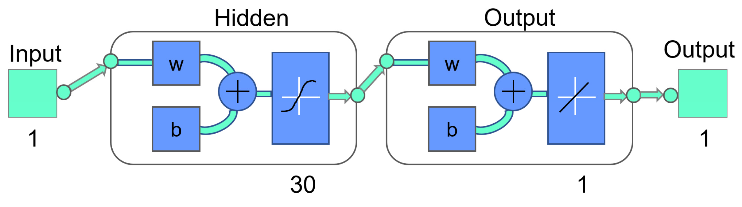
3.4. Surrogate Model

The approach comprises the following steps: (1) Randomly generate pond bottom areas using the Latin hypercube sampling technique. (2) Calculate each pond area’s TSS and CPO values using SWMM simulations. (3) Create samples by combining pond areas, TSSs, and CPOs. (4) Separate the sample set into 7:3 training and test sets. (5) Train, test, and evaluate BPNN models for surrogating SWMM.

The training data are evenly sampled for good generalization of the surrogate models. Four types of random points are generated using various space-filling strategies (Algorithm 2): 1000 points linearly spaced, 1000 points created uniformly, 4000 points generated using Latin hypercube sampling (LHS) [32,33], and 4000 points stratified by 20 folds (each generated using LHS). Then, these points were randomly divided into a training set and a test (holdout) set with a training ratio of 0.70.

Backpropagation neural networks (BPNN) are frequently used artificial neural networks composed of a feedforward network and backward error backpropagation [34]. BPNN has demonstrated promising results in several hydrology applications compared to other machine-learning algorithms [35]. A typical BPNN structure consists of input, hidden, and output layers. The hidden layers serve as the transfer function, establishing the input–output linkages. Each layer is composed of nodes, which are value-storing processing units. Weight and bias are modified in each iteration, based on the membership functions to approximate the intended outcome.

The following procedures are required to obtain optimal BPNN-TSS (BPNN model used to estimate TSS) and BPNN-CPO (BPNN model used to estimate CPO) models: (1) The size of the BPNN model’s hidden layers (ranging from 1 to 30) was determined. (2) BPNN-TSS (or BPNN-CPO) was constructed with a specific number of hidden layers using the Levenberg–Marquardt algorithm. (3) The 3000 trained BPNN-TSS (or BPNN-CPO) were compared using the root mean square error (RMSE, Equation (15)) to determine the best BPNN-TSS (or BPNN-CPO).

Algorithm 2. Pseudocode of sampling algorithm. nsam is the number of samples. LB and UB are the lower and upper boundaries for the pond area, respectively. P(t) is the rainfall depth during time ∆t. inp and out are the input and output files for the SWMM, respectively. xk is the pond area for the k-th sample. COSTk, TSSk, and CPOk are the life-cycle cost, TSS, and CPO for the k-th sample. C(k,t) is the average pollutant concentration and the average outflow rate at the outfall in t-th time step for the k-th sample, respectively. SAMk is the data point for the k-th sample.
1	Specify nsam, LB, and UB.
2	Get P(t)
3	Load inp
4	for k = 1 to nsam do
5	Randomly generate xk between LB and UB.
6	Calculate COSTk
7	Update the pond area in the CURVE section of inp with xk
8	Save the updated file as kth inp
9	Drive MatSWMM with kth inp
10	Save simulation results into kth out
11	Load kth out
12	end for
13	for k = 1 to nsam do
14	Get C(k,t) and Q(k,t)
15	Calculate TSSk
16	Calculate CPOk
17	Do SAMk = [xk, COSTk, TSSk, CPOk]
18	end for

The statistical error indices of the performance of BPNN-TSS and BPNN-CPO for training and testing must be addressed [36,37]. Thus, we used the mean absolute error (MAE), mean absolute percentage error (MAPE), root mean square error (RMSE), determination coefficient (DC), Nash–Sutcliffe efficiency coefficient (NSE), and percent bias (PBIAS). Lower MAE, MAPE, and RMSE values imply good simulation. The closer the values of NSE and DC are to 1, the higher the simulation quality. The PBIAS ranges from −∞ to +∞, with values close to zero indicating excellent performance. The error matrices are defined as follows:

$$\mathrm{MAE}=\frac{1}{n}\sum _{k=1}^n\left|y_k-\widehat{y_k}\right|$$

(13)

$$\mathrm{MAPE}=\frac{\sum _{k=1}^n\left|\frac{y_k-\widehat{y_k}}{y_k}\right|}{n}$$

(14)

$$\mathrm{RMSE}=\sqrt{\frac{\sum _{k=1}^n{\left(y_k-\widehat{y_k}\right)}^2}{n}}$$

(15)

$$\mathrm{DC}=\frac{\sum _{k=1}^n{\left(\widehat{y_k}-\overline{y}\right)}^2}{\sum _{k=1}^n{\left(y_k-\overline{y}\right)}^2}$$

(16)

$$\mathrm{NSE}=1-\frac{\sum _{k=1}^n{\left(y_k-\widehat{y_k}\right)}^2}{\sum _{k=1}^n{\left(y_k-\overline{y}\right)}^2}$$

(17)

$$\mathrm{PBIAS}=\frac{{\sum }_{k=1}^n{y}_k-\widehat{y_k}}{{\sum }_{k=1}^n{y}_k}$$

(18)

where k and n are the serial numbers of the sample and the sample size, respectively; y_k and $\widehat{y_k}$ are the k-th targets (i.e., TSS or CPO calculated by SWMM) and the k-th output (i.e., TSS or CPO predicted by BPNN), respectively; and $\overline{y}$ is the mean of y_k.

4. Results and Discussion

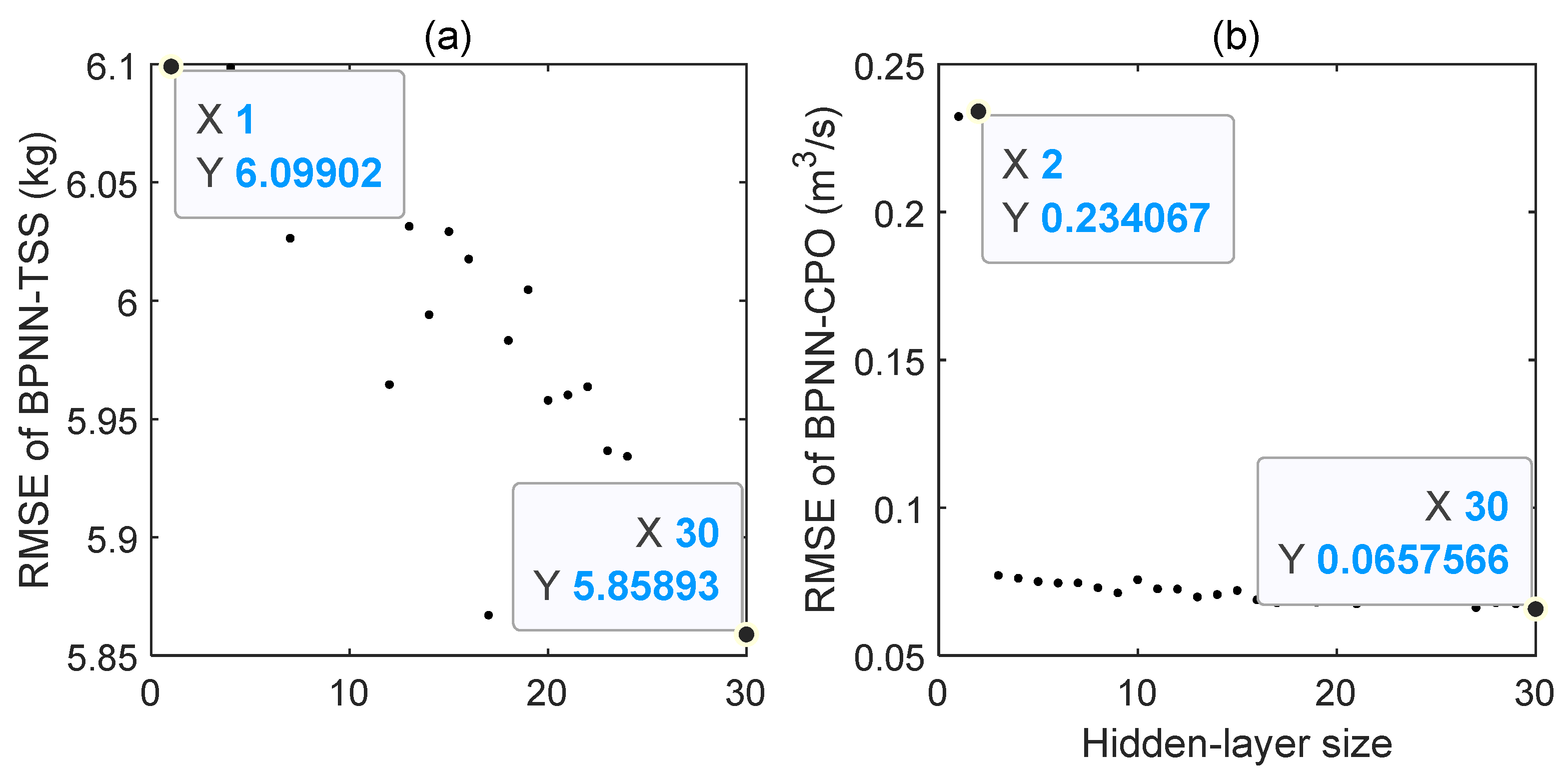
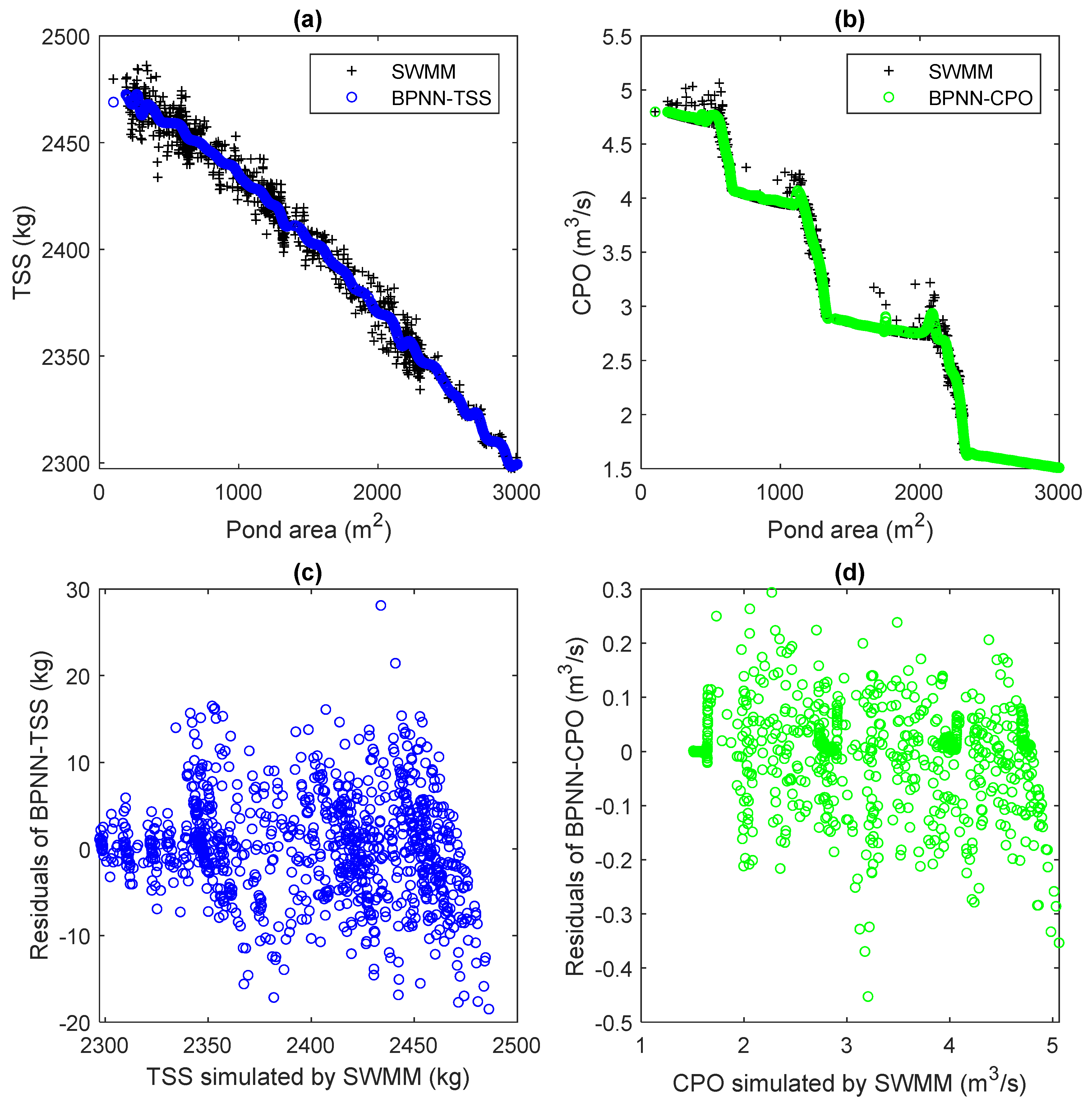
4.1. Performance of Surrogate Models

Figure 4 depicts the creation of 10,000 samples (pond areas, costs, TSSs, and CPOs). We observed that the costs grow as the pond area increases; in contrast, the TSS and CPO decrease. Due to the pond control rules based on water depth, the CPO reduces in a gradual manner (with a marginal effect).

According to the findings presented in Figure 5, the RMSE values of the BPNN-TSS and BPNN-CPO models with various hidden-layer sizes range from 5.86 to 6.10 kg and 0.07 to 0.23 m³/s, respectively. We found that having 30 hidden layers in our BPNN model produced the best results in terms of RMSE in the training phase, so we used that number. The architectures of the best BPNN models are depicted in Figure 6.

Figure 7 presents residual values of the BPNN-TSS and BPNN-CPO models in the test phase. The fact that the residuals of the BPNN-TSS and BPNN-CPO models varied from −23.59~26.58 kg and −0.28~0.47 m³/s, respectively, demonstrates that the BPNN models can accurately forecast TSS and CPO.

Table 5. Error statistics of optimal BPNN-TSS and BPNN-CPO models.

Indicators 1	MAE	MAPE	RMSE	DC	NSE	PBIAS
Training phase of BPNN-TSS	4.323	0.00179	5.859	0.990	0.988	−0.00003
Test phase of BPNN-TSS	4.392	0.00182	5.931	0.988	0.987	−0.00007
Training phase of BPNN-CPO	0.033	0.01017	0.066	0.996	0.997	−0.00002
Test phase of BPNN-CPO	0.034	0.01038	0.068	0.992	0.996	0.00041

Notes: ¹ Backpropagation neural networks, BPNN; catchment peak outflow, CPO; determination coefficient, DC; mean absolute error, MAE; mean absolute percentage error, MAPE; Nash–Sutcliffe efficiency, NSE; percent bias, PBIAS; root mean squared error, RMSE; total suspended solids load, TSS.

lists the training and generalization errors of the BPNN models. In the test phase of BPNN-TSS and BPNN-CPO, the MAE, MAPE, and RMSE were larger than they were in the training phase, while the DC and NSE were smaller, and the PBIAS was farther from 0. In addition, our statistical values outperformed the surrogate models based on polynomial regression models [38].

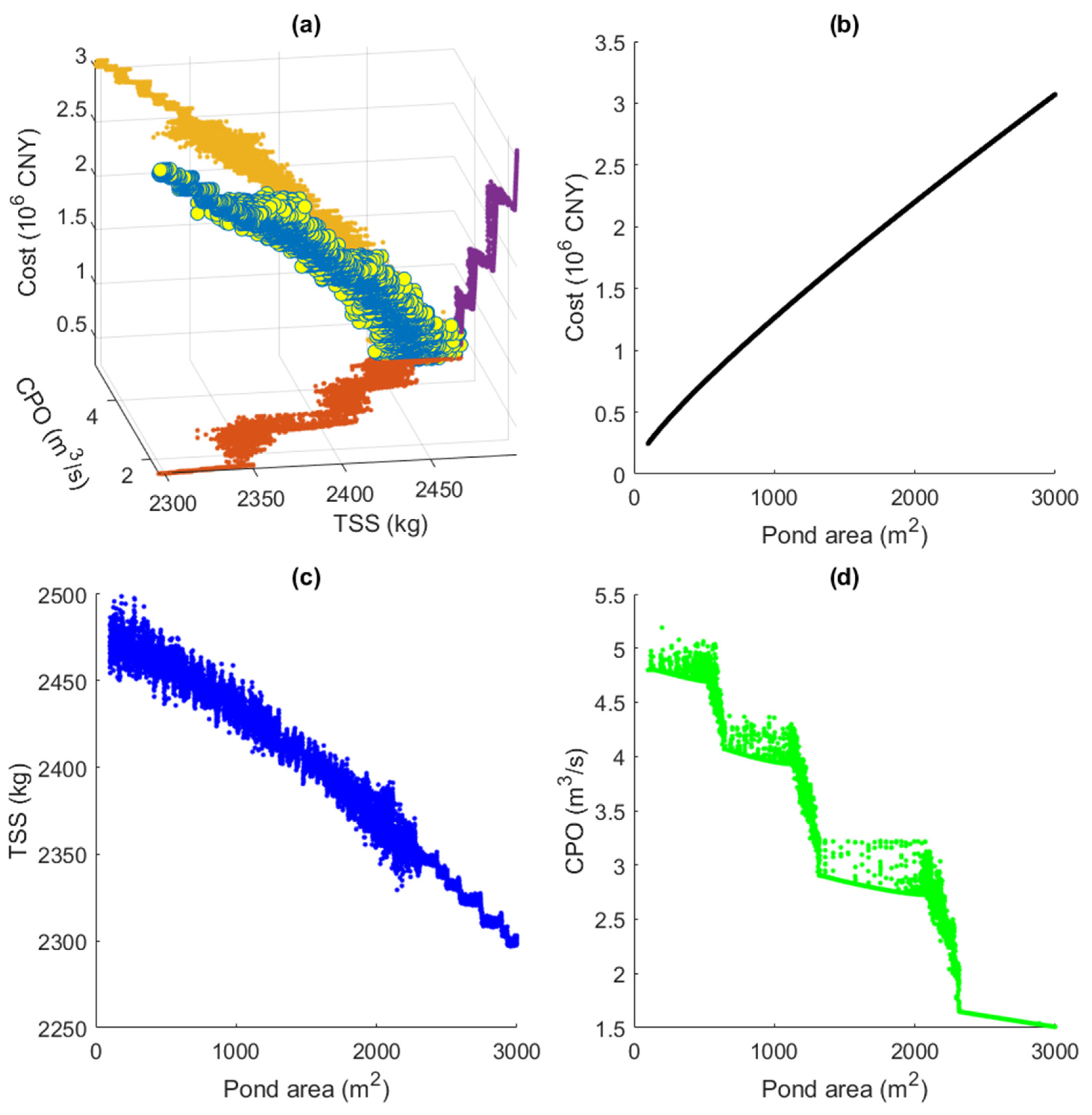
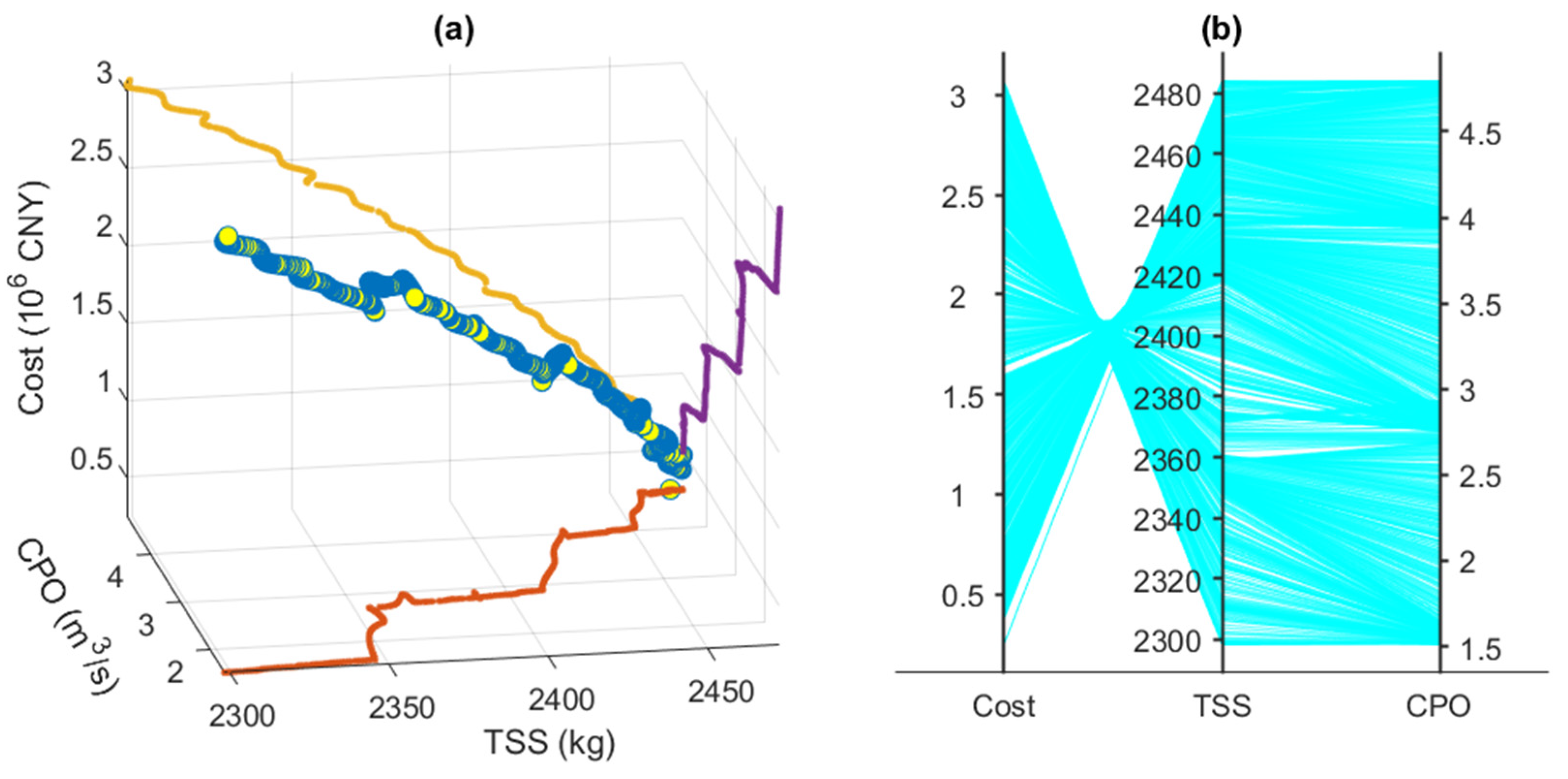
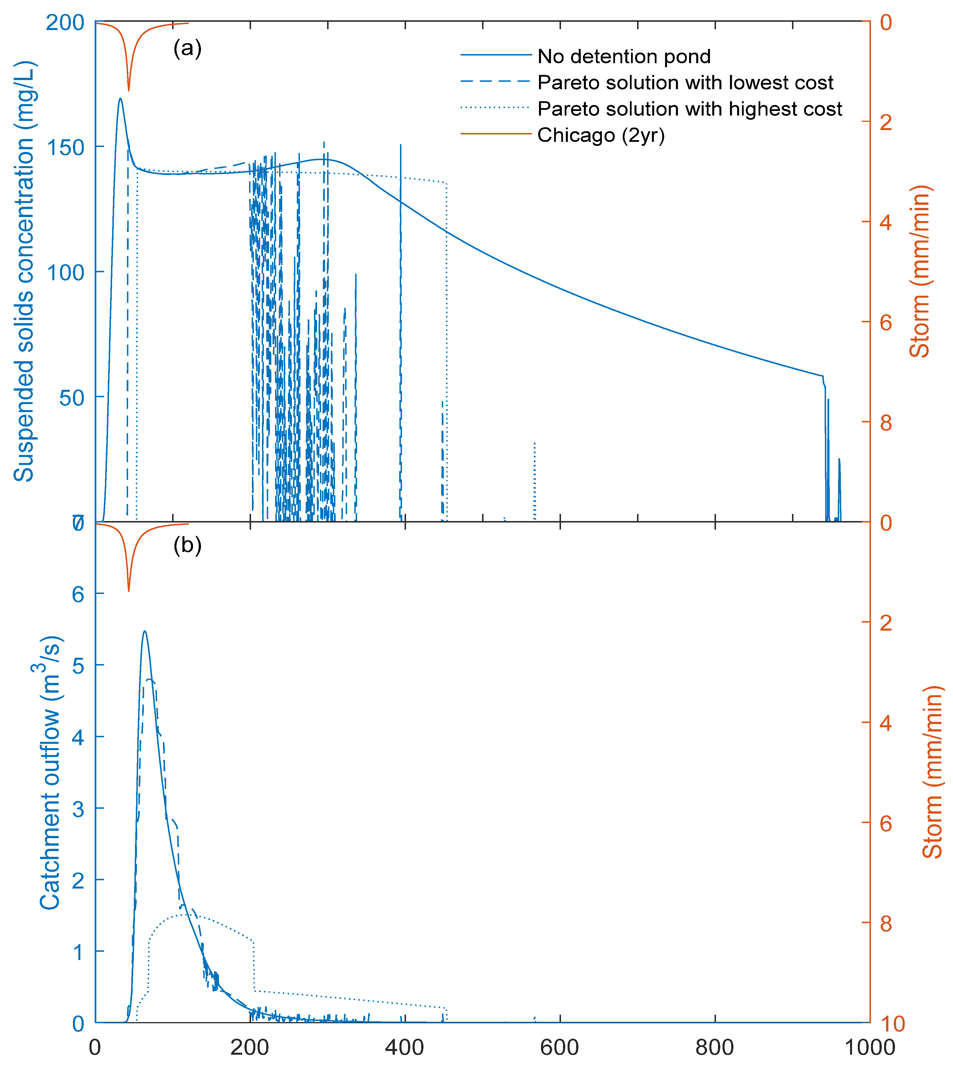
4.2. Effectiveness of Pareto Solutions

Figure 8 presents the front and parallel axis plots of the Pareto solutions. For the Pareto solutions, the cost ranges from 0.24 × 10⁶ to 3.07 × 10⁶ CNY, the TSS ranges from 2298.31 to 2472.62 kg, and the CPO ranges from 1.51 to 4.80 m³/s. Consequently, the optimal detention pond area could be chosen according to the decision-maker’s preference, thus determining the pond volume. For the Pareto fronts, constructing a pond with higher expenses likely contributes less TSS and CPO. There is a trade-off between price and TSS (or CPO). In most instances, reducing the TSS and CPO can be achieved by reducing the costs. The evaluation factors for tradeoffs may include planner demand, government budgets, etc. Investing more in detention ponds could reduce the installation of other infrastructure, such as LIDs. Therefore, stakeholder participation [39] is required for determining how to balance cost, TSS reduction, and CPO reduction.

Figure 9 displays hydrographs of the outflow and suspended solids concentration in the catchment with a detention pond volume of 0 m³ (scheme 0, no pond), 500 m³ (scheme 1, Pareto solution with the lowest cost; pond area is 100 m²), and 15,000 m³ (scheme 2, Pareto solution with the highest cost; pond area is 3000 m²), respectively. Scheme 0 (or 1, or 2) reached its maximum suspended solids concentration of 169.14 (or 152.58, or 141.63) mg/L at the 32nd (or 42nd or 54th) minute; scheme 0 (or 1, or 2) reached its peak outflow of 5.47 (or 4.80, or 1.51) m³/s at the 64th (or 68th, or 116th) minute. For schemes 1 and 2, the peak times of suspended solids concentration (or outflow) were 10 and 22 (or 4 and 52) minutes later than that of scheme 0, respectively.

Table 6. Statistics on schemes of no detention pond, Pareto solutions having lowest and highest costs.

Scheme	Pond Area (m2)	Cost (106 CNY)	Total Suspended Solids			Catchment Peak Outflow
			Mass (kg)	Reduction Rate	Reduction Unit Cost (106 CNY/kg)	Reduction Rate	Reduction Unit Cost (106 CNY/(m3/s))
0	0	0	2507.96	N/A	N/A	N/A	N/A
1	100	0.25	2479.77	1.12%	0.0089	12.29%	0.37
2	3000	3.07	2298.94	8.33%	0.0147	72.44%	0.78

details the three schemes’ (pond areas are 0, 100, and 3000 m²) costs, TSSs, and CPOs. We discovered that: (1) Scheme 2 has the highest cost and a substantial advantage in reducing TSS and CPO and delaying peaks. However, it is not cost-effective in TSS- and CPO-reduction. In contrast, scheme 1 is more cost-effective than scheme 2 in terms of reduction unit cost. Specifically, the CPO reduction in Figure 10b demonstrates a marginal effect. This result is consistent with that of Liu et al. (2016) [40], who observed that increased expenditures on LID facilities did not result in observable environmental benefits beyond a certain cost threshold. Therefore, the ideal decision should be based on a thorough cost-effectiveness study. (2) TSS reduction rates were lower than CPO reduction rates for a certain cost. This was anticipated, given that the detention pond’s default control rule is based on water depth rather than suspended solids concentration or residence time. Therefore, the control effect is more effective at reducing CPO than TSS.

As noted, the surrogate models performed admirably during the training and testing phases. There are still uncertainties caused by surrogates, which may impact the reliability of optimal solutions [33]. To simplify the problem, we did not quantify the uncertainty transmitted from intrinsic surrogate uncertainties into the pond volume optimization using an uncertainty analysis technique. Instead, we evaluated the BPNN-TSS and BPNN-CPO to validate the efficacy of the Pareto solutions in Figure 10. The BPNN-TSS residuals varied from −18.49 to 28.10 kg, and the BPNN-CPO residuals ranged from −0.45 to 0.29 m³/s, suggesting that their predictions were accurate. The Pareto solutions of the BPNN-based MOO are, hence, acceptable.

4.3. Computational Efficiency

In this study, the surrogate-based MOO search was terminated after 103 generations, namely, 103,000 evaluations of the objective function, given that the population size per generation is 1000. The runtime of an SWMM simulation with a pond area for calculating the TSS and CPO is about 3.572 s. The 10,000 SWMM simulations, which were necessary to generate the sample set for training and testing BPNNs, took around 3.57 × 10⁴ s (=3.572 × 10,000), followed by 7.664 s for learning the BPNN-TSS, 12.220 s for learning the BPNN-CPO, and 948.876 s for optimization searching. Therefore, a total runtime of 3.67 × 10⁴ s (=3.572 × 10⁴ + 7.664 + 12.220 + 948.876 s, about 10.19 h) was required for applying the proposed framework.

If the SWMM-based optimization (i.e., the objective function computes TSS and CPO through SWMM simulations) is performed, it would require 103,000 SWMM simulations, which would at least take around 3.68 × 10⁵ s (=103,000 × 3.572 s, about 102.20 h). In conclusion, the surrogate-based MOO framework can reduce the computational time by approximately 90.03%, making the proposed method more feasible. This outperforms the surrogate modeling using an adaptive neural network (74% time saving) [41].

5. Conclusions

We propose and validate a surrogate-based MOO framework for determining the size of a detention pond to minimize costs, TSS, and CPO. We conclude: (1) The BPNN models accurately predicted TSS and CPO and efficiently substituted SWMM simulations for optimization purposes with NSGA-II. (2) The detention pond can effectively reduce TSS and CPO and delay their peaks (the effect grows as pond size increases, exhibiting a minor marginal effect). (3) Compared to the simulation-optimization method, the approach saves much runtime while preserving the quality of the Pareto solutions, demonstrating the practicality of the approach.

This article tackles the MOO challenge of terminal detention ponds’ storage capacity in a sponge city with complex drainage systems. Future studies could be conducted on: judging the surrogate-based MOO’s applicability conditions, specifically, figuring out what scale or type of catchment is appropriate for using the surrogate model to compute the objective function of the optimization model rather than using a physical model; improving the physical interpretability and stability of the surrogate models by identifying key variables and mechanisms; and optimizing the volumes, locations, and real-time controls of the terminal and distributed detention ponds with complex features.

References

1. Cheng, M.; Qin, H.; Fu, G.; He, K. Performance evaluation of time-sharing utilization of multi-function sponge space to reduce waterlogging in a highly urbanizing area. J. Environ. Manag. 2020, 269, 110760. [Google Scholar] [CrossRef] [PubMed]
2. Gold, A.C.; Thompson, S.P.; Piehler, M.F. Seasonal Variation in Nitrate Removal Mechanisms in Coastal Stormwater Ponds. Water Resour. Res. 2021, 57, e2021WR029718. [Google Scholar]
3. Eckart, K.; McPhee, Z.; Bolisetti, T. Performance and implementation of low impact development—A review. Sci. Total Environ. 2017, 607–608, 413–432. [Google Scholar] [CrossRef] [PubMed]
4. Aldrees, A.; Dan’azumi, S. Application of Analytical Probabilistic Models in Urban Runoff Control Systems’ Planning and Design: A Review. Water 2023, 15, 1640. [Google Scholar]
5. Sharior, S.; McDonald, W.; Parolari, A.J. Improved reliability of stormwater detention basin performance through water quality data-informed real-time control. J. Hydrol. 2019, 573, 422–431. [Google Scholar] [CrossRef] [Green Version]
6. Behera, P.K.; Teegavarapu, R.S.V. Optimization of a Stormwater Quality Management Pond System. Water Resour. Manag. 2015, 29, 1083–1095. [Google Scholar]
7. Szeląg, B.; Kiczko, A.; Musz-Pomorska, A.; Widomski, M.K.; Zaburko, J.; Łagód, G.; Stránský, D.; Sokáč, M. Advanced Graphical–Analytical Method of Pipe Tank Design Integrated with Sensitivity Analysis for Sustainable Stormwater Management in Urbanized Catchments. Water 2021, 13, 1035. [Google Scholar]
8. Yang, S.N.; Chang, L.C.; Chang, F.J. AI-based design of urban stormwater detention facilities accounting for carryover storage. J. Hydrol. 2019, 575, 1111–1122. [Google Scholar] [CrossRef]
9. Yang, Y.Y.; Zhang, W.H.; Liu, Z.; Liu, D.F.; Huang, Q.; Xia, J. Coupling a Distributed Time Variant Gain Model into a Storm Water Management Model to Simulate Runoffs in a Sponge City. Sustainability 2023, 15, 3804. [Google Scholar] [CrossRef]
10. Zhang, G.S.; Hamlett, M.J.; Reed, P.; Tang, Y. Multi-Objective Optimization of Low Impact Development Designs in an Urbanizing Watershed. Open J. Optim. 2013, 2, 95–108. [Google Scholar] [CrossRef] [Green Version]
11. Oxley, R.L.; Mays, L.W. Optimization—Simulation Model for Detention Basin System Design. Water Resour. Manag. 2014, 28, 1157–1171. [Google Scholar] [CrossRef]
12. Tian, W.C.; Liao, Z.L.; Zhang, Z.Y.; Wu, H.; Xin, K.L. Flooding and Overflow Mitigation Using Deep Reinforcement Learning Based on Koopman Operator of Urban Drainage Systems. Water Resour. Res. 2022, 58, e2021WR030939. [Google Scholar]
13. Lund, N.S.V.; Borup, M.; Madsen, H.; Mark, O.; Mikkelsen, P.S. CSO Reduction by Integrated Model Predictive Control of Stormwater Inflows: A Simulated Proof of Concept Using Linear Surrogate Models. Water Resour. Res. 2020, 56, e2019WR026272. [Google Scholar]
14. Yang, Y.Y.; Li, J.; Huang, Q.; Xia, J.; Li, J.K.; Liu, D.F.; Tan, Q.T. Performance assessment of sponge city infrastructure on stormwater outflows using isochrone and SWMM models. J. Hydrol. 2021, 597, 126151. [Google Scholar] [CrossRef]
15. Duan, H.F.; Li, F.; Yan, H.X. Multi-Objective Optimal Design of Detention Tanks in the Urban Stormwater Drainage System: LID Implementation and Analysis. Water Resour. Manag. 2016, 30, 4635–4648. [Google Scholar]
16. Yang, Y.Y.; Li, Y.B.; Huang, Q.; Xia, J.; Li, J.K. Surrogate-based multiobjective optimization to rapidly size low impact development practices for outflow capture. J. Hydrol. 2023, 616, 128848. [Google Scholar] [CrossRef]
17. Liang, R.J.; Thyer, M.A.; Maier, H.R.; Dandy, G.C.; Di Matteo, M. Optimising the design and real-time operation of systems of distributed stormwater storages to reduce urban flooding at the catchment scale. J. Hydrol. 2021, 602, 126787. [Google Scholar]
18. Jefferson, A.J.; Bhaskar, A.S.; Hopkins, K.G.; Fanelli, R.; Avellaneda, P.M.; McMillan, S.K. Stormwater management network effectiveness and implications for urban watershed function: A critical review. Hydrol. Process 2017, 31, 4056–4080. [Google Scholar]
19. Deb, K.; Pratap, A.; Agarwal, S.; Meyarivan, T. A fast and elitist multiobjective genetic algorithm: NSGA-II. IEEE Trans. Evol. Comput. 2002, 6, 182–197. [Google Scholar]
20. Liu, D.; Huang, Q.; Yang, Y.Y.; Liu, D.F.; Wei, X.T. Bi-objective algorithm based on NSGA-II framework to optimize reservoirs operation. J. Hydrol. 2020, 585, 124830. [Google Scholar] [CrossRef]
21. Yang, Y.Y.; Xu, X.Y.; Liu, D.F. An Event-Based Stochastic Parametric Rainfall Simulator (ESPRS) for Urban Stormwater Simulation and Performance in a Sponge City. Water 2023, 15, 1561. [Google Scholar] [CrossRef]
22. Riaño-Briceño, G.; Barreiro-Gomez, J.; Ramirez-Jaime, A.; Quijano, N.; Ocampo-Martinez, C. MatSWMM—An open-source toolbox for designing real-time control of urban drainage systems. Environ. Modell Softw. 2016, 83, 143–154. [Google Scholar] [CrossRef] [Green Version]
23. Yu, J.J.; Qin, X.S.; Chiew, Y.M.; Min, R.; Shen, X.L. Stochastic Optimization Model for Supporting Urban Drainage Design under Complexity. J. Water Res. Plan Man 2017, 143, 05017008. [Google Scholar] [CrossRef]
24. Chaudhary, S.; Chua, L.H.C.; Kansal, A. The uncertainity in stormwater quality modelling for temperate and tropical catchments. J. Hydrol. 2023, 617, 128941. [Google Scholar] [CrossRef]
25. Rossman, L.A. Storm Water Management Model User’s Manual, Version 5.1; United States Environmental Protection Agency: Westlake, OH, USA, 2015.
26. Liang, R.J.; Maier, H.R.; Thyer, M.A.; Dandy, G.C.; Tan, Y.H.; Chhay, M.; Sau, T.; Lam, V. Calibration-free approach to reactive real-time control of stormwater storages. J. Hydrol. 2022, 614, 128559. [Google Scholar] [CrossRef]
27. Yazdi, J. Optimal Operation of Urban Storm Detention Ponds for Flood Management. Water Resour. Manag. 2019, 33, 2109–2121. [Google Scholar] [CrossRef]
28. Saadatpour, M.; Delkhosh, F.; Afshar, A.; Solis, S.S. Developing a simulation-optimization approach to allocate low impact development practices for managing hydrological alterations in urban watershed. Sustain. Cities Soc. 2020, 61, 102334. [Google Scholar] [CrossRef]
29. Luan, B.; Yin, R.X.; Xu, P.; Wang, X.; Yang, X.M.; Zhang, L.; Tang, X.Y. Evaluating Green Stormwater Infrastructure strategies efficiencies in a rapidly urbanizing catchment using SWMM-based TOPSIS. J. Clean. Prod. 2019, 223, 680–691. [Google Scholar] [CrossRef]
30. Li, F.; Duan, H.F.; Yan, H.X.; Tao, T. Multi-Objective Optimal Design of Detention Tanks in the Urban Stormwater Drainage System: Framework Development and Case Study. Water Resour. Manag. 2015, 29, 2125–2137. [Google Scholar]
31. Verma, S.; Pant, M.; Snasel, V. A Comprehensive Review on NSGA-II for Multi-Objective Combinatorial Optimization Problems. IEEE Access 2021, 9, 57757–57791. [Google Scholar] [CrossRef]
32. Lu, W.; Xia, W.; Shoemaker, C.A. Surrogate Global Optimization for Identifying Cost-Effective Green Infrastructure for Urban Flood Control With a Computationally Expensive Inundation Model. Water Resour. Res. 2022, 58, e2021WR030928. [Google Scholar] [CrossRef]
33. Zhang, W.; Li, J.; Chen, Y.H.; Li, Y. A Surrogate-Based Optimization Design and Uncertainty Analysis for Urban Flood Mitigation. Water Resour. Manag. 2019, 33, 4201–4214. [Google Scholar] [CrossRef]
34. Huang, C.L.; Hsu, N.S.; Wei, C.C.; Luo, W.J. Optimal Spatial Design of Capacity and Quantity of Rainwater Harvesting Systems for Urban Flood Mitigation. Water 2015, 7, 5173–5202. [Google Scholar] [CrossRef] [Green Version]
35. Zhang, P.P.; Cai, Y.P.; Wang, J.L. A simulation-based real-time control system for reducing urban runoff pollution through a stormwater storage tank. J. Clean. Prod. 2018, 183, 641–652. [Google Scholar] [CrossRef]
36. Stajkowski, S.; Hotson, E.; Zorica, M.; Farghaly, H.; Bonakdari, H.; McBean, E.; Gharabaghi, B. Modeling stormwater management pond thermal impacts during storm events. J. Hydrol. 2023, 620, 129413. [Google Scholar] [CrossRef]
37. Wang, J.; Guo, Y.P. Stochastic analysis of storm water quality control detention ponds. J. Hydrol. 2019, 571, 573–584. [Google Scholar] [CrossRef]
38. Lu, W.; Qin, X.S.; Yu, J.J. On comparison of two-level and global optimization schemes for layout design of storage ponds. J. Hydrol. 2019, 570, 544–554. [Google Scholar] [CrossRef]
39. Raei, E.; Alizadeh, M.R.; Nikoo, M.R.; Adamowski, J. Multi-objective decision-making for green infrastructure planning (LID-BMPs) in urban storm water management under uncertainty. J. Hydrol. 2019, 579, 124091. [Google Scholar] [CrossRef]
40. Liu, Y.Z.; Cibin, R.; Bralts, V.F.; Chaubey, I.; Bowling, L.C.; Engel, B.A. Optimal selection and placement of BMPs and LID practices with a rainfall-runoff model. Environ. Modell Softw. 2016, 80, 281–296. [Google Scholar] [CrossRef] [Green Version]
41. Yazdi, J.; Neyshabouri, S.A.A.S. Adaptive surrogate modeling for optimization of flood control detention dams. Environ. Modell Softw. 2014, 61, 106–120. [Google Scholar] [CrossRef]
Figure 1. Case study area (adapted from Yang et al., 2023 [16]). (a) Location: Shaanxi Province in China. (b) Pilot region in Fengxi New City, Xi’xian New Area. (c) Generalization map of WR8, the study site for hydrological simulations, extracted from stormwater management model. (d) Layout of drainage network in WR8.
Water 15 02705 g001
Figure 2. Diagram of detention pond. (a) Conceptual representation of terminal detention pond operated by an orifice control. (b) Three-dimensional shape.
Water 15 02705 g002
Figure 3. Surrogate-based multiobjective optimization framework for detention pond volume.
Water 15 02705 g003
Figure 4. (a) Life-cycle cost of the detention pond, TSS, and CPO for 10,000 simulation-generated samples using stormwater management model. Pond bottom areas versus corresponding (b) costs, (c) TSSs, and (d) CPOs. Yellow color indicates the trade-off between cost and TSS, red color indicates the trade-off between CPO and TSS, purple color indicates the trade-off between cost and CPO. Catchment peak outflow, CPO; total suspended solids load, TSS.
Water 15 02705 g004
Figure 5. (a) RMSE values of BPNN-TSS and (b) BPNN-CPO with different hidden-layer sizes in training phase. Backpropagation neural networks, BPNN; catchment peak outflow, CPO; root mean squared error, RMSE; total suspended solids load, TSS.
Water 15 02705 g005
Figure 6. Architecture of optimal BPNN-TSS and BPNN-CPO. Backpropagation neural network model, BPNN; catchment peak outflow, CPO; total suspended solids load, TSS.
Water 15 02705 g006
Figure 7. (a) Residuals of optimal BPNN-TSS and (b) BPNN-CPO in test phase. Backpropagation neural networks, BPNN; catchment peak outflow, CPO; stormwater management model, SWMM; total suspended solids load, TSS.
Water 15 02705 g007
Figure 8. Pareto solutions. (a) Pareto front of cost, TSS, and CPO. (b) Parallel axis plots of Pareto solutions. It can be employed to comprehend the tradeoffs between the three objectives. Yellow color indicates the trade-off between cost and TSS, red color indicates the trade-off between CPO and TSS, purple color indicates the trade-off between cost and CPO. Catchment peak outflow, CPO; total suspended solids load, TSS.
Water 15 02705 g008
Figure 9. Hydrographs of (a) outflow and (b) suspended solids concentration in catchment with a detention pond of different volumes. Namely, 0 m3 (scheme 0, no pond), 500 m3 (scheme 1, Pareto solution with lowest cost; pond area is 100 m2), and 15,000 m3 (scheme 2, Pareto solution with highest cost; pond area is 3000 m2).
Water 15 02705 g009
Figure 10. (a) TSS and (b) CPO simulated by BPNN and SWMM for Pareto solutions. Residuals of (c) BPNN-TSS and (d) BPNN-CPO for Pareto solutions. Backpropagation neural networks, BPNN; catchment peak outflow, CPO; stormwater management model, SWMM; total suspended solids load, TSS.
Water 15 02705 g010