VMD-GP: A New Evolutionary Explicit Model for Meteorological Drought Prediction at Ungauged Catchments

Abstract

Meteorological drought is a common hydrological hazard that affects human life. It is one of the significant factors leading to water and food scarcity. Early detection of drought events is necessary for sustainable agricultural and water resources management. For the catchments with scarce meteorological observatory stations, the lack of observed data is the main leading cause of unfeasible sustainable watershed management plans. However, various earth science and environmental databases are available that can be used for hydrological studies, even at a catchment scale. In this study, the Global Drought Monitoring (GDM) data repository that provides real-time monthly Standardized Precipitation and Evapotranspiration Index (SPEI) across the globe was used to develop a new explicit evolutionary model for SPEI prediction at ungauged catchments. The proposed model, called VMD-GP, uses an inverse distance weighting technique to transfer the GDM data to the desired area. Then, the variational mode decomposition (VMD), in conjunction with state-of-the-art genetic programming, is implemented to map the intrinsic mode functions of the GMD series to the subsequent SPEI values in the study area. The suggested model was applied for the month-ahead prediction of the SPEI series at Erbil, Iraq. The results showed a significant improvement in the prediction accuracy over the classic GP and gene expression programming models developed as the benchmarks.

1. Introduction

Minimizing the expected consequences of drought has become essential in the context of contemporary water resource planning and development [1,2]. In addition, it is anticipated that climate change may negatively affect available water resources [3,4]. It alters underlying dynamic patterns of both large-scale oceanic [5] and small-scale atmospheric events such as floods and droughts [6,7]. Local hydrometeorological patterns are also changing through growing urbanization, deforestation, and other anthropogenic activities [8,9,10]. Although climate change is mostly claimed as the main reason behind the increase in droughts’ frequency and intensity [11], the impacts of anthropogenic activities on large depletion in water storage and degradation in lakes’ levels must not be ignored [12,13].

Today, most communities have begun to develop drought monitoring and prediction systems so that they can adapt to its consequences in a more sustainable way. However, the task would be more challenging for the catchments suffering from scarce weather or hydrometric observatory stations [14]. To overcome this handicap in ungauged catchments, many studies adopted alternatives that use (i) nearby observatory records adjusted by spatial statistical techniques [15], (ii) remote sensing and satellite technology [16,17], and reanalysis products [18]. More recently, the use of global databases, such as Tropical Cyclone-related Precipitation Feature (TCPF), Data Observation Network for Earth (DataONE), the fifth generation ECMWF reanalysis for the global climate and weather known as ERA5, and Global Drought Monitoring (GDM) database have been recommended because of extensive spatiotemporal coverage and ease of access [18,19]. A comprehensive review of the applications of remote sensing methods in hydrological monitoring is available in Liu et al. [19]. For example, Xu et al. [20] and Seyyedi et al. [21] have used a reanalysis of precipitation data for flood risk modeling. The impact of reanalysis/global data on drought monitoring and prediction has previously been explored in part. Zhang et al. [22] utilized ERA5-land soil moisture data for agricultural drought assessment in southern China. Rakhmatova et al. [23] employed ERA-Interim and ERA5 reanalysis data for meteorological drought (hereafter MD) assessment in arid and semiarid regions of Uzbekistan. The authors demonstrated a high level of agreement between reanalysis data and observatory standardized precipitation evaporation index (SPEI) over Uzbekistan and neighboring regions. Vicente-Serrano et al. [24] demonstrated that reanalysis datasets offer a superb alternative to observational data that allow for better quantification of drought severity. More recently, Alee et al. [25] employed satellite images and GDM to retrieve the Normalized Difference Vegetation Index (NDVI) and SPEI across Erbil, respectively. Comparing the NDVI and SPEI time series, they concluded that MD is a trivial cause for spatial alteration in green areas over the Erbil Province, Iraq.

Due to economic and political challenges, Iraq suffers from discontinuing hydrometeorological measurements, and in many catchments, no reliable measuring devices are available [26]. Thus, hydrological analysis based on global data repositories creates reasonable benefits for the current circumstances [25]. Since the country’s food security depends mainly on its agricultural production, MD monitoring and prediction are of paramount importance for their sustainable development. Despite numerous studies on drought monitoring across Iraq (e.g., [27,28,29,30,31]), developing a drought prediction tool has rarely been studied in the relevant literature [32]. This is mainly due to the lack of long-term observatory data needed to identify the underlying complex pattern. Thus, this study proposes a new evolutionary model based on a global database for the automatic prediction of MD events in ungauged catchments. Although similar attempts have been conducted in the current literature [33], one question that remains unaddressed is the reliability of resolution and accuracy of global databases to be used on the catchment scale. To address the issue of resolution, we used the inverse distance weighting (IDW) interpolation method that gives more weight to the grids closer to the study area. From an accuracy point of view, i.e., potential noise available in the reanalyzed dataset, we suggested the integrated use of the variational mode decomposition (VMD) denoising technique with a rather new evolutionary modeling technique. Thus, the main contributions of this study are two-fold: (i) The research presents a novel evolutionary model for MD prediction using a global data repository. The model would be of paramount importance to be used in scarcely gauged or ungagged catchments; (ii) The VMD technique, for the first time, was coupled to state-of-the-art genetic programming (GP) to decompose row predictors, remove noise (high-frequency components), and select the best predictors instead of direct use of row global data. This may reduce inherited biases that are commonly available in fine-resolution reanalysis data when they are used at the catchment scale. The rest of this article is organized as follows. The study areas and the implemented data are described in Section 2. Section 3 elaborates on the method and the proposed methodology. Section 4 highlights the setup procedure for the proposed models, the evolved results, and the associated discussion. Section 5 concludes this paper with future scope.

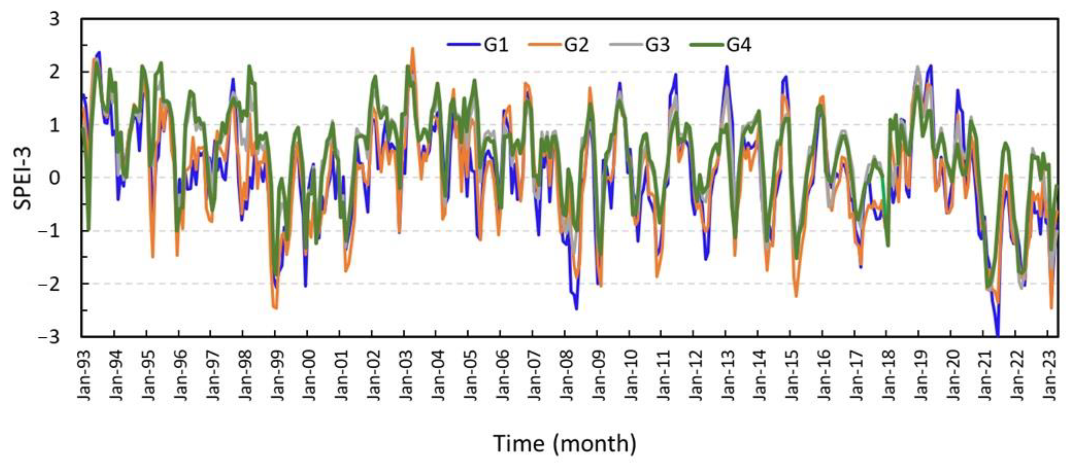
2. Study Area and Global Drought Data

The study area is the city of Erbil, also called Hawler (Figure 1; Lat = 36.19006° and long = 43.99303°), which is the capital and most populated city in the Kurdistan Region of Iraq. It lies in the Erbil Governorate. According to the annual weather statistics in the provinces of the Kurdistan Region provided by the Kurdistan Regional Statistical Office (KRSO 2021), there is only one meteorology station across the Erbil Governorate with a reliable measurement starting in 2012. During the past decade (2012–2021), the city has reached minimum and maximum precipitations equal to 196.2 mm and 733.8 mm in 2021 and 2018, respectively. The long-term observed minimum and maximum monthly average temperatures were 8.6 °C and 34.7 °C, respectively.

In this study, the SPEI-3 series, which represents water balance conditions over the past 3 months, was selected from the GDM repository (www.spei.es accessed on 30 May 2023) to construct the drought prediction models. The GDM database provides global long-time SPEI at several time scales with a half degree of spatial resolution. Thus, the global data from four grid points that are the nearest to the study area (see Figure 1 and

Table 1. Main characteristics of SPEI-3 series of the GDM nodes located near the Erbil.

Grid Point	Distance * (km)	Long.	Lat.	Min	Max	Mean
G1	24.22	43.75	36.25	−3.035	2.363	0.053
G2	22.30	44.25	36.25	−2.462	2.449	0.067
G3	53.60	43.75	35.75	−2.132	2.257	0.440
G4	52.85	44.25	35.75	−2.048	2.174	0.458

Note: * Direct distance between grid point and city center on the ground.

) were used to determine MD at the study area. Figure 2 depicts the SPEI-3 time series for the period between January 1993 and May 2023, and Table 1 summarizes their main statistical features. The mean SPEI values indicate the presence of higher wet conditions in lower latitudes (i.e., grid points G3 and G4). The underlying reason for selecting SPEI-3 in this study is the appropriateness of shorter-term accumulation periods for MD monitoring as well as measuring short-term humidity, subsurface water content, and impacts on streamflow of intermittent rivers existing around the study area.

3. Methods

3.1. The Standardized Precipitation and Evapotranspiration Index

The SPEI is a multiscale MD index that associates the cumulated water deficit ($D_i$) during a period of i months with the long-term cumulated water deficit for a given location at different accumulation periods. The SPEI was introduced by Vicente-Serrano et al. [19] as a measure of the MD regarding variation in both precipitation and temperature. Thus, water deficit, which is also called climatic water balance, is calculated through the subtraction of monthly potential evapotranspiration (PET) from total precipitation (P) during the same period.

$$D_i=P_i-PE{T}_i$$

(1)

Once the $D_i$ values are calculated, the values are aggregated at different time scales. Similar to the renowned standard precipitation index, the SPEI may be computed over short-time periods (up to 3 months), medium-term cumulated values (3–12 months), and long accumulation periods (12–24 months). Given $D_i$ series, the SPEI calculation is uniquely based on principles of probability. First, a theoretical distribution (e.g., three-parameter log-logistic distribution) is fitted to the desired $D_i$ series. Then, the SPEI is attained as the standardized values of the probability density function of $D_i$. In the original SPEI methodology, the Thornthwaite equation (to calculate PET) and log-logistic distribution (to normalize the index) are used, but there is a sensitivity of SPEI to PET calculation and probability distribution methods. Application of other methods, such as the modified Penman–Monteith equation and the Generalized Extreme Value distribution, have also been recommended.

The negative SPEI values refer to a dry spell, and the positive values refer to a wet event. The SPEI classification system, as defined by Danandeh Mehr et al. [34], categorizes the wet and dry conditions into three main classes of wet (i.e., SPEI > 1.0), near normal (i.e., −1.0 ≤ SPEI ≤ 1.0) and dry conditions (i.e., SPEI < −1.0). The dry condition, which is of interest in this study, is further divided into three subclasses: moderate drought (i.e., −1.42 ≤ SPEI ≤ −1.0); severe drought (i.e., −1.82 ≤ SPEI ≤ −1.43); and extreme drought (i.e., SPEI ≤ −1.83) events. For details on the calculations of the SPEI, the interested reader is referred to [19].

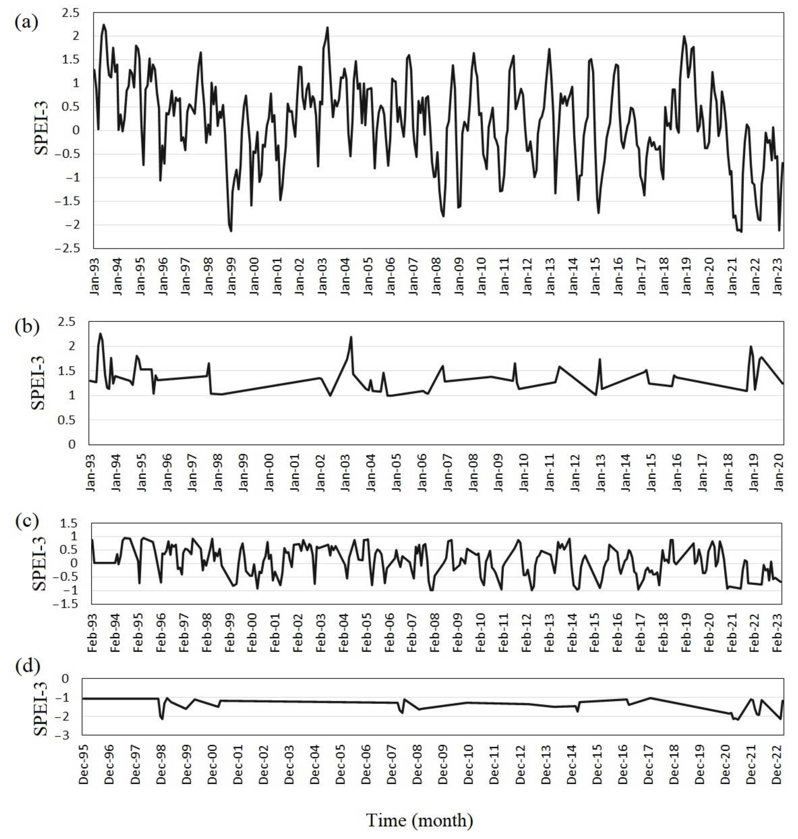
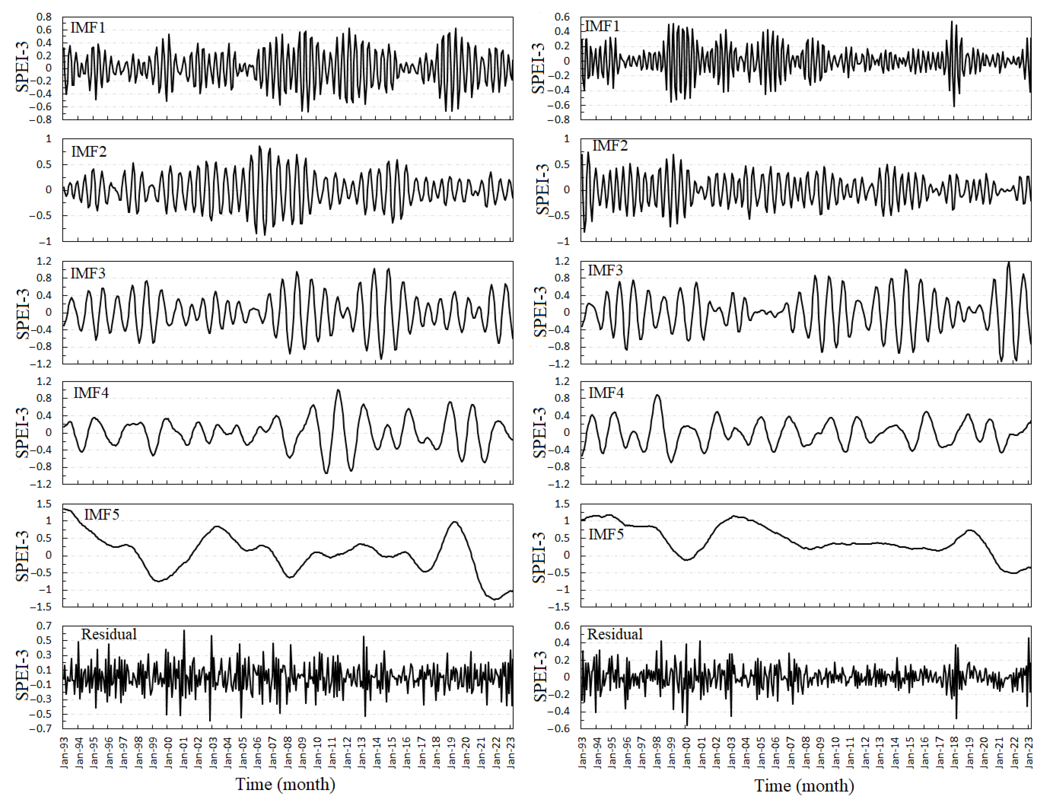
3.2. Variational Mode Decomposition (VMD)

The VMD [35] is a popular decomposition-based denoising technique used for signal processing and fault detection [36,37]. By defining a bandwidth constraint, the VMD non-recursively separates the complex signal into multiple stable intrinsic mode functions (IMFs) that oscillate around their central frequency. The VMD often outperformed the recursive-based decomposition technique, namely, the empirical mode decomposition, by demonstrating higher efficiency in removing high-frequency noises without diminishing much of the signal amplitude [38]. The VMD algorithm separates a noisy signal into a predefined number of IMFs, aka modes, that vibrate within a limited bandwidth in the spectral domain. Each of the modes (uk) would be most compact around its center of frequency (wk), which is defined along with the decomposition process. For a given SPEI series, the decomposition process is commenced by removing the negative frequency components based on Hilbert transform. Then, the frequency spectrum is altered to the baseband by merging with an exponential tuned to its attained frequency center. The bandwidth is estimated based on the Gaussian smoothness of the demodulated signal. After that, a constrained optimization problem is formulated (Equation (2)) based on the squared L2-norm of the gradient. The problem can be solved via the iterative alternate direction method of multipliers described in Dragomiretskiy and Zosso [35].

$$\begin{array}{c}\min \\ u_k,w_k\end{array}=\left\{\sum _k{‖{\mathsf{\partial }}_t\left[\left(\delta \left(t\right)+\frac{j}{\pi t}\right)\ast u_k\left(t\right)\right]e^{-j{w}_{k}t}‖}_2\right\}$$

(2)

where k is the scale number that indicates the total number of IMFs; u_k is the kth mode; w is the frequency; δ is the Dirac distribution; the asterisk sign represents the convolution operator, and ${\mathsf{\partial }}_t$ stands for partial derivative respect to time t.

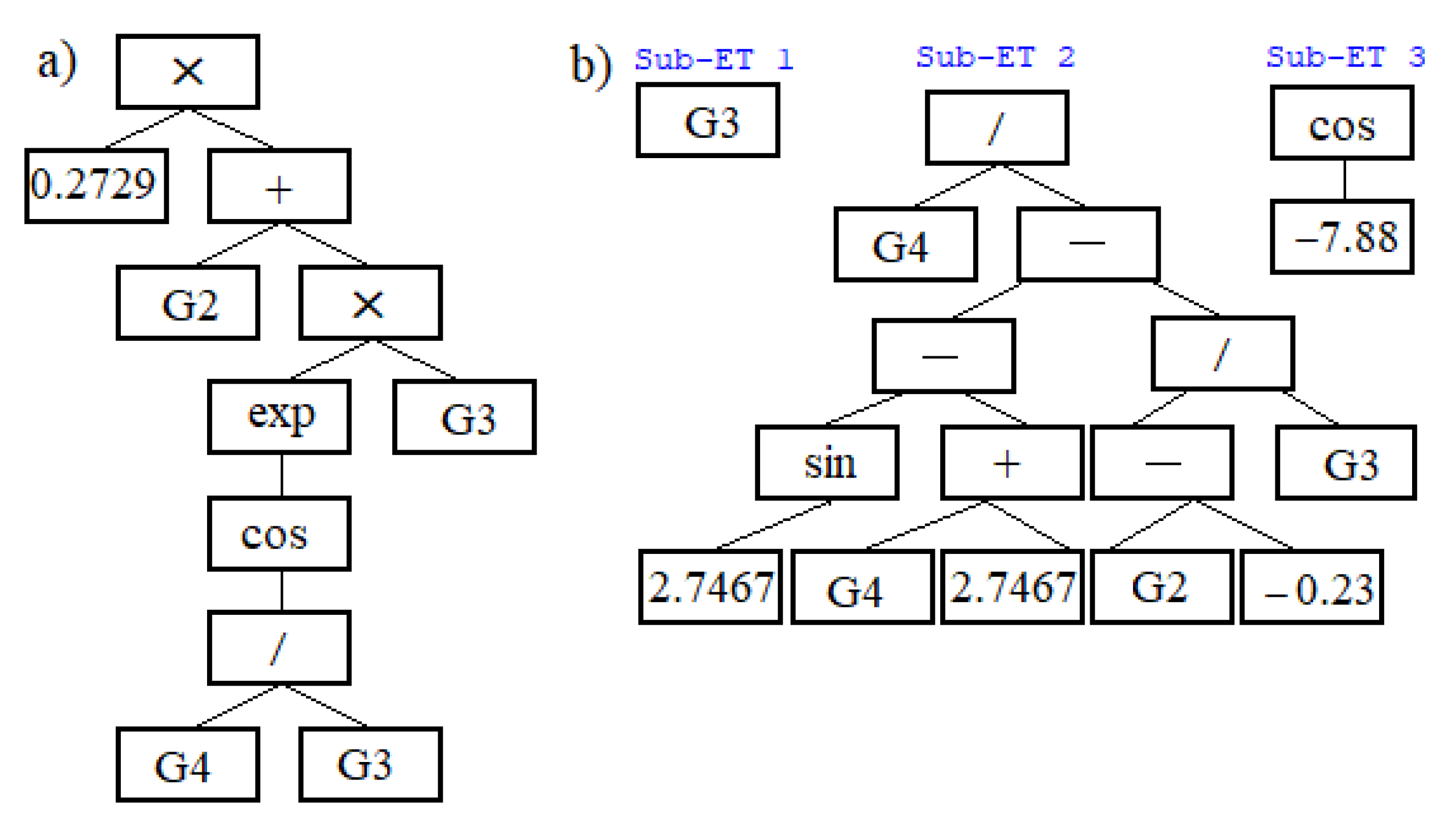
3.3. State-of-the-Art Genetic Programming and Gene Expression Programming

The GP is an evolutionary symbolic regression technique that automatically evolves computer programs (i.e., GP trees) to map a set of independent (inputs) and dependent (target) variables. This method was first introduced by Koza [39] and then implemented to solve hydrological problems [40,41]. There are different GP advancements, such as gene expression programming (GEP; Ferriera [42]), multigene GP [43], linear GP [44], multistage GP [45], and others. Although all these variants defer in their genome (solution tree), they utilize the identical evolutionary algorithms of reproduction, crossover, and mutation defined for the classic GP algorithm. In this study, we utilized two variants as benchmarks, the classic GP and GEP. While the former produces a single tree as the prediction model, the latter integrates several small expression trees, aka sub-ETs, via a linking function. This might increase the model performance compared to a classic GP solution, but its efficiency against unseen testing datasets needs careful attention from the modeler. Accordingly, the main difference between GP and GEP is in their chromosome presentation: in a classic GP, each chromosome (i.e., GP tree) has a tree shape with a single root node, called root, and branches including inner and terminal nodes (leaves); however, a GEP chromosome includes a static string formed by a head and a tail. For details on different GP variants and their applications in hydrology, the interested reader is referred to Mohammad-Azari et al. [46].

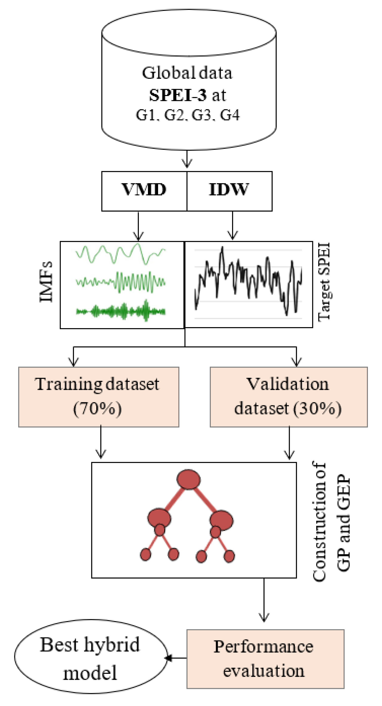
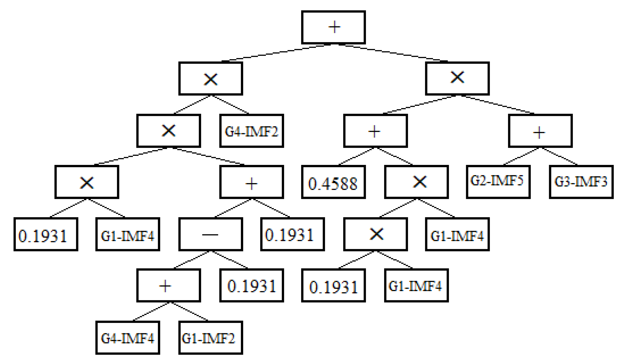
3.4. The Proposed Hybrid VMD-GP Model

As illustrated in Figure 3, the VMD-GP modeling process for automatic prediction of MD at Erbil (i.e., target variable) is commenced by assigning SPEI-3 values to the city, which are calculated with the inverse distance weighting (IDW) interpolation method. In this phase, the closer grid points (i.e., G1 and G2) are more related to the city climate than the farther nodes (i.e., G3 and G4). In the next step, the input variables are created through the VMD. SPEI series, similar to other stochastic time series, contain noises that must be removed to ensure effective model production. These irregular fluctuations in the SPEI series may cause difficulties in model training [47]. Accordingly, GP models could be hybridized with denoising algorithms, which aim to decompose the row SPEI signals (here, SPEI-3 from G1 to G4) for advanced model evolution. To this end, the VMD adaptively separates the grid SPEI series into multiple IMFs that are sorted according to their vibration frequency. Then, a noise reduction filter is applied to the decomposed IMFs, where the rapidly vibrating modes (i.e., the high-frequency components) are removed as redundant IMFs, and hence, will not be contributed to the training process. In this study, the threshold of the noise reduction filter is set to be 20%, for which any vibrating mode with a vibration amplitude less than 20% of the original input signal would be removed as noise. The remaining IMFs were then input into the model for the training and validation process.

Similar to other data-driven models, inputs and corresponding targets are split into training and testing sets. The first 70% of the data were used to train the models to minimize a predefined objective function. Since the GP and GEP engines are trained to predict monthly SPEI with a month lead time (i.e., 1-month ahead forecasts), the target series is shifted one step forward (one may also use one antecedent time-lagged inputs (i.e., t − 1)). The architecture of the VMD-GP models is like its vanilla counterparts (i.e., GP and GEP), except where the input set is substituted with a VMD-denoised input set, which gives a different input shape at a higher dimension.

3.5. Performance Evaluation

To evolve the GP-based models, the root mean squared error (RMSE) was used as the objective function so that during the GP training process, the algorithms attempt to minimize the difference between the actual and predicted SPEI-3 time series. RMSE, together with two other goodness-of-fit measures, namely, Nash–Sutcliffe Efficiency (NSE) and Kling–Gupta Efficiency (KGE), were also adopted to compare the models’ accuracy at both training and validation phases. Like NSE, the KGE equal to 1.0 stands for a perfect agreement between predictions and observations.

$$\mathrm{R}\mathrm{M}\mathrm{S}\mathrm{E}=\sqrt{\frac{\sum _{i=1}^n{{(SPEI}_c-{SPEI}_p)}^2}{n}}$$

(3)

$$\mathrm{N}\mathrm{S}\mathrm{E}=1-\left[\frac{\sum _{i=1}^n{({SPEI}_c-{SPEI}_p)}^2}{\sum _{i=1}^n{({SPEI}_c-\overline{{SPEI}_c})}^2}\right]$$

(4)

$$\mathrm{K}\mathrm{G}\mathrm{E}=1-\sqrt{{\left(CC-1\right)}^2+{(\frac{{\sigma }_p}{{\sigma }_O}-1)}^2+({\frac{\overline{{SPEI}_p}}{\overline{{SPEI}_o}}-1)}^2}$$

(5)

where n denotes the number of data samples used for the training and testing phases. The CC represents the Pearson correlation coefficient. ${SPEI}_O$, ${SPEI}_p$, $\overline{{SPEI}_o}$, and $\overline{{SPEI}_p}$ denote the observed and predicted values of the SPEI-3 and their mean values. The ${\sigma }_O$ and ${\sigma }_p$ stand for the standard deviation of observed and predicted SPEI values, respectively. For additional details on these measures, the reader is referred to [48].

4. Results

4.1. Temporal Variation of SPEI-3 at Erbil

As previously mentioned, the IDW interpolation method with a power of one was used to estimate the temporal variation of SPEI-3 at Erbil using the GDM database demonstrated in Figure 2. Figure 4a depicts the estimated SPEI-3 series based on the distance of the city from the grid points. The figure also illustrated the temporal variation of wet, near normal and dry conditions (i.e., months), separately. The figure shows that the SPEI values vary in the range (−2.5, 2.5) with a slightly negative trend. The near-normal condition (see Figure 4c) is more frequent than both wet (see Figure 4b) and dry (see Figure 4d) conditions. During the past three decades, 40 dry months were estimated, while wet months have occurred 72 times.

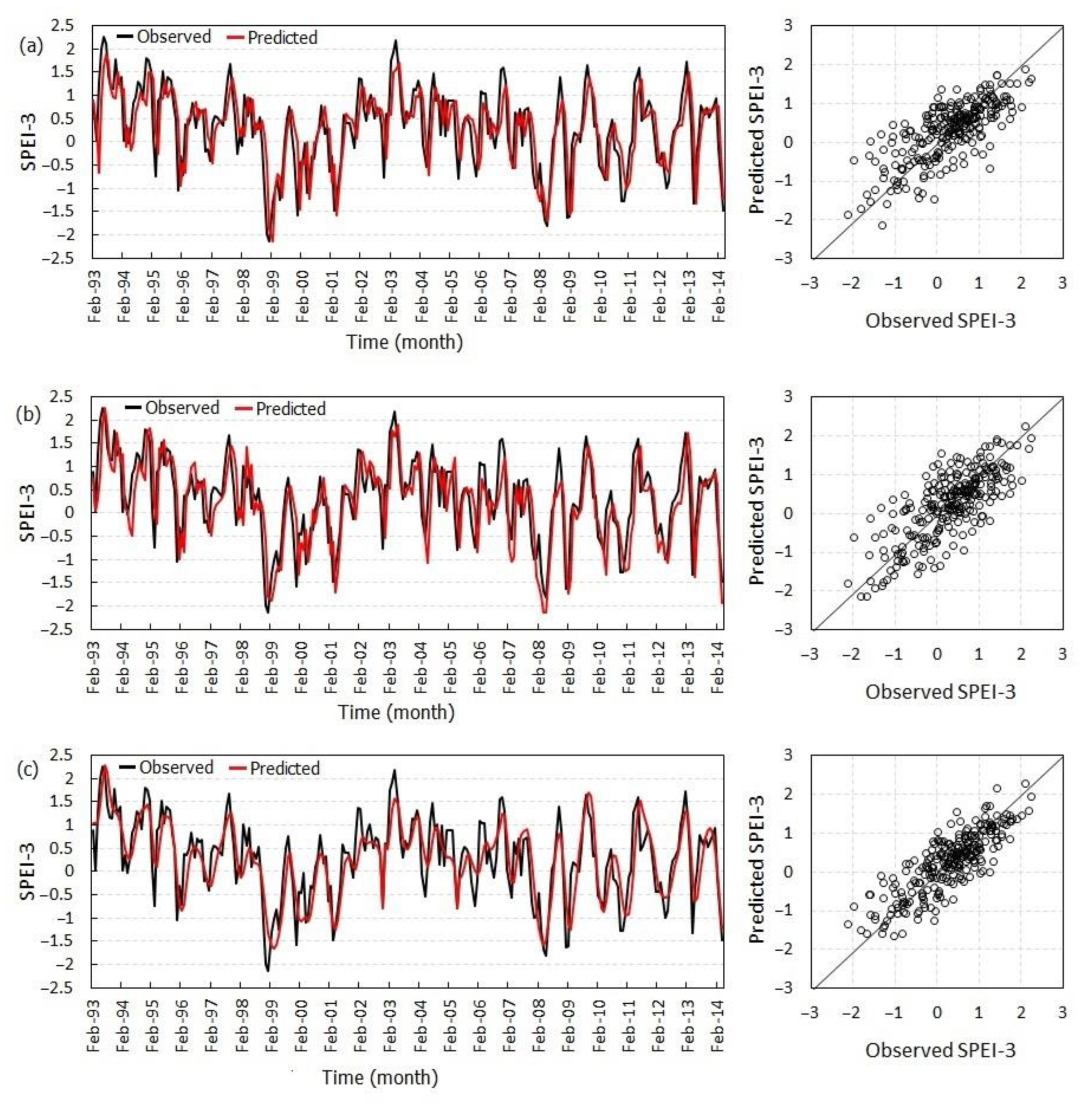
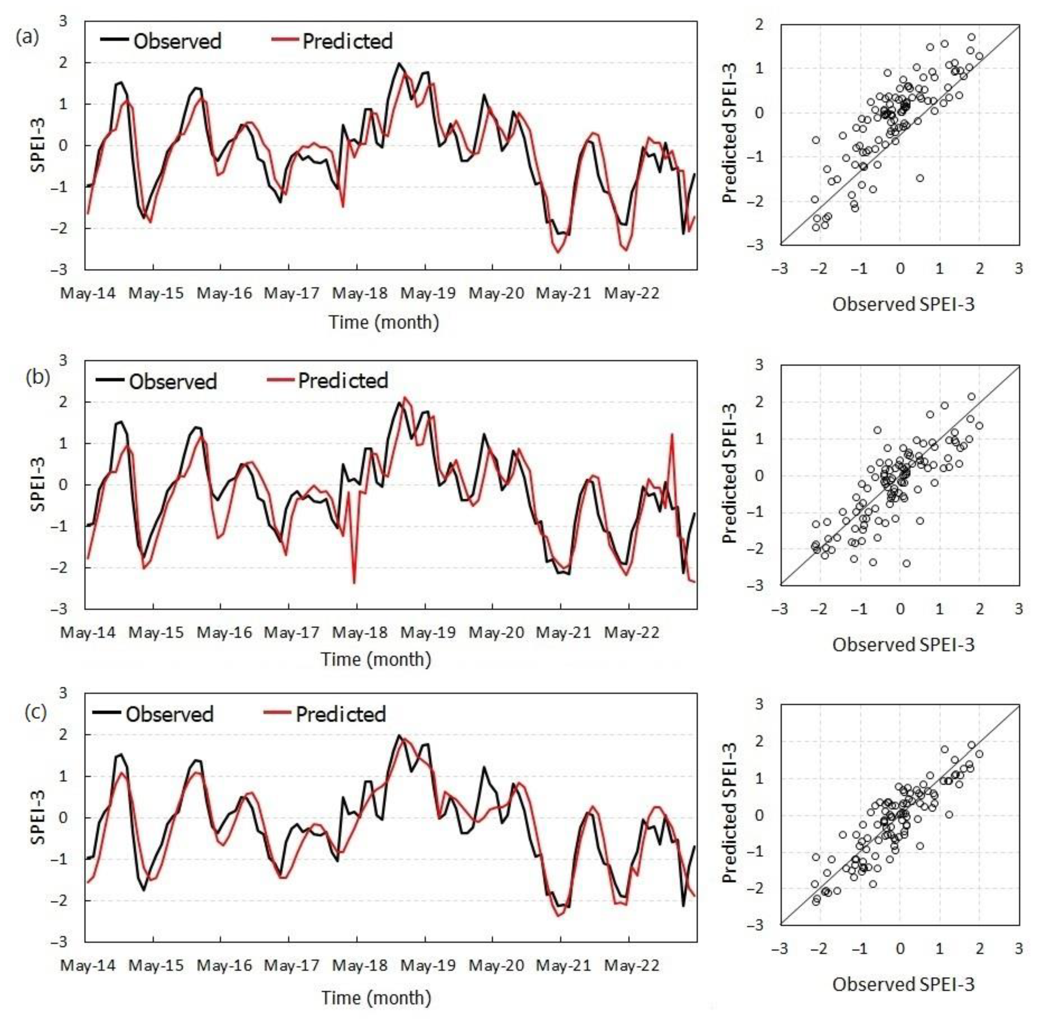
4.2. Benchmark Models

Two standalone benchmarks, namely, GP and GEP, evolved into a month ahead forecast of SPEI-3 at Erbil (Figure 5). The GP and GEP models were built on the GPdotNet [49] and GeneXproTools 5.0 [42] platforms. Given that a single gene expression could hardly extract sufficient underlying features from the stochastic dataset, we designed the GEP models to have at least three expressions (see

Table 2. Parameter setting assigned for GP and GEP training in this study.

Parameter	GP	GEP
Population size	500	500
Mutation Rate	0.1	0.1
Crossover Rate	0.7	0.7
Reproduction rate	0.2	0.2
Maximum genes (trees)	1	3
Maximum number of generations	1000	1000
Max tree depth	7	5
Linking function	NA *	Addition
Tree initialization	Half and Half	Half and Half
Selection method	Rank selection	Rank selection
Function set elements	+, −, ×, ÷, sin, cos, Exp	+, −, ×, ÷, sin, cos, Exp

Note: * NA: Not Applicable.

); however, the depth of each expression was limited to five levels to avoid model complexity and reduce the risk of evolution of overfitted models. The authors’ preliminary runs have demonstrated that GEP models with higher depths not only provide insignificant accuracy improvement, but they may yield risky and overcomplex models. Similarly, for the classic GP setup, the initial number of populations was set to 500 with a maximum depth of 7.0. Our experiments showed that higher values for initial populations for the models with rather a low number of inputs (as is the case in this study) had an insignificant impact on the model performance. The GP and GEP models’ run were terminated after 1000 generations. In addition, an early stopping criterion was used so that the model would stop the training and call back the best model with the lowest validation RMSE when there is no improvement for consecutively 200 iterations. This strategy helps prevent an overfitting scenario due to excessive training. It also helps mitigate an unstable model performance due to insufficient training epochs. Table 2 summarizes the model setup features adopted in this study.

4.3. The Proposed VMD-GP Model

Between the best evolved GP and GEP models, the superb one (here GP) was selected to develop the hybrid VMD-GP to a month ahead forecast of SPEI-3 at Erbil. Given that the VMD decomposition only affects the input set, the VMD-based hybrid model shared the same setup as its standalone counterpart. The VMD algorithm allows the user to adjust the scale number (k) that controls the number of IMFs. Since there is no unified method to determine the optimum scale number [36], we set k = 5.0 in this study. To maintain moderate bandwidth constraint for VMD decomposition, the penalty factor (α) and noise tolerance (τ), respectively, were set to 2000 and 0.0, as suggested by Ali et al. [50]. After 500 iterations, a total of 20 IMF signals with four residual signals were attained for all the nearby grids (i.e., G1, G2, G3, and G4). Figure 6 depicts examples of the IMFs and residual signals attained for the hybrid model generation in the present study.

4.4. Models’ Comparison

Using the obtained IMFs at all nearby grid points, the GP algorithm was trained for the same target variable (i.e., SPEI-3 at Erbil) to attain the VMD-GP model. Similar to GP and GEP runs, the new hybrid models were run to minimize the RMSE as the objective function. To clearly distinguish the accuracy enhancement because of VMD, the same GP setup features were used. Figure 7 shows the best VMD-GP model attained for SPEI-3 prediction at Erbil. The model explicitly combines the most effective IMFs with a set of random numbers generated during the training process. According to the figure, the second and fourth modes of SPEI-3 series at G1 (i.e., G1-IMF2 and G1-IMF4), the fifth mode of G2, the third mode of G3, and the second and fourth modes of SPEI-3 series at G4 are the most influential IMFs for MD prediction at Erbil. These are the best predictors among all 20 IMFs distinguished via the intrinsic input-selecting algorithm of the GP.

Table 3. The performance metrics of the applied predictive models at each station.

	Training			Testing
Models	RMSE	NSE	KGE	RMSE	NSE	KGE
GP	0.586	0.528	0.703	0.549	0.673	0.803
GEP	0.611	0.485	0.620	0.639	0.557	0.113
VMD-GP	0.487	0.674	0.735	0.476	0.754	0.532

listed the performance measures of all the prediction models evolved in this study. The prediction results at both training and testing periods, together with the associated scatterplots, were also depicted in Figure 8 and Figure 9, respectively. Both tabulated and graphical comparisons indicated the superiority of the hybrid model over the standalone models. The minimum RMSE and maximum NSE/KGE in the training phase were attained for the VMD-GP model. Regarding RMSE, NSE, and KGE measures, the achieved accuracy enhancement over the standalone GP is 17%, 28%, and 4.6%, respectively. Considering the testing phase, the hybrid model attained the minimal RMSE and greatest NSE (0.476 and 0.754); however, the GP model has a higher KGE. This indicates that once a model is trained to minimize RMSE, it does not necessarily improve the model in terms of KGE. The table also indicates that the GEP has the lowest accuracy. This is the reason behind the selection of GP to be integrated with VDM. In general, prediction results during the testing period are more accurate than the training phase, which could be due to the narrower range of observed SPEI during the testing period.

Figure 8 and Figure 9 demonstrate that the proposed hybrid model is a robust predictive model capable of capturing the fluctuating trend in the SPEI-3 series based on the nearby grid point IMFs, and, thus, worthy of MD prediction. The scatter plots in the testing period imply that GP (GEP) generally overestimates (underestimates) the observed SPEI. The VMD-GP forecasts are closer to the 1:1 line, indicating their superior accuracy. This can best be justified owing to the elimination of the noise from the predictors that were distilled by VMD.

Inasmuch as the traditional performance measures, such as those used in Table 3, evaluate the hydrological models’ accuracy regarding the mean observed target variable, they might not be efficient indicators for the models’ accuracy once the prediction of extreme events is desired. Thus, it is worth investigating how well the proposed drought prediction model can capture different classes of drought events. To this end, the total number of predicted drought events in the testing period was compared with those observed values in Figure 10. The dry events were compared in three subclasses: moderate (i.e., −1.42 ≤ SPEI ≤ −1.0); severe (i.e., −1.82 ≤ SPEI ≤ −1.43); and extreme (i.e., SPEI ≤ −1.83) events. The figure also illustrates how these events are scattered around the perfect 1:1 line.

This figure shows the occurrence of a total of 19 drought events (eight moderate, four severe, and seven extreme events) during the testing period in the study area. The GP, GEP, and VMD-GP models, respectively, predicted a total of 20, 28, and 25 drought events. Note that these values cannot be interpreted unless their time accuracy is controlled. To this end, Figure 10b was considered to identify the total number of predictions that correspond to observed dry events (SPEI ≤ −1.0). Counting the associated predictions, the figure shows 12, 15, and 16 events for GP, GEP, and VMD-GP. Thus, it can be concluded that the VDM-GP showed the best performance via the prediction of 16 MD events out of 19 observations during the testing period.

5. Discussion

To the best of the authors’ knowledge, no data-driven model for MD forecasting at Erbil has been reported in the literature. On the other hand, there is no unique perfect model for any location as models’ performance may vary according to the frequency domain and discrepancy of the target drought time series. Accordingly, we discussed our model compared with other state-of-the-art models developed for SPEI-3 forecasting at different places. Most of earlier studies reported their models’ performances based on RMSE and NSE; however, RMSE cannot be directly used for models’ comparison due to the scale and range differences between the target SPEI series. Thus, our comparisons were limited to NSE values because it normalizes model performance into an interpretable scale.

The proposed VMD-GP model outperformed several other vanilla and hybrid models available in the literature. For instance, it overcomes the random forest (RF), long short time memory (LSTM), Wavelet Neural Network, and Support Vector Regression models developed by Tian et al. [51] for SPEI-3 prediction in different cities in China. The VMD-GP is also superior to the CNN-LSTM model suggested by Danandeh Mehr et al. [52] for SPEI-3 prediction in two cities in the Ankara province, Turkey. The authors reported the NSE values of their best models equal to 0.49 and 0.53, which are significantly lower than those in this study. Similarly, the VMD-GP model provided more accurate predictions than the RF model optimized by the genetic algorithm developed by Danandeh Mehr et al. [53] for SPEI-3 prediction at Beypazari (NSE = 0.50) and Nallihan (NSE = 0.61) cities in Turkey. Despite the greater performance of the VMD-GP over GP and GEP, our study showed noticeable limitations in attaining an ideal forecast (i.e., NSE > 0.9). This is clearly due to the high stochastic features of drought series that are commonly seen at short time scales SPEI series [54].

6. Conclusions

In this study, we mainly aimed to develop a robust and explicit model for MD prediction in the ungagged catchment. To achieve this goal, we introduced a novel evolutionary technique that implements VMD to decompose GMD datasets into IMFs and a noise signal. The new model, which is called VMD-GP, utilizes GP as the core mapping tool to find the best relationship between the IMFs of the SPEI series of the four closest GMD grid points and the one attained via the IDW method. The results demonstrated that the proposed model provides a prediction accuracy of 0.674 and 0.754 in terms of NSE, respectively, in the training and testing periods. This is equivalent to a 30% and 12% enhancement in the accuracy of the best standalone GP model developed for the study area. It was also found that, at most, two modes of the grided SPEI-3 signals effectively impacted the subsequent SPEI-3 in our study area. The intrinsic input selection algorithm of GP was able to identify the redundant IMFs and remove them from the final solution.

All in all, the results revealed that the proposed VMD-GP model is a promising solution for the month ahead MD prediction in Erbil, which suffers from scarce meteorological observations. The proposed model is explicit, and thus, it could be useful for the proper planning and efficient watershed management in the study area. A similar methodology can be adopted for MD prediction at any ungagged catchments. Relying on the intrinsic input selection feature of GP, a predefined scale number, i.e., a total of five IMFs, was adopted in this study. The optimum number of IMFs and the ideal noise reduction threshold could be investigated in future studies that might yield more accurate forecasts. To this end, optimization algorithms based on some metaheuristic methods (evolutionary algorithms, physics-based algorithms, swarm intelligence) could be implemented.

References

1. Li, J.; Wang, Z.; Wu, X.; Xu, C.; Guo, S.; Chen, X. Toward Monitoring Short-Term Droughts Using a Novel Daily Scale, Standardized Antecedent Precipitation Evapotranspiration Index. J. Hydrometeorol. 2020, 21, 891–908. [Google Scholar] [CrossRef] [Green Version]
2. Li, J.; Wang, Z.; Wu, X.; Zscheischler, J.; Guo, S.; Chen, X.A. Standardized index for assessing sub-monthly compound dry and hot conditions with application in China. Hydrol. Earth Syst. Sci. 2021, 25, 1587–1601. [Google Scholar] [CrossRef]
3. Piao, S.; Ciais, P.; Huang, Y.; Shen, Z.; Peng, S.; Li, J.; Zhou, L.; Liu, H.; Ma, Y.; Ding, Y.; et al. The Impacts of Climate Change on Water Resources and Agriculture in China. Nature 2010, 467, 43–51. [Google Scholar] [CrossRef] [PubMed]
4. Zhu, G.; Liu, Y.; Wang, L.; Sang, L.; Zhao, K.; Zhang, Z.; Qiu, D. The isotopes of precipitation have climate change signal in arid Central Asia. Glob. Planet. Chang. 2023, 225, 104103. [Google Scholar] [CrossRef]
5. Yue, Z.; Zhou, W.; Li, T. Impact of the Indian Ocean Dipole on Evolution of the Subsequent ENSO: Relative Roles of Dynamic and Thermodynamic Processes. J. Clim. 2021, 34, 3591–3607. [Google Scholar] [CrossRef]
6. Mann, M.E.; Lloyd, E.A.; Oreskes, N. Assessing Climate Change Impacts on Extreme Weather Events: The Case for an Alternative (Bayesian) Approach. Clim. Chang. 2017, 144, 131–142. [Google Scholar] [CrossRef]
7. Gao, C.; Zhang, B.; Shao, S.; Hao, M.; Zhang, Y.; Xu, Y.; Wang, Z. Risk assessment and zoning of flood disaster in Wuchengxiyu Region, China. Urban Clim. 2023, 49, 101562. [Google Scholar] [CrossRef]
8. Zhu, X.; Xu, Z.; Liu, Z.; Liu, M.; Yin, Z.; Yin, L.; Zheng, W. Impact of dam construction on precipitation: A regional perspective. Mar. Freshw. Res. 2022, 74, 877–890. [Google Scholar] [CrossRef]
9. Zhou, J.; Wang, L.; Zhong, X.; Yao, T.; Qi, J.; Wang, Y.; Xue, Y. Quantifying the major drivers for the expanding lakes in the interior Tibetan Plateau. Sci. Bull. 2022, 67, 474–478. [Google Scholar] [CrossRef]
10. Pei, Y.; Qiu, H.; Zhu, Y.; Wang, J.; Yang, D.; Tang, B.; Cao, M. Elevation dependence of landslide activity induced by climate change in the eastern Pamirs. Landslides 2023, 20, 1115–1133. [Google Scholar] [CrossRef]
11. Bedri, R.; Piechota, T. Future Colorado River Basin Drought and Surplus. Hydrology 2022, 9, 227. [Google Scholar] [CrossRef]
12. Woolway, R.I.; Kraemer, B.M.; Lenters, J.D.; Merchant, C.J.; O’Reilly, C.M.; Sharma, S. Global Lake Responses to Climate Change. Nat. Rev. Earth Environ. 2020, 1, 388–403. [Google Scholar] [CrossRef]
13. Maghrebi, M.; Noori, R.; Mehr, A.D.; Lak, R.; Darougheh, F.; Razmgir, R.; Kløve, B. Spatiotemporal changes in Iranian rivers’ discharge. Elem. Sci. Anth. 2023, 11, 00002. [Google Scholar] [CrossRef]
14. Wambura, F.J.; Dietrich, O. Analysis of Agricultural Drought Using Remotely Sensed Evapotranspiration in a Data-Scarce Catchment. Water 2020, 12, 998. [Google Scholar] [CrossRef] [Green Version]
15. Danandeh Mehr, A.; Vaheddoost, B.; Mohammadi, B. ENN-SA: A Novel Neuro-Annealing Model for Multi-Station Drought Prediction. Comput. Geosci. 2020, 145, 104622. [Google Scholar] [CrossRef]
16. Tian, H.; Huang, N.; Niu, Z.; Qin, Y.; Pei, J.; Wang, J. Mapping Winter Crops in China with Multi-Source Satellite Imagery and Phenology-Based Algorithm. Remote Sens. 2019, 11, 820. [Google Scholar] [CrossRef] [Green Version]
17. Liu, Z.; Xu, J.; Liu, M.; Yin, Z.; Liu, X.; Yin, L.; Zheng, W. Remote sensing and geostatistics in urban water-resource monitoring: A review. Mar. Freshw. Res. 2023. [Google Scholar] [CrossRef]
18. McClean, F.; Dawson, R.; Kilsby, C. Intercomparison of Global Reanalysis Precipitation for Flood Risk Modelling. Hydrol. Earth Syst. Sci. 2023, 27, 331–347. [Google Scholar] [CrossRef]
19. Vicente-Serrano, S.M.; Beguería, S.; López-Moreno, J.I. A Multiscalar Drought Index Sensitive to Global Warming: The Standardized Precipitation Evapotranspiration Index. J. Clim. 2010, 23, 1696–1718. [Google Scholar] [CrossRef] [Green Version]
20. Xu, H.; Xu, C.Y.; Chen, S.; Chen, H. Similarity and Difference of Global Reanalysis Datasets (WFD and APHRODITE) in Driving Lumped and Distributed Hydrological Models in a Humid Region of China. J. Hydrol. 2016, 542, 343–356. [Google Scholar] [CrossRef]
21. Seyyedi, H.; Anagnostou, E.N.; Beighley, E.; McCollum, J. Hydrologic Evaluation of Satellite and Reanalysis Precipitation Datasets over a Mid-Latitude Basin. Atmos. Res. 2015, 164–165, 37–48. [Google Scholar] [CrossRef]
22. Zhang, R.; Li, L.; Zhang, Y.; Huang, F.; Li, J.; Liu, W.; Mao, T.; Xiong, Z.; Shangguan, W. Assessment of Agricultural Drought Using Soil Water Deficit Index Based on ERA5-Land Soil Moisture Data in Four Southern Provinces of China. Agriculture 2021, 11, 411. [Google Scholar] [CrossRef]
23. Rakhmatova, N.; Arushanov, M.; Shardakova, L.; Nishonov, B.; Taryannikova, R.; Rakhmatova, V.; Belikov, D.A. Evaluation of the Perspective of ERA-Interim and ERA5 Reanalyses for Calculation of Drought Indicators for Uzbekistan. Atmosphere 2021, 12, 527. [Google Scholar] [CrossRef]
24. Vicente-Serrano, S.M.; Domínguez-Castro, F.; Reig, F.; Tomas-Burguera, M.; Peña-Angulo, D.; Latorre, B.; El Kenawy, A. A global drought monitoring system and dataset based on ERA5 reanalysis: A focus on crop-growing regions. Geosci. Data J. 2022. [Google Scholar] [CrossRef]
25. Mustafa Alee, M.; Danandeh Mehr, A.; Akdegirmen, O.; Nourani, V. Drought Assessment across Erbil Using Satellite Products. Sustainability 2023, 15, 6687. [Google Scholar] [CrossRef]
26. Hameed, M.; Ahmadalipour, A.; Moradkhani, H. Apprehensive Drought Characteristics over Iraq: Results of a Multidecadal Spatiotemporal Assessment. Geosciences 2018, 8, 58. [Google Scholar] [CrossRef] [Green Version]
27. Jasim, A.I.; Awchi, T.A. Regional Meteorological Drought Assessment in Iraq. Arab. J. Geosci. 2020, 13, 284. [Google Scholar] [CrossRef]
28. Hussein, S.O.; Kovács, F.; Tobak, Z. Spatiotemporal Assessment of Vegetation Indices Aand Land Cover for Erbil City And Its Surrounding Using Modis Imageries. J. Environ. Geogr. 2017, 10, 31–39. [Google Scholar] [CrossRef] [Green Version]
29. Suliman, A.H.A.; Awchi, T.A.; Al-Mola, M.; Shahid, S. Evaluation of Remotely Sensed Precipitation Sources for Drought Assessment in Semi-Arid Iraq. Atmos. Res. 2020, 242, 105007. [Google Scholar] [CrossRef]
30. Al-Timimi, Y.K.; George, L.E.; Al-Jiboori, M.H. Drought Risk Assessment in Iraq Using Remote Sensing And GIS Techniques. Iraqi J. Sci. 2012, 53, 1078–1082. [Google Scholar]
31. Almamalachy, Y.S.; Al-Quraishi, A.M.F.; Moradkhani, H. Agricultural Drought Monitoring Over Iraq Utilizing MODIS Products. Environ. Remote Sens. GIS Iraq 2020, 253–278. [Google Scholar] [CrossRef]
32. Al-Juboori, A.M. Prediction of Hydrological Drought in Semi-Arid Regions Using a Novel Hybrid Model. Water Resour. Manag. 2023, 37, 3657–3669. [Google Scholar] [CrossRef]
33. Danandeh Mehr, A.; Tur, R.; Çalışkan, C.; Tas, E. A Novel Fuzzy Random Forest Model for Meteorological Drought Classification and Prediction in Ungauged Catchments. Pure Appl. Geophys. 2020, 177, 5993–6006. [Google Scholar] [CrossRef]
34. Mehr, A.D.; Sorman, A.U.; Kahya, E.; Afshar, M. Climate Change Impacts on Meteorological Drought Using SPI and SPEI: Case Study of Ankara, Turkey. Hydrol. Sci. J. 2019, 65, 254–268. [Google Scholar] [CrossRef]
35. Dragomiretskiy, K.; Zosso, D. Variational Mode Decomposition. IEEE Trans. Signal Process. 2014, 62, 531–544. [Google Scholar] [CrossRef]
36. Wu, S.; Feng, F.; Zhu, J.; Wu, C.; Zhang, G. A Method for Determining Intrinsic Mode Function Number in Variational Mode Decomposition and Its Application to Bearing Vibration Signal Processing. Shock. Vib. 2020, 8304903. [Google Scholar] [CrossRef]
37. Huang, Y.; Lin, J.; Liu, Z.; Wu, W. A Modified Scale-Space Guiding Variational Mode Decomposition for High-Speed Railway Bearing Fault Diagnosis. J. Sound Vib. 2019, 444, 216–234. [Google Scholar] [CrossRef]
38. Maji, U.; Pal, S. Empirical Mode Decomposition vs. Variational Mode Decomposition on ECG Signal Processing: A Comparative Study. In Proceedings of the 2016 International Conference on Advances in Computing, Communications and Informatics ICACCI, Jaipur, India, 21–24 September 2016; pp. 1129–1134. [Google Scholar] [CrossRef]
39. Koza, J.R. Genetic Programming as a Means for Programming Computers by Natural Selection. Stat. Comput. 1994, 4, 87–112. [Google Scholar] [CrossRef]
40. Babovic, V.; Keijzer, M. Genetic Programming as a Model Induction Engine. J. Hydroinform. 2000, 2, 35–60. [Google Scholar] [CrossRef] [Green Version]
41. Kisi, O.; Dailr, A.H.; Cimen, M.; Shiri, J. Suspended Sediment Modeling Using Genetic Programming and Soft Computing Techniques. J. Hydrol. 2012, 450–451, 48–58. [Google Scholar] [CrossRef]
42. Ferreira, C. Gene Expression Programming: Mathematical Modeling by an Artificial Intelligence; Springer: Berlin/Heidelberg, Germany, 2006; Volume 21. [Google Scholar]
43. Searson, D.P. GPTIPS 2: An Open-Source Software Platform for Symbolic Data Mining. In Handbook of Genetic Programming Applications; Springer International Publishing: Cham, Switzerland, 2015; pp. 551–573. [Google Scholar] [CrossRef] [Green Version]
44. Brameier, M.; Banzhaf, W.; Banzhaf, W. Linear Genetic Programming; Springer: New York, NY, USA, 2007. [Google Scholar] [CrossRef]
45. Gandomi, A.H.; Alavi, A.H. Multi-Stage Genetic Programming: A New Strategy to Nonlinear System Modeling. Inf. Sci. 2011, 181, 5227–5239. [Google Scholar] [CrossRef]
46. Mohammad-Azari, S.; Bozorg-Haddad, O.; Loáiciga, H.A. State-of-Art of Genetic Programming Applications in Water-Resources Systems Analysis. Environ. Monit. Assess 2020, 192, 73. [Google Scholar] [CrossRef] [PubMed]
47. Azzali, I.; Vanneschi, L.; Bakurov, I.; Silva, S.; Ivaldi, M.; Giacobini, M. Towards the Use of Vector Based GP to Predict Physiological Time Series. Appl. Soft Comput. 2020, 89, 106097. [Google Scholar] [CrossRef] [Green Version]
48. Althoff, D.; Rodrigues, L.N. Goodness-of-fit criteria for hydrological models: Model calibration and performance assessment. J. Hydrol. 2021, 600, 126674. [Google Scholar] [CrossRef]
49. Hrnjica, B.; Danandeh Mehr, A. Optimized Genetic Programming Applications; IGI Global: Hershey, PA, USA, 2018; p. 310. [Google Scholar] [CrossRef]
50. Ali, M.; Prasad, R.; Xiang, Y.; Khan, M.; Ahsan Farooque, A.; Zong, T.; Yaseen, Z.M. Variational Mode Decomposition Based Random Forest Model for Solar Radiation Forecasting: New Emerging Machine Learning Technology. Energy Rep. 2021, 7, 6700–6717. [Google Scholar] [CrossRef]
51. Tian, W.; Wu, J.; Cui, H.; Hu, T. Drought prediction based on feature-based transfer learning and time series imaging. IEEE Access 2021, 9, 101454–101468. [Google Scholar] [CrossRef]
52. Danandeh Mehr, A.; Rikhtehgar Ghiasi, A.; Yaseen, Z.M.; Sorman, A.U.; Abualigah, L. A Novel Intelligent Deep Learning Predictive Model for Meteorological Drought Forecasting. J. Ambient. Intell. Humaniz. Comput. 2023, 14, 10441–10455. [Google Scholar] [CrossRef]
53. Danandeh Mehr, A.; Torabi Haghighi, A.; Jabarnejad, M.; Safari, M.J.S.; Nourani, V. A New Evolutionary Hybrid Random Forest Model for SPEI Forecasting. Water 2022, 14, 755. [Google Scholar] [CrossRef]
54. Gholizadeh, R.; Yılmaz, H.; Danandeh Mehr, A. Multitemporal Meteorological Drought Forecasting Using Bat-ELM. Acta Geophys. 2022, 70, 917–927. [Google Scholar] [CrossRef]
Figure 1. Location of drought for global SPEI grid points closest to Erbil, Iraq.
Water 15 02686 g001
Figure 2. The SPEI-3 time series at global drought monitoring grid points closest to Erbil.
Water 15 02686 g002
Figure 3. Schematic view of the proposed VMD-GP model.
Water 15 02686 g003
Figure 4. The (a) SPEI-3 time series at Erbil estimated by IDW interpolation together with distribution of (b) wet, (c) near normal, and (d) dry months.
Water 15 02686 g004
Figure 5. The best vanilla (a) GP and (b) GEP models evolved for SPEI-3 prediction at Erbil.
Water 15 02686 g005
Figure 6. Examples of IMFs and residuals of the global SPEI-3 time series at G1 (left panel) and G4 (right panel) obtained by applying VMD.
Water 15 02686 g006
Figure 7. The best evolved VMD-GP model for month ahead SPEI-3 forecasting at Erbil, Iraq.
Water 15 02686 g007
Figure 8. Time series and scatter plot presentations of the observed and predicted SPEI-3 during the training period; (a) GP, (b) GEP, and (c) VMD-GP models.
Water 15 02686 g008
Figure 9. Time series and scatter plot presentations of the observed and predicted SPEI-3 during the testing period; (a) GP, (b) GEP, and (c) VMD-GP models.
Water 15 02686 g009
Figure 10. Number of observed and predicted droughts (a) and their scatter plot (b).
Water 15 02686 g010