Article

Characteristic Analysis and Uncertainty Assessment of the Joint Distribution of Runoff and Sediment: A Case Study of the Huangfuchuan River Basin, China

College of Water Resources, North China University of Water Resources and Electric Power, Zhengzhou 450045, China
*
Author to whom correspondence should be addressed.
Water 2023, 15(14), 2644; https://doi.org/10.3390/w15142644
Submission received: 18 June 2023 / Revised: 13 July 2023 / Accepted: 17 July 2023 / Published: 20 July 2023

Abstract

:
Exploring the relationship between runoff and sediment elements in a river basin is a prerequisite for realizing the scientific management scheme of runoff and sediment. In this study, six commonly applied probability distributions are utilized to fit the marginal distribution, and three Archimedes copulas are used to fit the joint distribution to build a joint probability distribution model of river runoff and sediment in sandy areas. The synchronous and asynchronous encounter probabilities of runoff and sediment are calculated. The uncertainties of marginal distribution, parameter estimation, and copula function in the process of constructing the joint distribution model framework are analyzed. The results indicate that: (1) The runoff and sediment series from 1954 to 2015 of the Huangfuchuan River basin are divided into three stages by using the cumulative anomaly method and the double mass curve method, and the runoff and sediment in the three stages have strong correlations. In the  T a  (1954–1978) and  T b  (1979–1996) stages, the optimal joint distribution functions of runoff and sediment are Gumbel, and in the  T c  (1997–2015) stage the optimal joint distribution function is Clayton; (2) The synchronous probabilities of runoff and sediment series in the three stages are 69.84%, 84.82%, and 70.72%, respectively, which are much greater than the asynchronous frequencies of abundance and depletion, and this showed that the conditions of runoff and sediment in the river basin are consistent; (3) The joint distribution function is sensitive to the choice of marginal distributions, parameters, and copula functions, and the optimal marginal distribution function, optimal copula function, and the parameters selected by the maximum likelihood estimation method can better fit the runoff-sediment relationship in the river basin and reduce the process uncertainty.

1. Introduction

The interdependence and response processes of runoff and sediment elements in river basins have always been the focus of water science research [1,2,3]. Runoff and sediment are carriers of material transport in river systems and outputs of runoff and sediment production processes in river basins [4,5,6]; their relationship and synergistic evolution play an irreplaceable role in the function of watershed systems [7]. The research of the joint probability of runoff and sediment is a prerequisite for realizing the scientific management scheme of runoff and sediment, which is of great importance in the utilization of water resources, sustainable development of the river basin, flood control, soil and water conservation, and ecological construction [8,9,10,11].
Hydrological events are complex stochastic events coupled with multiple factors, and correlations commonly exist among their internal variables. The use of traditional univariate hydrological frequency analysis is difficult to fully reflect the dependencies among the variables of hydrological events and has limitations [12,13,14]. Traditional multivariate hydrological analysis calculations also mainly tend to adopt linear correlation multivariate distribution models with the same marginal distribution [15,16], limiting the accuracy of their results. Copula function is a breakthrough method for establishing multivariate joint distributions [17], which can connect two or more correlated variables [18] and study the marginal distribution and correlation structure, respectively, without restricting the type of marginal distributions. It has high adaptability and is widely used in hydrological and water resources application fields, such as frequency analysis, risk analysis, stochastic simulation of rainfall, floods, droughts, etc. [19,20,21,22,23] Golian et al. employed the copula method to study the joint probability distribution of rainfall depth and peak flow [24]; Bacchi and Balistrocchi proposed a criterion for deriving flood frequency curves from rainfall and duration distribution, and evaluated the return period of bivariate rainfall events [25]; Zhang et al. utilized copula functions to focus on the relationship between groundwater depth changes and three selected control factors from a probability perspective, and compared the differences between the results of the two-dimensional and three-dimensional copula functions [18]; Requena et al. applied the copula approach to perform multivariate flood frequency analyses, and the uncertainty involved in selecting copula to characterize the dependency structure of short data sequences is analyzed [26]; Chang et al. constructed a two-dimensional copula drought risk model of drought duration and severity, and the drought risk of Weihe River Basin was fully assessed [27]; Li et al. constructed a model of runoff and sediment over two stations in the Anning watershed 2010~2015 using the copula analysis method, analyzing the synchronous and asynchronous probabilities of runoff and sediment from both time and space perspectives [28]; Dodangeh et al. established a joint probabilistic model of the extreme rainfall–runoff, using annual maximum precipitation, corresponding historical and simulated runoff data [29]; Salvadori et al. introduced a framework for multivariate copula for handing multivariate disaster scenarios and evaluated the threat probability of natural disasters [30].
Due to its complex physical mechanisms and numerous influencing factors (including climate, meteorology, topography, geomorphology, underlying surface, etc.,), uncertainties in hydrological processes are prevalent, and the degree of uncertainty is directly related to the complexity of the system [31]. Uncertainties in the framework of multidimensional variable models based on copula theory include the uncertainty in the marginal distribution, the uncertainty in the selection of copula functions, and the uncertainties in sample sampling and parameter estimation [32,33]. The uncertainty in the process of constructing the copula joint distribution model has a significant impact on the accuracy of the conclusion and the correctness of the decision. Comprehensive assessment of uncertainty in joint distribution models has complexity, and the quantitative analysis of uncertainty has rarely been addressed in previous studies, and related research is currently at the initial stage.
The Yellow River has the highest sediment concentration in the world and is the world’s most famous sandy river. In recent years, under the combined influence of climate change and human activities, the runoff–sediment process of the Yellow River has changed significantly [34]. The Huangfuchuan River basin is a typical basin in the concentrated source area of sandy and coarse sediment in the middle reaches of the Yellow River (Heilong interval), which is one of the main production areas of coarse sediment in the Yellow River and the basin with the highest erosion intensity among the tributaries of the Yellow River. Since the 20th century, due to the over-exploitation of coal resources in the Huangfuchuan River basin, the groundwater level has continued to decline, runoff has shown a decreasing trend, and droughts have continued to occur in the arid zone. In addition, arsenic sandstone has been exposed in a large area in the basin, and the original vegetation has been severely damaged. These features are extremely rare in China and even around the world. Under the changing environment, the modeling and analysis of the synergistic evolution of runoff and sediment in the Huangfuchuan River basin can help clarify the runoff-sediment relationship and the change patterns in the Yellow River basin and help guide watershed management planning and soil erosion control. It is the theoretical basis for establishing a runoff-sediment regulation system for the harmonious development of man and nature. It provides the scientific basis and data support for runoff-sediment resource utilization in the region, is theoretical support for the formulation of regional sustainable development countermeasures, and is of practical significance for the ecological environment construction of the Loess Plateau, the healthy management of the Yellow River, and the high-quality development of the Yellow River basin.
In this paper, the Huangfuchuan River basin is taken as the research object, the joint probability distribution model of runoff and sediment in a sandy area is constructed, and the uncertainties in the process of constructing the copula joint distribution function are analyzed. Firstly, the cumulative anomaly method, the double mass curve (DMC) method, and the Mann-Kendall test are used to analyze the runoff and sediment discharge series from 1954 to 2015, determine the mutation points, and divide them into three stages; the copula function is introduced to construct the joint distribution model of runoff and sediment in each stage, calculate the synchronous and asynchronous encounter probabilities of runoff and sediment, and analyze the joint return period and the co-occurrence return period. Finally, the uncertainties of the marginal distribution, parameters estimation, and the copula function are analyzed.

2. Materials and Methods

2.1. Study Area and Data Sources

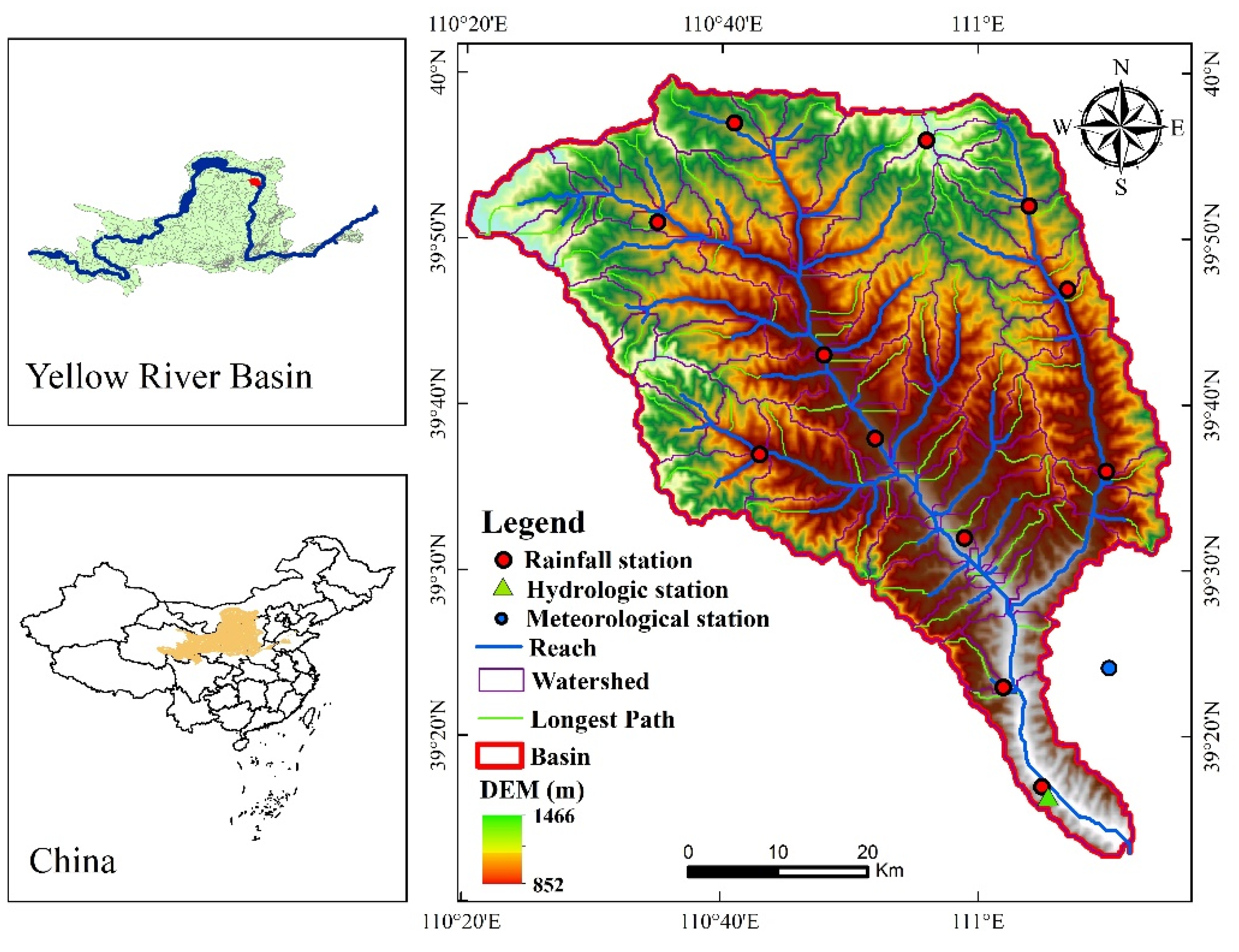
Huangfuchuan is located on the upper right bank of the middle reaches of the Yellow River between Hekou town and the Longmen area. It is a first-class tributary of the Yellow River, which originates in the eastern part of the Ordos Plateau, the transition zone between the Loess Plateau and the desert grassland, flowing through the Jungar Banner of Inner Mongolia Autonomous Region, and flows into the Yellow River in Fugu County, Shanxi Province. As shown in Figure 1, the mainstream has a length of 137 km and a basin area of 3246 km2. The basin is located inland, influenced by the southeast monsoon, and has a continental monsoon climate with an average precipitation of 350–450 mm per year, and the distribution is extremely uneven during the year, with more than 80% of annual precipitation concentrated in June to September. Huangfuchuan belongs to a sandy and coarse sediment river, with an average annual sediment discharge of 61.2 million tons and an average annual sediment modulus of 19.1 million tons/(km2·a), which is one of the most serious zones of soil erosion in the Loess Plateau area and transports a large amount of coarse sediment to the Yellow River. The Huangfuchuan hydrologic station is close to the basin outlet, controlling a basin area of 3199 km2. The main tasks of the station include precipitation, water level, flow, sediment testing, etc. It is a national basic hydrological station.
The hydrological data used in this study were from the Yellow River Conservancy Commission of the Ministry of Water Resources and the Yellow River Basin Hydrological Yearbook, and the measured runoff and sediment data from 1954 to 2015 were selected from Huangfuchuan Hydrological Station, the outlet station of Huangfuchuan River basin. We collected data from 12 rainfall stations in the Huangfuchuan River basin and used the interpolation method of selecting neighboring stations to interpolate the missing data. The Thiessen polygons module of Arcgis 10.3 software was used to obtain basin surface precipitation data.

2.2. Mutation Analysis

2.2.1. The Cumulative Anomaly Method

The cumulative anomaly method is basic and widely used in mutation detection [35,36]. This method cumulates the departure value between each datum and the average of the time series, and according to the change of cumulative value slope and extreme points, the mutation point is detected to judge the time of time series mutation. For the time series  X i X 1 , X 2 , , X n , cumulative anomalies  C t  can be expressed as:
C t = i = 1 t ( X i X ¯ ) ( t = 1 , 2 , 3 , , n )
where  X i  is the discrete values of the data series, and  X ¯  is the average of the data series.

2.2.2. The Double Mass Curve Method

The double mass curve (DMC) method is a method based on linear regression assessment to investigate long-term trends and detect change points of hydro-meteorological time series [37]. The basic principle of this method is to accumulate the two variables under investigation step by step for the same length of time, take the two accumulated values as horizontal and vertical coordinates, respectively, and observe the change in slope. If the ratio between the two variables remains constant, the relationship is linear over the same time. Conversely, it indicates that the original relationship between the two variables has changed. The time corresponding to the point where the slope of the straight line deviates significantly is the year when the variable begins to undergo significant changes. Namely:
S = a R + b
where S and R denote sediment discharge and runoff, respectively, and a and b are coefficients.

2.3. Trend Analysis

2.3.1. The M-K Trend Test

The Mann-Kendall trend test [38,39] is a non-parametric test method that does not require samples to follow a certain distribution. It is often used for analyzing the trend of time series changes in hydrological and meteorological elements. In the M-K test, the calculation formula for the test statistic S is:
S = i = 1 n 1 j = i + 1 n sgn X j X i
where n is the length of the time series, and  X i  and  X j  represent the values at the  i th  and  j th  time points, respectively  j > i . Among them:
sgn X j X i = + 1 i f   X j X i > 0 0 i f   X j X i = 0 1 i f   X j X i < 0
V a r S = 1 18 n n 1 2 n + 5 p = 1 q t p t p 1 2 t p + 5
where q is the number of the tied values, and  t p  is the number of ties for the  p th  value.
The calculation formula for Mann-Kendall trend test statistics is:
Z S _ M K = S 1 V a r S i f   S > 0 0 i f   S = 0 S + 1 V a r S i f   S = 0
In a two-tailed test, if  Z s _ M K Z 1 α / 2 , this indicates a significant trend in the sequence at significance level  α .

2.3.2. The TFPW—MK Test

In trend analysis, in order to eliminate serial autocorrelation, it is usually necessary to perform pre-whitening processing. The Mann-Kendall test with trend-free pre-whitening (TFPW-MK) [40] is a pre-whitening treatment based on M-K, which effectively reduces the influence of series autocorrelation and ensures the accuracy of the test. The operation steps are as follows:
(1)
Construct the trend-free series Yt:
Y t = X t β t
where  X t  is the series value at the year t, and  β  is the trend slope.
(2)
Calculate the first-order autocorrelation coefficient of the series Yt, and perform a significance test. When  r 1  is not significant, a detrended series is used for trend detection. On the contrary, the detrended series is pre-whitened, and the residual series is recorded as  Z t .
r 1 = 1 n 1 i = 1 n 1 x i E x i x i + 1 E x i 1 n i = 1 n x i E x i 2
Z t = Y t r 1 Y t 1
(3)
The residual sequence is reorganized with the trend term to form a trend-free pre-whitening series  X t * :
X t = Z t β t .
(4)
Perform an M-K trend test on series  X t * .

2.4. Marginal Distribution Model

Normal (NOR), gamma (GAM), exponential (EXP), Weibull (WBL), generalized extreme value (GEV), and log-normal (LOGN) are the commonly used types of probability distributions. The above six univariate distribution functions are selected to fit the runoff and sediment discharge of Huangfuchuan hydrologic station as their marginal distribution functions. The maximum likelihood method is used to estimate the parameters, and the Kolmogorov-Smirnov (K-S) test is used to test whether the samples obeyed a certain marginal function, and the principle of the minimum deviation square (OLS) and Akaike information criterion (AIC) [41] are used to evaluate the goodness-of-fit of the marginal function.
(1) Kolmogorov-Smirnov (K-S) Test: The K-S test is a test based on the cumulative distribution function to test whether two empirical distributions or an empirical distribution and a theoretical distribution are different. The hypothesis test problem is that the overall sample obeys a particular distribution (H0) and the overall sample distribution does not obey a particular distribution (H1).
(2) Ordinary least square (OLS): The OLS is the minimum deviation square criterion. The OLS is used to measure the deviation between the theoretical and empirical values, and the smaller the value the better the curve fit, which is calculated as follows:
O L S = 1 n i = 1 n P e i P i 2
where  p i  and  p e i  are theoretical and empirical frequencies, respectively.
(3) Akaike information criterion (AIC): AIC is one of the criteria used to evaluate the merit of the model. The smaller the AIC value, the better the curve fit, and its formula is as follows:
A I C = n ln ( M S E ) + 2 m
M S E = 1 n m i = 1 n p e i p i 2
where MSE is the root-mean-square deviation, n is the sample size, and m is the number of model parameters.

2.5. Copula Joint Distribution Model

The copula function was proposed by Sklar in 1959 [42]. It is a multi-dimensional function defined on the interval [0, 1], connecting the joint distribution and the respective marginal distribution.
Sklar’s theorem is the theoretical basis of the copula function. For two random variables X and Y, there are two-dimensional joint distribution functions  F X , Y x , y , and the marginal distribution functions of the variables X and Y are    R X x  and  S Y y , respectively. Then there exists a copula function C, such that:
F X , Y x , y = C R X x , S Y y C ( u , v )
If the marginal distribution functions  R X x  and  S Y y  are continuous functions, the copula function C is unique.
There are many classifications of copula functions, among which Archimedean copulas are widely used in the field of hydrology because of their simple form and strong adaptability. In this paper, the three most commonly used two-dimensional Archimedean copula functions are selected to construct the two-dimensional joint distribution, and their cumulative distribution functions are shown in Table 1. The parameters θ of Copula functions are estimated by the maximum likelihood estimation method, and the OLS criterion, AIC information criterion, and Bayesian information criterion are used for testing the goodness of fit to determine the optimal copula functions.
Bayesian information criterion (BIC):
B I C = n ln M S E + m ln n
where n is the sample size, and m is the number of model parameters. The smaller the BIC value, the better the fitting effect.

2.6. Runoff-Sediment Encounter Probability Analysis

Using pf = 37.5% and pk = 62.5% as the frequency criteria for the division of runoff and sediment rich or poor status, respectively, the hydrological probability method is used to divide the rich-poor of runoff and sediment, and the encounter combination between the two can be divided into the following nine scenarios shown in Table 2.

2.7. Return Period Analysis

The return period refers to the average recurrence interval between the occurrences of an observation greater than or equal to 1 time during the statistical period of the data. The return period is an important indicator in water engineering. There are two cases of binary return period: one is called the joint return period, which means the return period when the design value of either of the two variables is exceeded ( X x    or  Y y ), and here it is expressed by  T o r ; the second is called the co-occurrence return period, which means the return period when the design values of two variables are exceeded at the same time ( X x    and  Y y ), and it is expressed by  T a n d .
The joint return period :   T o r = 1 1 C u , v
The co-occurrence return period :   T a n d = 1 1 u v + C u , v

3. Results

3.1. Runoff and Sediment Characteristics

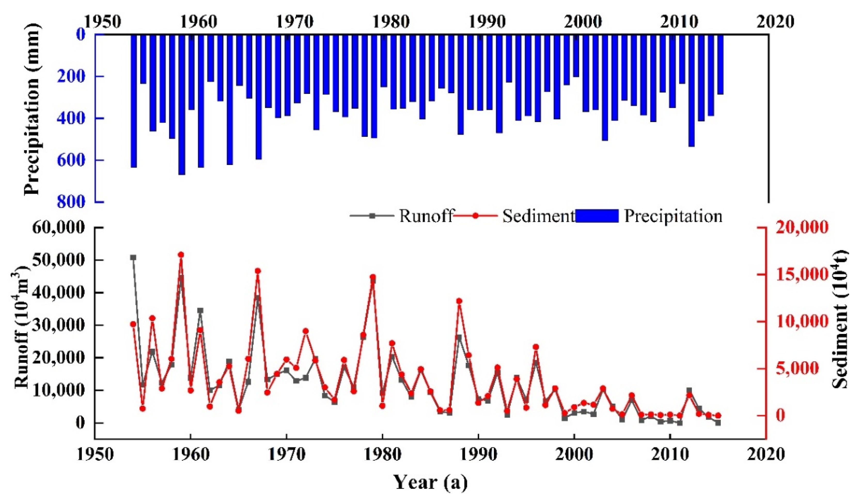
Runoff and sediment discharge are important hydrological information to ensure the ecological security of rivers. To understand the changes between runoff and sediment in the Huangfuchuan watershed over 62 years, the interannual variation of annual precipitation, corresponding annual runoff, and annual sediment in the Huangfuchuan watershed from 1954 to 2015 is plotted, as shown in Figure 2. It can be seen from the figure that the interannual trends of runoff and sediment are basically consistent.
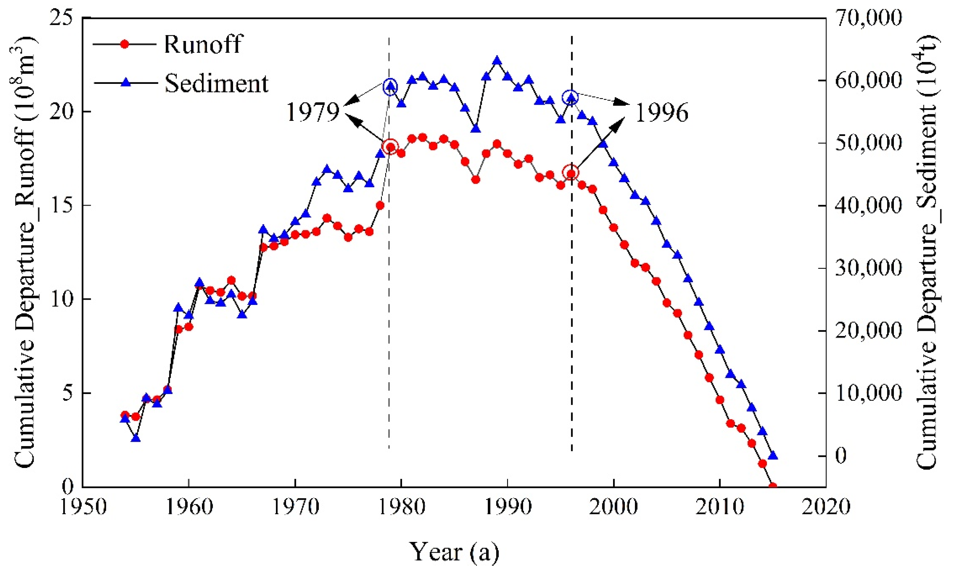
The cumulative anomaly method is used to test the mutation points of the runoff series and sediment series of the Huangfuchuan River basin from 1954 to 2015, and the cumulative anomaly curves of annual runoff and annual sediment discharge in the Huangfuchuan River basin are shown in Figure 3. Observing the trend of cumulative anomaly curves, it can be found that from 1954 to 1978, the cumulative anomaly curves of annual runoff and annual sediment discharge show both fluctuating upward trends, indicating that the runoff and sediment in the Huangfuchuan River basin were in a relatively abundant state during this period. From 1979 to 1996, the cumulative anomaly curves of annual runoff and annual sediment discharge fluctuated but are relatively flat overall, indicating that the Huangfuchuan River basin was in a relatively medium state during this period. From 1997 to 2015, the cumulative anomaly curves of annual runoff and annual sediment discharge show a significant decreasing trend, indicating that the runoff and sediment in the Huangfuchuan River basin were in a relatively low period.
To further determine the year of the mutation, the double mass curve method is adopted to conduct the test of abrupt changes on both the annual runoff series and annual sediment series of the Huangfuchuan River basin, as shown in Figure 4. It can be found that the runoff-sediment accumulation curve of the Huangfuchuan River basin significantly shifted between 1979 and 1996. The period before the shift is generally regarded as the period of no or less disturbance by human activities, i.e., the base period. After the base period, the slope of the accumulation curve changes again, and the slope of the curve decreases, indicating that there is a downward trend of sediment discharge relative to the runoff, so the periods of 1979–1996 and 1997–2015 can be classified as human activity periods. The determination coefficient R2 of the fitted relational equation for each period is above 0.97, which is a good fit.
According to the above two mutation tests, the results of variability analysis can be obtained. The years 1979 and 1996 are the mutation points of the runoff and sediment series in the Huangfuchuan River basin, and the runoff and sediment series in the Huangfuchuan River basin are divided into three stages: 1954–1978 ( T a ), 1979–1996 ( T b ), and 1997–2015 ( T c ). Table 3 shows the results of trend tests for runoff and sediment in the Huangfuchuan River basin at these three stages. It can be seen from the table that there are differences in the trends of annual runoff and sediment discharge at the three stages of division. The  Z s _ M K  value of the M-K trend test for runoff at the stage  T c  is −2.0991,  Z s _ M K  > 1.96, has passed the significance test with a confidence level of 95%. The  Z s _ M K  value of the M-K test for sediment at the stage  T c  is −2.7289,  Z s _ M K  > 2.58, has passed the significance test of 99% confidence level. The statistics of the TFPW_MK test are slightly smaller than those of the M-K test, but the significance and trend are basically consistent. This indicates that the runoff and sediment in the Huangfuchuan River basin show a significant decreasing trend in the  T c  stage (1997–2015). In other periods, the runoff and sediment show a decreasing trend, but the trends are not significant.
The main statistical characteristic values of runoff and sediment discharge in these three stages are given in Table 4. As can be seen from Table 4, the average runoffs are 185.437, 134.775, and 37.676 million cubic meters, respectively, and the average sediments are 58.006, 43.726, and 8.667 million tons, respectively, at the three stages. The runoff and sediment in each stage show a decreasing trend as a whole with the continuation of time, which is consistent with the conclusion obtained by the cumulative anomaly method (Figure 3). The coefficient of variation  C v  represents the degree of dispersion of the data. From the overall perspective, the dispersion degree of sediment discharge is greater than that of runoff, and the dispersion degree of both runoff and sediment discharge tends to increase with the continuation of time at each stage. The skewness coefficient SK describes the degree of distribution deviation from symmetry, and the skewness of both runoff and sediment shows a trend of first increasing and then decreasing in all three stages.
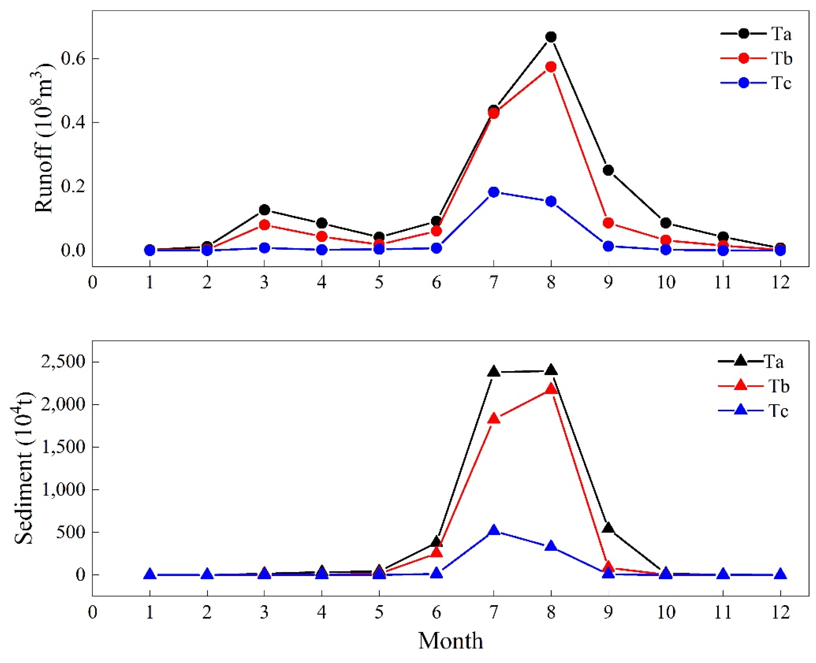
The intra-annual distributions of the mean values of runoff and sediment in three stages of the Huangfuchuan River basin are shown in Figure 5. The runoff and sediment are very unevenly distributed within the year, mainly concentrated in the flood season (June to September), and the sediment discharge in each stage of the flood season accounts for 98.11%, 99.19%, and 99.80% of the annual sediment discharge, respectively, and the runoff in each stage of the flood season accounts for 78.18%, 85.47%, and 95.20% of the annual runoff, respectively. The unevenness of the sediment discharge is greater than that of the runoff.
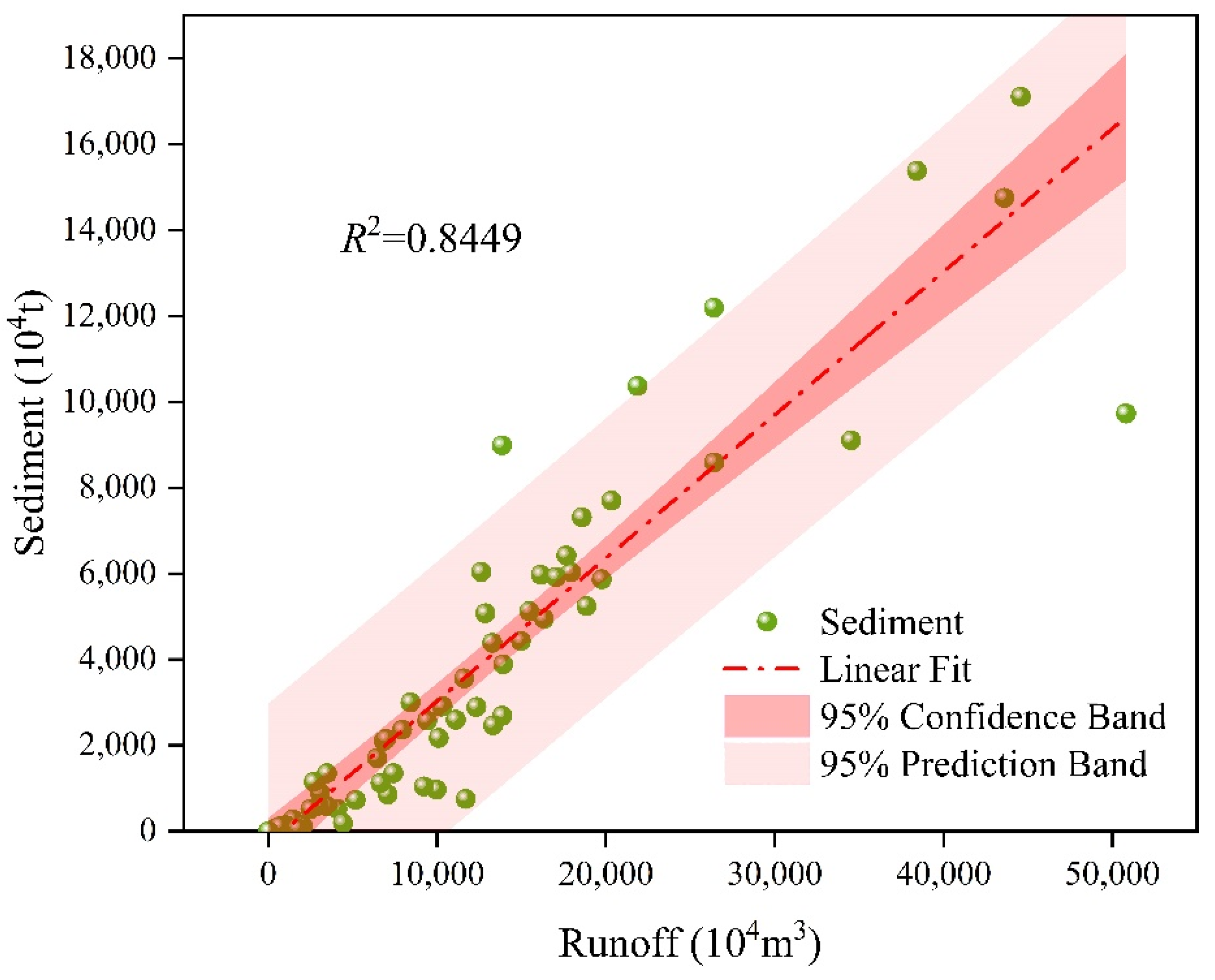
Copula is a joint probability distribution function constructed by connecting the marginal distribution function of related variables. Therefore, the correlation measurement between variables is an important prerequisite. An important step is to draw a correlation analysis chart between runoff and sediment, as shown in Figure 6. The linear fitting correlation coefficient R2 = 0.8449 between runoff and sediment. The vast majority of the correlation analysis point distances between runoff and sediment transport in the Huangfuchuan River Basin are densely distributed near the linear fitting line. The 95% prediction band (estimated to be the area where 95% of the data points belong) relatively evenly includes the linear fitting line, and the point distances of each era are distributed on both sides of the linear fitting line. This indicates that there is no significant systematic deviation in the relationship between water and sediment, and there is a strong correlation between runoff and sediment transport at the Huangfuchuan River basin from 1954 to 2015.
Further, the Pearson linear correlation coefficient γ, the Kendall rank correlation coefficient τ, and the Spearman rank correlation coefficient ρ are adopted to analyze the correlation between the two indicators of runoff and sediment discharge, and the closer the absolute value of the correlation coefficient is to 1, the stronger the correlation between the two variables. According to the calculation results in Table 5, there is a very strong correlation between the runoff and sediment discharge in the three stages. Among them, the Pearson linear correlation coefficients exceed 0.84, the Kendall rank correlation coefficients are over 0.67, and the Spearman rank correlation coefficients surpass 0.85 in the three stages. The basic requirements of the copula function for variables are met.

3.2. Marginal Distributions and Copula Joint Distributions

3.2.1. Selection of Marginal Distributions

Six commonly used theoretical distribution functions, namely, the normal (NOR) distribution function, the gamma (GAM) distribution function, the exponential (EXP) distribution function, the Weibull (WBL) distribution function, the generalized extreme value (GEV) distribution function, the and lognormal (LOGN) distribution function, are used to fit the annual runoff and annual sediment data of the Huangfuchuan River basin, as shown in Table 6.
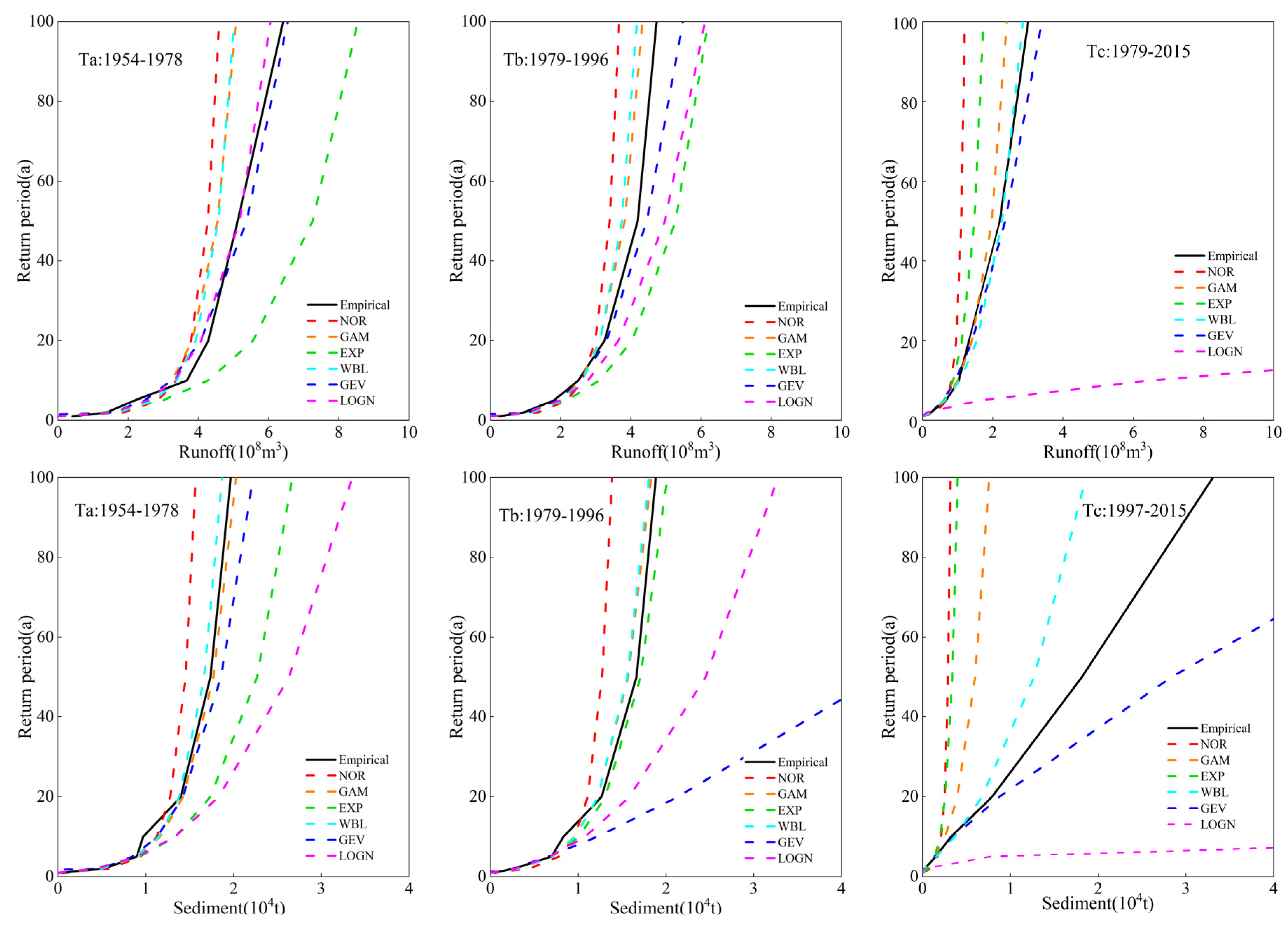
The parameter estimates corresponding to these six marginal distribution functions in the three stages are listed in Table 6, and the K-S test is used to fit the marginal functions. A K-S test result of 0 indicates that the distribution is satisfied by the K-S test. Except for the exponential distribution of runoff in stage    T a  and the lognormal distribution of sediment in stage  T c , the six theoretical distributions can be used to describe the annual runoff and annual sediment discharge in all other stages. The results of OLS and AIC criteria tests are also listed in the table. The test criteria are: The smaller the OLS and AIC values are, the better the fit is. It can be seen from the table that the runoff in stage    T a  obeys the generalized extreme value distribution and the sediment obeys the gamma distribution; the runoff in stage    T b  obeys the generalized extreme value distribution and the sediment obeys the exponential distribution; the runoff in stage    T c  obeys the generalized extreme value distribution and the sediment obeys the generalized extreme value distribution. The comparison of the cumulative probability distribution of the six theoretical distribution functions and the cumulative probability distribution of the empirical distribution functions for runoff and sediment in the three stages are shown in Figure 7. The closer the six theoretical distributions are to the empirical distribution, the better the fitting effect is.

3.2.2. Choice of Copula Joint Distribution

The three copula functions are used to construct the joint distributions of runoff and sediment, using the principles of the OLS, AIC, and BIC, that is, the smaller the value of OLS, AIC, and BIC, the better the fit is. It can be seen from Table 7 that the optimal joint distribution copula functions of runoff and sediment in the  T a  and    T b  stages are both Gumbel, and the optimal joint distribution copula function of runoff and sediment in the stage  T c  is Clayton.
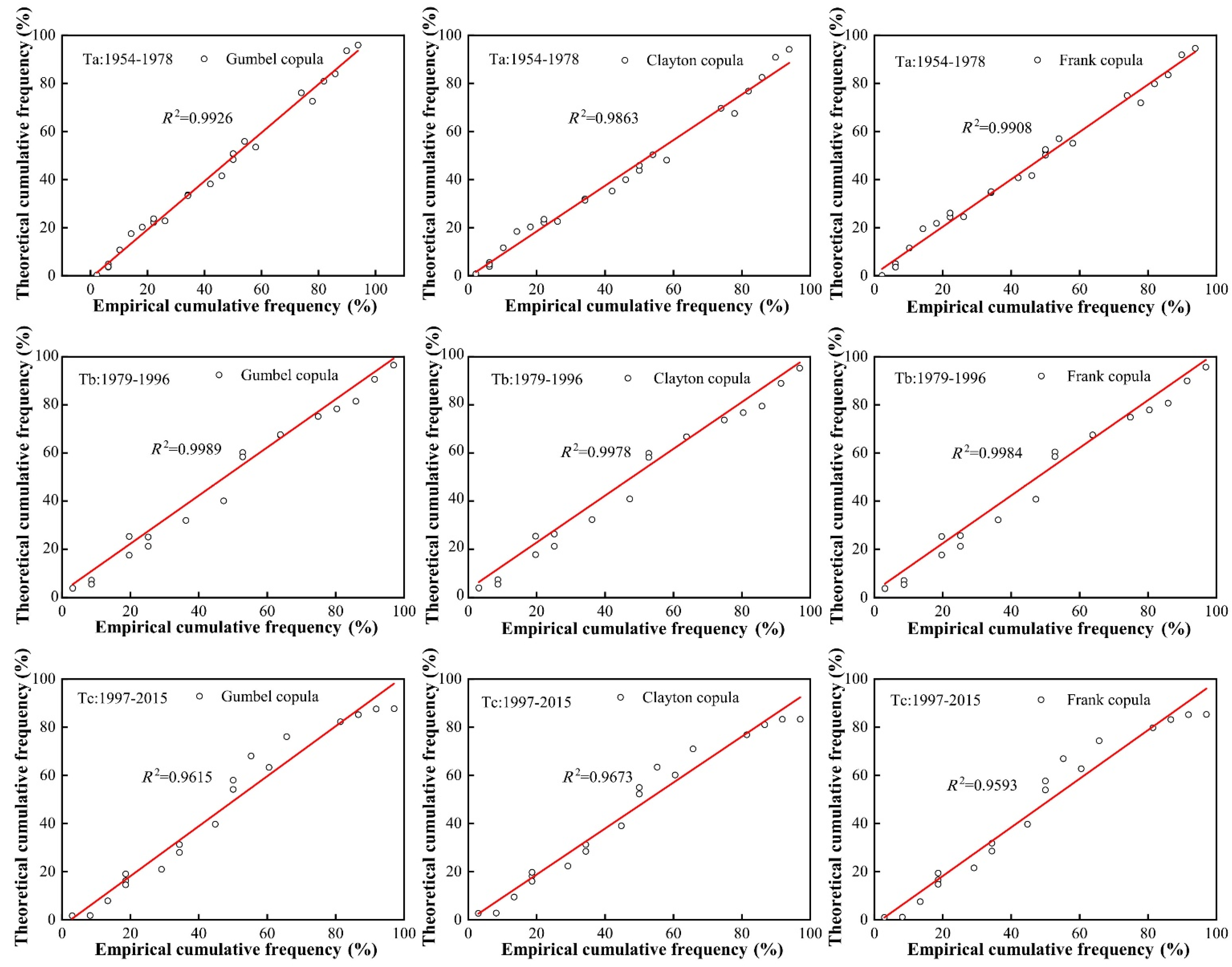
The following figure shows that the empirical cumulative frequencies of three Archimedean copula functions in the three stages are compared with the theoretical cumulative frequency consistency. By calculating R2 and according to the principle of maximum R2 the copula function can be determined as the optimal function. It can be seen from the Figure 8 that all the three copula functions of the three phases fall near the 45° line, and the correlation coefficients are relatively high (all are greater than 0.9593). The Gumbel copula’s fit is the highest for the stage  T a    and the stage  T b . The Clayton copula’s fit is the highest for the stage  T c . These are consistent with the conclusions of OLS, AIC, and BIC tests. That is, Gumbel copula is selected as the optimal copula function to connect the optimal marginal distribution functions of runoff and sediment in the Huangfuchuan River basin in the stages  T a    and  T b , and the Clayton copula is selected as the optimal copula function to connect the optimal marginal distribution functions of runoff and sediment in the Huangfuchuan River basin in the stage  T c .

3.3. Runoff-Sediment Encounter Probability Analysis

The copula joint distribution models of runoff and sediment determined above are applied to study the rich-poor encounter combinations of runoff and sediment at each stage in the Huangfuchuan River basin. The frequency method with  p f  = 37.5% and  p k  = 62.5% as the division frequency is used to classify the runoff and sediment at each stage into three states of rich, normal, and poor, and nine different encounter combinations, respectively, to analyze the changing characteristics of runoff–sediment combination and the encounter probabilities.
It can be seen from Table 8 that: ① The synchronous probabilities of runoff and sediment in different periods are greater than the asynchronous probabilities, which indicates that the runoff and sediment in each stage before and after the mutation points are closely related, with a strong correlation. Among the synchronous probabilities in the three stages, the encounter probabilities of annual rich runoff and rich sediment are the largest, the probabilities of poor runoff and poor sediment are slightly smaller than the probabilities of same rich, and the probabilities of annual normal runoff and normal sediment are the least, which indicates that the synchronization with the same rich is the strongest in the runoff-sediment relationship. ② Due to the symmetry of the copula function, in the asynchronous probabilities, the encounter probabilities of rich runoff and normal sediment are equal to those of normal runoff and rich sediment, rich runoff and poor sediment are equal to those of poor runoff and rich sediment, normal runoff and poor sediment are equal to those of poor runoff and normal sediment. Among them, the encounter probabilities of the combinations of runoff–rich and sediment–poor, as well as runoff–poor and sediment–rich, are the smallest among the six asynchronous probabilities, which indicates that the correlation between the runoff and sediment series is strong, and the probability of occurrence of the two diametrically opposite situations is the smallest. ③ The asynchronous probabilities in the two human activity periods ( T b    and  T c ) are 84.82% and 70.72%, respectively, which are increased compared with the base period ( T a ). This is because the marginal distribution of runoff and sediment variables, the impact mechanism of runoff and sediment, and the relationship between runoff and sediment may have changed to a certain extent under the combined influence of climate change and human activities during the human activity periods. The calculation of the runoff–sediment encounter probability in the Huangfuchuan River basin can further quantify the frequency of runoff and sediment disasters in the Huangfuchuan River basin, which in turn can provide decision-making and guidance for the scientific management of runoff-sediment projects in the Huangfuchuan River basin.

3.4. Return Period Analysis

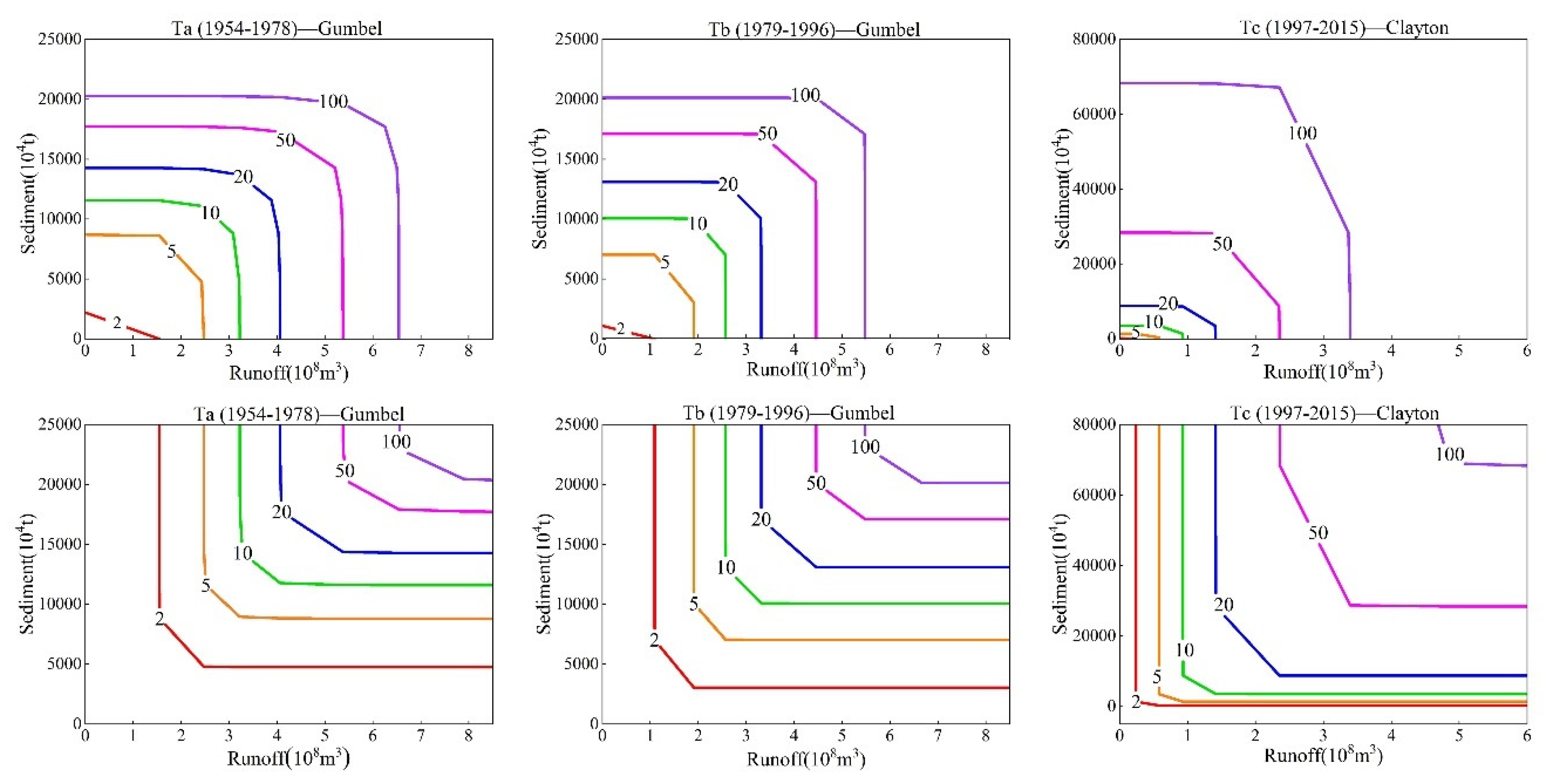
By constructing the two-dimensional copula function of runoff and sediment, the joint return period and the co-occurrence return period of the two-dimensional joint distribution of runoff and sediment are calculated using Equations (8) and (9), and the corresponding return period contours are drawn in Figure 9. It can be seen from the figure that the constructed model can obtain the return periods of different magnitudes of annual runoff and annual sediment discharge encounters combinations in the Huangfuchuan River basin. On this basis, the typical years of runoff and sediment can be selected, and the same frequency amplification method can be used to obtain the runoff and sediment ratio system with different designed runoff hydrographs and designed sediment discharge hydrographs with the same return period, which can provide references for different runoff–sediment conditions selection and generalization in the numerical simulation of the river, hydraulic model testing, and planning and dispatching of downstream cascade hubs.

4. Uncertainty Analysis

In multivariate hydrological analysis, the uncertainty of the results is mainly due to the following reasons: (1) The representativeness of the sample. The difficulty of obtaining the measured sample data and the insufficiency of the sample data length make the sample prone to some deviation in representing the population. (2) The selection of the model function. The differences in the selection of the model function and the determination of the function parameters can cause great uncertainty in the results.

4.1. Uncertainty Analysis of Margin Distributions

The multivariate joint distribution is usually constructed by specifying the univariate marginal distribution and copula function. Determination of the discrete or continuous marginal distribution is the first step of the standard two-step procedure, after which the copula parameters and functions are determined based on the marginal distribution determination [43]. Therefore, it is of great significance to determine a reasonable marginal distribution for the determination of the final joint distribution. The runoff and sediment discharge at each stage of the Huangfuchuan River basin are fitted with six marginal distribution functions. When the return period of runoff and sediment discharge is 0~100 years, the inverse functions of these six marginal distribution functions can be obtained, and the eigenvalues of runoff and sediment discharge corresponding to various return periods can be obtained and compared with those of the empirical distribution (Figure 9). It can be seen from Figure 10 that there are significant differences between different marginal distribution functions. In stage    T a , the return periods of runoff obtained from the generalized extreme value distribution and the lognormal distribution are the closest to those obtained from the empirical distribution, and both pass the K-S test, with the smallest values of the OLS and AIC criteria for the generalized extreme value distribution; the return periods of sediment discharge obtained from the generalized extreme value distribution, the Weibull distribution, and the gamma distribution are the closest to those obtained from the empirical distribution, and they all pass the K-S test, with the smallest values of the OLS and AIC criteria for the gamma distribution. In stage    T b , the return period of runoff obtained from the generalized extreme value distribution is the closest to that obtained from the empirical distribution, and the return period of sediment discharge obtained from the exponential distribution is the closest to that obtained from the empirical distribution, and both distributions pass the K-S test; their OLS and AIC criterion values are also the smallest. In stage    T c , the return periods obtained from the generalized extreme value distribution for both runoff and sediment are the closest to those obtained from the empirical distribution, and both distributions pass the K-S test; their OLS and AIC criterion values are also the smallest. These validation results indicate that runoff and sediment discharge fitting different marginal distribution functions differ significantly and that the univariate characteristic return periods are sensitive to the selection of marginal distribution functions.

4.2. Uncertainty Analysis of Parameters

In multivariate hydrological analysis, the selection of function parameters determines the correctness of the function and the accuracy of the results. The Monte Carlo method is a commonly used method for analyzing uncertainty problems based on probability statistics. To address the uncertainty of the selected model parameters, the Monte Carlo method [44,45] is chosen in this paper to resample the samples several times to assess the impact of parameter uncertainty on the model. The specific method is based on the joint distribution model of the copula function generated at each stage, selecting binary samples with the same length as the observation values, and applying the Monte Carlo method to simulate, with the simulation times set to 1000. The maximum likelihood estimation method is used to estimate the parameters of the marginal distribution and the runoff–sediment joint distribution model based on the simulated samples. The box plot of the simulated parameter values is shown in Figure 11. In the stage  T a , the runoff marginal function is the generalized extreme value (GEV) function, whose parameters are shape parameter κ, scale parameter α, and location parameter ξ; the sediment marginal function is the gamma (GAM) function, whose parameters are shape parameter  α 1 , scale parameter  α 2 ; and the copula function is the Gumbel function with parameter θ. In the stage  T b , the runoff marginal function is the generalized extreme value (GEV) function, whose parameters are shape parameter κ, scale parameter α, and location parameter ξ; the sediment marginal function is the exponential (EXP) function, with parameter μ, and the copula function is the Gumbel function with parameter θ. In the stage    T c , the marginal functions of both runoff and sediment are the generalized extreme value (GEV) functions with parameters κ, α, and ξ, and the copula function is a Clayton function with parameter θ. It can be seen from Figure 10 that the parameters of the marginal distributions and joint distributions based on the observation values locate in the range of the simulation parameters, which are close to the mean position. Therefore, it can be concluded that the parameters selected in determining the marginal distributions and copula functions are reasonable.

4.3. Uncertainty Analysis of Copula Functions

Every copula has its own specific dependence structure [46]. The difference in the selection of the copula function has a great impact on the calculation results. Selecting a reasonable copula function is the key to constructing the joint distribution function [47]. The aforementioned copula functions are used to construct the joint distribution functions of runoff and sediment, and the differences between the three copula functions are analyzed. Since both runoff and sediment obey six marginal distributions, each year corresponds to 108 joint distribution functions, and the co-occurrence return period and joint return period of runoff and sediment corresponding to the 108 joint distributions can be calculated. For example, the year 1961 is selected for analysis, which is in the stage    T a . The annual runoff is 345.160 million m3 and the annual sediment discharge is 91.037 million tons in that year. Three copula functions are used to construct the joint distribution function of runoff and sediment, and the runoff and sediment discharge are also subject to the six marginal distributions mentioned above. When the Gumbel copula function is obeyed, the range of the co-occurrence return period is 5.06~13.64 years; when the Clayton copula function is obeyed, the range of the co-occurrence return period is 6.38–30.88 years; when the Frank copula function is obeyed, the range of the co-occurrence return period is 5.66–19.14 years. From the variation range of the co-occurrence return period, it can be seen that the corresponding results of the three Copula functions are quite different. The optimal marginal distribution functions of runoff and sediment are generalized extreme value (GEV) distribution and gamma (GAM) distribution, and the optimal copula function is the Gumbel copula in the stage    T a . The co-occurrence return period of runoff and sediment corresponding to the optimal marginal distribution and the optimal copula function is 10.89 years, while the empirical co-occurrence period of runoff and sediment in 1961 is 10.16 years, which are close to each other, indicating that the selection of the copula function is correct. Therefore, it is significant to select the appropriate copula function for constructing the optimal joint distribution function.

5. Discussions

Many studies have shown that climate change and human activities are important factors that cause changes in runoff and sediment, as well as changes in the runoff–sediment relationship. Therefore, it is necessary to study the response of runoff and sediment to climate and human activities. Many meteorological factors are closely related to changes in runoff and sediment. Precipitation and temperature are selected as representatives of meteorological factors, which act on hydrological cycles and directly or indirectly affect the process of runoff and sediment. It is important to calculate the Pearson correlation coefficient between runoff (sediment) and selected meteorological factors and analyze the impact of climate change (precipitation and temperature) on runoff and sediment changes and runoff-sediment relationships in the Huangfuchuan River basin. The calculation results are shown in Table 9.
As shown in Table 9, there are significant differences in the impact factors on runoff and sediment at each stage, but there are still certain regularities. Among them, precipitation in each stage has a strong correlation with runoff and sediment, but the correlation gradually weakens over time, and the correlation between runoff (sediment) and temperature in each stage is relatively small. In other words, the dynamic change of runoff and sediment is mainly driven by precipitation, and temperature is also one of the indispensable reasons for the change of runoff and sediment. In recent decades, the climate in the Huangfuchuan River basin has shown a relatively obvious trend of warming and drying, which is one of the important reasons for the reduction of runoff and sediment in the Huangfuchuan River basin.
Human activities usually have an impact on the underlying surface of a watershed through methods such as soil and water conservation, urban construction, and domestic production water use. The changes in underlying surface conditions are mainly reflected in land use methods, vegetation cover changes, and water conservancy engineering measures. The construction of check dams is one of the important measures for soil erosion control in the Huangfuchuan River basin. The check dam project can effectively regulate runoff and play a role in reducing flood and sediment. Since the 1950s, soil and water conservation management has been carried out in the Huangfuchuan River basin, with the construction of check dams. However, due to the use of traditional farming methods and the small proportion of remaining storage capacity of check dams before 2000, most of them have already been silted and become ineffective. Therefore, the control speed is relatively slow, and the effect is not significant. Compared with the base period, the synchronous frequency of runoff and sediment increased, while the asynchronous frequency decreased in the stage    T b . The frequency of rich runoff and rich sediment, normal runoff and normal sediment, poor runoff and poor sediment all increased, indicating that although soil and water conservation measures at this stage have played a role in reducing runoff and sediment to a certain extent (Table 4), they have not made a contribution to regulating the coupling relationship between water and sediment.
Vegetation can intercept precipitation, increase infiltration, and play a role in reducing flood peaks and erosion. In 1999, the Huangfuchuan River basin started a large-scale project of returning cropland to forests and grassland. The normalized vegetation index (NDVI) showed an upward trend, with an increase rate of 0.095/10a. After 2000, the construction of check dams was further strengthened. By 2015, the number of check dams in the Huangfuchuan River basin had increased to 886, with a total storage capacity of 493 million m3, and the proportion of dam-controlled area in the basin reached 70%. Therefore, compared with the stage  T b , the synchronous frequency of runoff-sediment (especially the frequency of the same rich and same normal) in stage  T c  significantly decreased, while the asynchronous frequency of runoff–sediment increased during the same period, indicating that soil and water conservation measures in this stage not only reduced runoff and sediment, but also effectively reduced the sediment content of rich runoff, reduced co-occurrence probability, and adjusted the probability of extreme runoff and sediment events.
6. Conclusions

In this paper, the Huangfuchuan River basin in the middle reaches of the Yellow River is taken as the research object, and a joint distribution model of runoff and sediment is constructed by using the copula theory. The characteristics of rich–poor encounter combinations of runoff and sediment are analyzed, the encounter probabilities under each scenario are identified, and the uncertainty factors in the process of constructing the Copula joint distribution function are discussed. The main conclusions are given as follows:
(1)
Based on the cumulative anomaly method and the double mass curve method, 1979 and 1996 are identified as mutation points of runoff and sediment series in the Huangfuchuan River basin, and the runoff and sediment series in the Huangfuchuan River basin are divided into three stages. The runoff and sediment in all three stages show a strong correlation.
(2)
Based on the results of K-S, OLS, and AIC criteria tests, the runoff in the Huangfuchuan River basin obeys the GEV distribution and the sediment obeys the GAM distribution in the stage  T a ; the runoff obeys the GEV distribution and the sediment obeys the EXP distribution in the stage  T b ; the runoff and sediment obey the GEV distribution in the stage  T c . Based on the results of OLS, AIC, and BIC criteria tests, the Gumbel copula is selected as the optimal joint distribution function of runoff and sediment in the stages  T a  and  T b , and the Clayton copula is selected as the optimal joint distribution function of runoff and sediment in the stage  T c .
(3)
The synchronous probabilities in the three stages are 69.84%, 84.82%, and 70.72%, respectively, which are much greater than the asynchronous probabilities, indicating a strong consistency of runoff and sediment in the River basin. The synchronous probabilities in the stages  T b  and  T c  have increased compared with those in stage  T a , indicating that under the combined influence of climate change and human activities, the impact mechanism of runoff–sediment has become more complex and the relationship between runoff and sediment may have changed to a certain extent.
(4)
The contour maps of the joint return period and the co-occurrence return period of the two-dimensional joint distribution of runoff and sediment discharge are drawn. On this basis, the typical years of runoff and sediment can be selected, and the same frequency amplification method can be used to obtain the runoff and sediment ratio system with different designed runoff hydrographs and designed sediment discharge hydrographs with the same return period.
(5)
The uncertainties and sensitivities of the joint distribution function construction process are analyzed, showing that the optimal marginal distribution functions, the optimal copula functions, and the parameters selected by the great likelihood estimation method can better fit the runoff–sediment relationship in the river basin and reduce the process uncertainties.

Author Contributions

X.H.: conceptualization, writing-draft preparation, methodology; L.Q.: review and editing, supervision. All authors have read and agreed to the published version of the manuscript.

Funding

The research was funded by the Project of key science and technology of the Henan province (No: 222102320333), Henan province university scientific and technological innovation team (No: 18IRTSTHN009).

Data Availability Statement

Not applicable.

Acknowledgments

Thank all the authors for their contributions.

Conflicts of Interest

The authors declare no conflict of interest.

References

  1. Li, L.; Wu, K.; Jiang, E.; Yin, H.; Wang, Y.; Tian, S.; Dang, S. Evaluating Runoff-Sediment Relationship Variations Using Generalized Additive Models That Incorporate Reservoir Indices for Check Dams. Water Resour. Manag. 2021, 35, 3845–3860. [Google Scholar] [CrossRef]
  2. Zhang, X.; Lin, P.; Chen, H.; Yan, R.; Zhang, J.; Yu, Y.; Liu, E.; Yang, Y.; Zhao, W.; Lv, D.; et al. Understanding land use and cover change impacts on run-off and sediment load at flood events on the Loess Plateau, China. Hydrol. Process. 2018, 32, 576–589. [Google Scholar] [CrossRef]
  3. Phillips, M.C.; Solo-Gabriele, H.M.; Piggot, A.M.; Klaus, J.S.; Zhang, Y. Relationships between sand and water quality at recreational beaches. Water Res. 2011, 45, 6763–6769. [Google Scholar] [CrossRef] [PubMed] [Green Version]
  4. Guo, A.; Chang, J.; Wang, Y.; Huang, Q.; Zhou, S. Flood risk analysis for flood control and sediment transportation in sandy regions: A case study in the Loess Plateau, China. J. Hydrol. 2018, 560, 39–55. [Google Scholar] [CrossRef]
  5. Tian, P.; Zhai, J.; Zhao, G.; Mu, X. Dynamics of Runoff and Suspended Sediment Transport in a Highly Erodible Catchment on the Chinese Loess Plateau. Land Degrad. Dev. 2015, 27, 839–850. [Google Scholar] [CrossRef]
  6. Li, R.; Zhu, A.; Song, X.; Cui, M. Seasonal Dynamics of Runoff-Sediment Relationship and Its Controlling Factors in Black Soil Region of Northeast China. J. Resour. Ecol. 2010, 1, 345–352. [Google Scholar]
  7. Thanh Son Ngo, D.B.N.P.S.R. Effect of land use change on runoff and sediment yield in Da River Basin of Hoa Binh province, Northwest Vietnam. J. Mt. Sci. 2015, 12, 1051–1064. [Google Scholar]
  8. Guo, A.; Chang, J.; Wang, Y.; Huang, Q. Variations in the Runoff-Sediment Relationship of the Weihe River Basin Based on the Copula Function. Water 2016, 8, 223. [Google Scholar] [CrossRef] [Green Version]
  9. Wen, Y.; Yang, A.; Kong, X.; Su, Y. A Bayesian-Model-Averaging Copula Method for Bivariate Hydrologic Correlation Analysis. Front. Environ. Sci. 2022, 9, 744462. [Google Scholar] [CrossRef]
  10. Trinh, T.; Ishida, K.; Kavvas, M.L.; Ercan, A.; Carr, K. Assessment of 21st century drought conditions at Shasta Dam based on dynamically projected water supply conditions by a regional climate model coupled with a physically-based hydrology model. Sci. Total Environ. 2017, 586, 197–205. [Google Scholar] [CrossRef]
  11. Ho, C.; Trinh, T.; Nguyen, A.; Nguyen, Q.; Ercan, A.; Kavvas, M.L. Reconstruction and evaluation of changes in hydrologic conditions over a transboundary region by a regional climate model coupled with a physically-based hydrology model: Application to Thao river watershed. Sci. Total Environ. 2019, 668, 768–779. [Google Scholar] [CrossRef] [PubMed]
  12. Todorovic, P. Stochastic Models of Floods. Water Resour. Res. 1978, 14, 345–356. [Google Scholar] [CrossRef]
  13. Remesan, R.; Shamim, M.A.; Han, D.; Mathew, J. Runoff prediction using an integrated hybrid modelling scheme. J. Hydrol. 2009, 372, 48–60. [Google Scholar] [CrossRef]
  14. Fan, Y.; Huang, G.; Zhang, Y.; Li, Y. Uncertainty Quantification for Multivariate Eco-Hydrological Risk in the Xiangxi River within the Three Gorges Reservoir Area in China. Engineering 2018, 4, 617–626. [Google Scholar] [CrossRef]
  15. Goel, N.K.; Seth, S.M.; Chandra, S. Multivariate Modeling of flood flows. J. Hydraul. Eng. 1998, 124, 146–155. [Google Scholar] [CrossRef]
  16. Yue, S.; Rasmussen, P. Bivariate frequency analysis: Discussion of some useful concepts in hydrological application. Hydrol. Process. 2002, 16, 2881–2898. [Google Scholar] [CrossRef]
  17. Vinnarasi, R.; Dhanya, C.T. Bringing realism into a dynamic copula-based non-stationary intensity-duration model. Adv. Water Resour. 2019, 130, 325–338. [Google Scholar] [CrossRef]
  18. Zhang, L.; Chen, Y.; Wang, Y.; Bai, Y. Probabilistic analysis of the controls on groundwater depth using Copula Functions. Hydrol. Res. 2020, 51, 406–422. [Google Scholar]
  19. Abdollahi, S.; Akhoond-Ali, A.M.; Mirabbasi, R.; Adamowski, J.F. Probabilistic Event Based Rainfall-Runoff Modeling Using Copula Functions. Water Resour. Manag. 2019, 33, 3799–3814. [Google Scholar] [CrossRef]
  20. Grimaldi, S.; Petroselli, A.; Salvadori, G.; De Michele, C. Catchment compatibility via copulas: A non-parametric study of the dependence structures of hydrological responses. Adv. Water Resour. 2016, 90, 116–133. [Google Scholar] [CrossRef]
  21. Xiong, L.; Yu, K.-X.; Gottschalk, L. Estimation of the distribution of annual runoff from climatic variables using copulas. Water Resour. Res. 2014, 50, 7134–7152. [Google Scholar] [CrossRef]
  22. Perz, A.; Sobkowiak, L.; Wrzesiński, D. Probabilistic Approach to Precipitation-Runoff Relation in a Mountain Catchment: A Case Study of the Kłodzka Valley in Poland. Water 2021, 13, 1229. [Google Scholar] [CrossRef]
  23. Sugimoto, T.; Bárdossy, A.; Pegram, G.G.S.; Cullmann, J. Investigation of hydrological time series using copulas for detecting catchment characteristics and anthropogenic impacts. Hydrol. Earth Syst. Sci. 2016, 20, 2705–2720. [Google Scholar] [CrossRef] [Green Version]
  24. Golian, S.; Saghafian, B.; Farokhnia, A.; Rivard, C. Copula-based interpretation of continuous rainfall–runoff simulations of a watershed in northern Iran. Can. J. Earth Sci. 2012, 49, 681–691. [Google Scholar] [CrossRef]
  25. Bacchi, B.; Balistrocchi, M. Derivation of flood frequency curves through a bivariate rainfall distribution based on copula functions: Application to an urban catchment in northern Italy’s climate. Hydrol. Res. 2017, 48, 749–762. [Google Scholar]
  26. Requena, A.I.; Flores, I.; Mediero, L.; Garrote, L. Extension of observed flood series by combining a distributed hydro-meteorological model and a copula-based model. Stoch. Environ. Res. Risk Assess. 2015, 30, 1363–1378. [Google Scholar] [CrossRef] [Green Version]
  27. Chang, J.; Li, Y.; Wang, Y.; Yuan, M. Copula-based drought risk assessment combined with an integrated index in the Wei River Basin, China. J. Hydrol. 2016, 540, 824–834. [Google Scholar] [CrossRef]
  28. Li, Y.; Cai, Y.; Li, Z.; Wang, X.; Fu, Q.; Liu, D.; Sun, L.; Xu, R. An approach for runoff and sediment nexus analysis under multi-flow conditions in a hyper-concentrated sediment river, Southwest China. J. Contam. Hydrol. 2020, 235, 103702. [Google Scholar] [CrossRef]
  29. Dodangeh, E.; Shahedi, K.; Pham, B.T.; Solaimani, K. Joint frequency analysis and uncertainty estimation of coupled rainfall–runoff series relying on historical and simulated data. Hydrol. Sci. J. 2019, 65, 455–469. [Google Scholar] [CrossRef]
  30. Salvadori, G.; Durante, F.; De Michele, C.; Bernardi, M.; Petrella, L. A multivariate copula-based framework for dealing with hazard scenarios and failure probabilities. Water Resour. Res. 2016, 52, 3701–3721. [Google Scholar] [CrossRef] [Green Version]
  31. Razmkhah, H.; AkhoundAli, A.-M.; Radmanesh, F. Correlated Parameters Uncertainty Propagation in a Rainfall-Runoff Model, Considering 2-Copula; Case Study: Karoon III River Basin. Environ. Model. Assess. 2017, 22, 503–521. [Google Scholar] [CrossRef]
  32. Zimmermann, H.J. Fuzzy Set Theory—And Its Applications; Kluwer Academic Pub: Dordrecht, The Netherlands, 2001. [Google Scholar]
  33. Serinaldi, F. Can we tell more than we can know? The limits of bivariate drought analyses in the United States. Stoch. Environ. Res. Risk Assess. 2015, 30, 1691–1704. [Google Scholar] [CrossRef]
  34. Wang, J.; Shi, B.; Zhao, E.; Yuan, Q.; Chen, X. The long-term spatial and temporal variations of sediment loads and their causes of the Yellow River Basin. Catena 2022, 209, 105850. [Google Scholar] [CrossRef]
  35. Liu, X.; Zhang, Y.; Liu, Y.; Zhao, X.; Zhang, J.; Rui, Y. Characteristics of temperature evolution from 1960 to 2015 in the Three Rivers’ Headstream Region, Qinghai, China. Sci. Rep. 2020, 10, 20272. [Google Scholar] [CrossRef]
  36. Yi, W.; Feng, Y.; Liang, S.; Kuang, X.; Yan, D.; Wan, L. Increasing annual streamflow and groundwater storage in response to climate warming in the Yangtze River source region. Environ. Res. Lett. 2021, 16, 084011. [Google Scholar] [CrossRef]
  37. Rozbeh, S.; Adamowski, J.; Darabi, H.; Golshan, M.; Pirnia, A. Using the Mann–Kendall test and double mass curve method to explore stream flow changes in response to climate and human activities. J. Water Clim. Chang. 2019, 10, 725–742. [Google Scholar]
  38. Kendall, M.G. Rank Correlation Methods; Charles Griffin: London, UK, 1975. [Google Scholar]
  39. Mann, H.B. Nonparametric Tests Against Trend. Econometrica 1945, 13, 245–259. [Google Scholar] [CrossRef]
  40. Yue, S.; Pilon, P.; Phinney, B.; Cavadias, G. The influence of autocorrelation on the ability to detect trend in hydrological series. Hydrol. Process. 2002, 16, 1807–1829. [Google Scholar] [CrossRef]
  41. Akalke, H. A New Look at the Statistical Model Identification. IEEE Trans. Autom. Control 1974, 19, 716–723. [Google Scholar]
  42. Sklar, A. Fonctions de Repartition a n Dimensions et Leurs Marges; Publications de l’Institut Statistique de l’Université de Paris: Paris, France, 1959. [Google Scholar]
  43. Silva, R.d.S.; Lopes, H.F. Copula, marginal distributions and model selection: A Bayesian note. Stat. Comput. 2008, 18, 313–320. [Google Scholar] [CrossRef]
  44. Quinton, A.V.J. Sensitivity analysis of EUROSEM using Monte Carlo simulation I:hydrological, soil and vegetation parameters. Hydrol. Process. 2000, 14, 915–926. [Google Scholar]
  45. Borges, C.; Palma, C.; Dadamos, T.; Bettencourt da Silva, R.J.N. Evaluation of seawater composition in a vast area from the Monte Carlo simulation of georeferenced information in a Bayesian framework. Chemosphere 2021, 263, 128036. [Google Scholar] [CrossRef] [PubMed]
  46. Tang, X.-S.; Li, D.-Q.; Rong, G.; Phoon, K.-K.; Zhou, C.-B. Impact of copula selection on geotechnical reliability under incomplete probability information. Comput. Geotech. 2013, 49, 264–278. [Google Scholar] [CrossRef]
  47. Nguyen, D.D.; Jayakumar, K.V. Assessing the copula selection for bivariate frequency analysis based on the tail dependence test. J. Earth Syst. Sci. 2018, 127, 92. [Google Scholar] [CrossRef] [Green Version]
Figure 1. Location map of the study area.
Water 15 02644 g001
Figure 2. Interannual variation characteristics of precipitation, runoff, and sediment from 1954 to 2015.
Water 15 02644 g002
Figure 3. Cumulative anomaly curves of runoff and sediment.
Water 15 02644 g003
Figure 4. Runoff-sediment double mass curve.
Water 15 02644 g004
Figure 5. Intra-annual distribution of runoff and sediment discharge in every stage.
Water 15 02644 g005
Figure 6. Correlation analysis of runoff and sediment.
Water 15 02644 g006
Figure 7. Fitting of marginal distribution functions of runoff and sediment in each stage.
Water 15 02644 g007
Figure 8. The probability–probability plot of the joint distributions.
Water 15 02644 g008
Figure 9. Co-occurrence return period and joint return period of the optimal copula.
Water 15 02644 g009
Figure 10. The return periods based on different marginal distributions.
Water 15 02644 g010
Figure 11. Parameters of marginal distributions and copula functions at each stage.
Water 15 02644 g011
Table 1. Common Archimedean copulas.
Copulas   C u , v Parameters
Gumbel   exp ln u θ + ln v θ 1 / θ θ ≥ 0
Clayton   u θ + v θ 1 1 / θ θ ≠ 0
Frank   1 θ ln 1 + e θ u 1 e θ v 1 e θ 1 θ ≥ 1
Table 2. Encounter combination of rich-poor runoff and sediment.
Runoff
RichNormalPoor
SedimentRich   P 1 = p R r p f , S s p f   P 2 = p r p k < R < r p f , S s p f   P 3 = p R r p k , S s p f
Normal   P 4 = p R r p f , s p k < S < s p f   P 5 = p r p k < R < r p f , s p k < S < s p f   P 6 = p R r p k , s p k < S < s p f
Poor   P 7 = p R r p f , S s p k   P 8 = p r p k < R < r p f , S s p k   P 9 = p R r p k , S s p k
Note: R represents runoff; S represents sediment discharge;  r p f  ( s p f ) represents the rich runoff (sediment) determined by the frequency of 37.5%;  r p k  ( s p k ) represents the poor runoff (sediment) determined by the frequency of 62.5%.
Table 3. Statistical characteristics of runoff and sediment at each stage.
Statistic   T a   T b   T c 1954~2015
RunoffSedimentRunoffSedimentRunoffSedimentRunoffSediment
  Z s _ M K −0.9576−0.4437−1.1363−0.8333−2.0991 **−2.7289 ***−5.7825 ***−5.3209 ***
  Z S _ T F P W −0.3721−0.0758−0.5355−0.1236−1.8939 *−2.6514 ***−5.4948 ***−5.1339 ***
Note: *, **, and *** represent significance at 90%, 95%, and 99% confidence levels corresponding to critical z values of 1.65, 1.96, and 2.58, respectively.
Table 4. Statistical characteristics of runoff and sediment in each stage.
StageCharacteristic VariablesMeanMaximumMinimumStandard Deviation   C v   S K
  T a Runoff ( M C M )185.43750841.080115.2470.6211.534
Sediment ( M T )58.006171.0715.22441.6390.7181.153
  T b Runoff ( M C M )134.775435.94025.11096.9650.7191.699
Sediment ( M T )43.726147.5075.15539.6080.9061.337
  T c Runoff ( M C M )37.676103.449034.4750.9150.886
Sediment ( M T )8.66729.07609.7021.1191.058
Table 5. Correlation coefficients between the runoff and sediment.
Correlation Coefficient   T a   T b   T c
γ0.8440.9700.924
τ0.6730.8950.801
ρ0.8500.9730.919
Note: γ denotes the Pearson linear correlation coefficient, τ represents the Kendall rank correlation coefficient, and ρ indicates the Spearman rank correlation coefficient.
Table 6. Parameters estimation and goodness of fit of the marginal distribution.
MarginParameters and TestsStage
  T a   T b   T c
RunoffSedimentRunoffSedimentRunoffSediment
Normalμ1.8545800.6001.3484372.6000.377866.706
σ1.1764249.7000.9984075.6000.354996.833
K-S000000
OLS0.1230.0770.0890.0970.0960.121
AIC−100.778−123.977−82.909−79.885−84.932−76.369
Gamma   α 1 3.1941.8002.1511.2000.5380.300
  α 2 0.5813257.6000.6273609.5000.7002867.300
K-S000000
OLS0.0820.0410.0510.0550.06000.087
AIC−120.950−155.961−103.278−100.280−103.138−88.927
Exponentialμ1.85445800.6001.3484372.6000.377866.706
K-S100000
OLS0.1360.0710.0830.0390.0470.142
AIC−95.876−128.155−85.526−112.704−112.415−70.276
Weibull   α 1 2.0996386.9001.5014549.1000.326514.919
  α 2 1.7531.4001.4941.1000.7030.426
K-S000000
OLS0.0930.0430.0540.0530.0510.085
AIC−114.895−153.718−101.288−101.493−108.963−89.825
Generalized Extreme Value   κ 0.2160.1000.2130.8000.4881.256
α0.6662850.6000.5911712.9000.187265.187
ξ1.2943724.4000.8651787.8000.165167.711
K-S000000
OLS0.0540.0430.0480.0620.0430.067
AIC−142.254−152.881−105.071−95.941−115.704−98.983
Lognormalμ0.4538.3590.0487.917−2.1434.486
σ0.5800.8860.7571.0673.1235.306
K-S000001
OLS0.0620.0520.0490.0530.1390.161
AIC−135.023−143.847−104.694−101.602−71.133−65.324
Note: Bold indicates the selected Marginal distribution function.
Table 7. Parameters estimation and fitting evaluation of the copula function.
CopulaParameters and TestsStage
  T a   T b   T c
Gumbel   θ 1 2.8246.0623.674
OLS0.0260.0390.061
AIC−178.881−112.607−102.371
BIC−176.444−110.826−100.482
Clayton   θ 2 1.9843.5753.638
OLS0.0440.0580.057
AIC−151.894−98.698−105.086
BIC−149.457−96.917−103.197
Frank   θ 3 10.93723.92711.485
OLS0.0270.0400.061
AIC−175.828−112.037−102.050
BIC−173.390−110.256−100.161
Note: Bold indicates the selected copula function.
Table 8. The encounter probabilities of runoff and sediment.
StageSynchronous Probability (%)Asynchronous Probability (%)
Rich–RichNormal–NormalPoor–PoorTotalRich–NormalRich–PoorNormal–RichNormal–PoorPoor–RichPoor–NormalTotal
  T a 29.8411.4628.5469.846.121.546.127.421.547.4230.16
  T b 34.0417.4833.3084.823.390.073.394.130.074.1315.18
  T c 28.0211.5731.1370.728.251.228.255.171.225.1729.28
Table 9. Correlation coefficient between meteorological factors and runoff (sediment).
Item   T a   T b   T c
PrecipitationTemperaturePrecipitationTemperaturePrecipitationTemperature
Runoff0.859 **−0.1370.773 **−0.0080.619 **−0.173
Sediment0.773 **−0.2350.745 **−0.0510.498 *−0.065
Note: * indicates passing the 0.05 significance level test, and ** indicates passing the 0.01 significance level test.
Disclaimer/Publisher’s Note: The statements, opinions and data contained in all publications are solely those of the individual author(s) and contributor(s) and not of MDPI and/or the editor(s). MDPI and/or the editor(s) disclaim responsibility for any injury to people or property resulting from any ideas, methods, instructions or products referred to in the content.