Article

Representation of Hydrological Components under a Changing Climate—A Case Study of the Uruguay River Basin Using the New Version of the Soil and Water Assessment Tool Model (SWAT+)

by
Osvaldo Luis Barresi Armoa
1,*,
Sabine Sauvage
1,
Tobias Houska
2,
Katrin Bieger
3,
Christoph Schürz
4 and
José Miguel Sánchez Pérez
1,*
1
Laboratoire Ecologie Fonctionnelle et Environnement, Institut National Polytechnique de Toulouse (INPT), Centre National de la Recharche Scientifique (CNRS), Université de Toulouse (UPS), 31326 Toulouse, France
2
Department of Landscape Ecology and Resources Management, Justus Liebig University, 35390 Gießen, Germany
3
Department of Ecoscience—Catchment Science and Environmental Management, Aarhus University, 8000 Aarhus, Denmark
4
Department Computational Landscape Ecology, UFZ—Helmholtz-Centre for Environmental Research, 04318 Leipzig, Germany
*
Authors to whom correspondence should be addressed.
Water 2023, 15(14), 2604; https://doi.org/10.3390/w15142604
Submission received: 12 June 2023 / Revised: 4 July 2023 / Accepted: 11 July 2023 / Published: 18 July 2023

Abstract

:
SWAT+ is a revised version of the SWAT model that has the capability to route flow across landscape units in the catchment, which is expected to improve the spatial representation of processes in watersheds. We applied the SWAT+ model in the Uruguay River Basin, an international river basin in South America with a total surface area of 370,000 km2, in order to (1) assess the water balance components, (2) represent their spatial distribution, and (3) examine their changes over time. The catchment was divided into uplands and floodplains and a decision table rule was developed based on streamflow data. The SPOTPY Python library was linked to SWAT+ and used as a tool to perform sensitivity analyses and calibration. The model represented the fluctuations of discharge well, although there was a general tendency to underestimate peak flows. Blue (precipitation and runoff) and green (evapotranspiration and soil water content) hydrological components were spatially plotted. Overall, SWAT+ simulated a realistic spatial distribution of the water cycle components. A seasonal Mann–Kendall test suggests a positive increasing trend in the average temperature (p-value = 0.007; Sen’s slope = 0.09), the soil water content (p-value = 0.02; Sen’s slope = 1.29), and evapotranspiration (p-value: 0.03; Sen’s slope = 1.97), indicating that the ecosystem experienced a changing climate during the simulation period. The findings presented in this study are of significant value for the impacts of sustainable management and the evaluation of climate change on water resources in the Uruguay River Basin.

1. Introduction

Due to the impact of anthropogenic activity and climate change on water systems, hydrologists are being tasked with providing a scientific basis for future water management and development. This requires comprehending the water dynamics of the study area. To establish sound management practices, it is imperative to have an accurate depiction of the hydrological cycle within a watershed. To gain insights into the water system, hydrological models are employed as a tool. These models help researchers to obtain information on various aspects such as hydrological fluxes [1], trends [2], and the impacts of climate change [3].
However, in some cases, models are applied to estimate sediment yields, nutrient fluctuation, and climate change impacts with little knowledge or lack of information on the hydrological processes of the study area, which influences how well the system can be represented by the model [4].
The SWAT+ model has been proposed as a tool for modelling due to its emphasis on the connectivity of spatial elements within a watershed, such as hydrologic response units, aquifers, channels, reservoirs, ponds, canals, and pumps. With the inclusion of landscape units (LSUs), SWAT+ offers an improved spatial heterogeneity, making it more adaptable than SWAT in depicting the interactions and processes occurring within a watershed [5]. In addition, it has been demonstrated that SWAT+ provides good predictions of the streamflow and water balance due to its improved watershed discretization. Wagner et al. (2022) [1] conducted a study to examine how well SWAT+ represented hydrological processes in a lowland catchment. Their findings showed that SWAT+ not only performed well at the catchment outlet, but it also accurately represented the spatial heterogeneity of processes within the watershed.
To date, SWAT+ has been applied mostly in the United States, Africa [6,7,8,9,10], Europe [1,3,11,12,13], and in some watersheds in Asia [14,15]. Examples of SWAT+ applications include determining the impact of climate change on water and sediment yield [2,9,11,16], hydrological mass balance calibration and reservoir representation [6], and reproducible model studies [17]. Furthermore, the inclusion of decision tables [18] to represent management such as crop irrigation and reservoir release provides a more realistic representation of anthropogenic influences on the watershed.
Moreover, there are publications on the inclusion of novel algorithms that aim to improve the representation of certain processes in the hydrologic cycle. Bailey et al. (2020) [7] developed a new physics-based, spatially distributed model to address the limitations of the representation of groundwater flow; this model was tested in the Little River Experimental Watershed, Cache River, Nanticoke River, Winnebago River, Sauk River, and Upper Yellowstone River [7,19] in the United States and in the Dijle and Kleine Nete catchments in Belgium [20,21].
Rockström [22] defined the concept of blue and green water based on the major separations that precipitation undergoes: (1) water that comes from rainfall or irrigation is separated into infiltration and runoff on the soil surface and (2) the infiltrated water then moves to the plant root zone and the deep aquifer. Therefore, blue water could be defined as all exploitable stocks and flows. Blue water is quantified as the sum of the water yield and the deep aquifer recharge. On the other hand, green water is defined as the water returning to the atmosphere, notably by evaporation and transpiration by plants. Water stored in the soils is also part of green water.
In this study, we applied the new version of the Soil and Water Assessment Tool model (SWAT+) in the Uruguay River Basin (URB) to quantify some components of blue and green water in order to (1) estimate the water balance components over the basin, (2) represent their spatial distribution, and (3) examine their changes over time. This research offers a detailed description of the hydrological components including a large-scale temporal analysis of hydro-meteorological components in the Uruguay River Basin. To date, there are no large-scale applications of the SWAT+ model in South America. We provide an open-source tool to perform sensitivity analyses and calibration for the SWAT+ model, and give insights in the hydro-meteorological components under climate change.

2. Materials and Methods

2.1. Study Region

The Uruguay River Basin (URB) forms part of the Great Basin of La Plata in South America. The watershed has a total surface area of 370,000 km2, and it covers parts of Uruguay (38%), Brazil (32%), and Argentina (30%) [23]. The URB lies in temperate latitudes (Figure 1), the annual average precipitation values are between 1200 and 2400 mm, and the annual isotherms are approximately between 16 and 24 °C degrees [24] (Figure 2). The source of the river is located in the Sierra do Mar (Brazil), and it flows into the River of La Plata. The Uruguay River has a length of 1800 km, and an annual average streamflow of approximately 4600 m3/s. During winter and spring, streamflow values are generally high, with an average of around 7000 m3/s, whereas in summer, values are below 2000 m3/s [24].
Its physiographic characteristics make the URB very responsive to precipitation events. It has a long but narrow shape, which results in a relatively short lag time between rainfall and discharge events [25].

2.2. The SWAT+ Model

The hydrological simulation of the Uruguay River Basin was carried out using the revised version of the Soil and Water Assessment Tool model (SWAT+, revision 60.5.4). SWAT+ is a process-based eco-hydrological model, which can simulate a wide range of watershed processes, such as the catchment water balance, routing of in-stream runoff, or the transport of sediments and nutrients. It has been developed to address present and future challenges to water resource modeling and management [5]. In comparison to the previous versions of SWAT, the major changes to the model include:
  • Spatial objects: Aquifers, channels, reservoirs, ponds, point sources, inlets, and HRUs are individual spatial objects, which do not require a rigid model structure anymore. This allows the modeller a better and more flexible option to represent the watershed characteristics with the conceptual model.
  • Connectivity: SWAT+ allows one to flexibly connect the defined spatial objects of a model setup to route different fractions of runoff and fluxes of sediments or nutrients between them. A SWAT+ model setup with QSWAT+, for example, allows to include the landscape unit (LSU) concept in the model setup. With LSUs, the landscape which drains into a channel is divided into upland and a floodplain. The upland, for example, routes a certain fraction of water through the floodplain before it is finally routed into the channel (Figure 3). This is a major improvement over previous versions of SWAT [26] models, which followed, by default, a very rigid model structure and restricted the routing of water through the landscape.
  • Decision tables: Decision tables allow representing rule sets and their corresponding actions to simulate management in the watershed [18]. In this work, we implemented rules to represent the release of the Salto Grande dam. The implementation of decision tables makes modelling more realistic as it provides to the user the possibility to set an easy or complex real-world decision-making process.

2.3. Water Balance Calculation

The hydrologic cycle as simulated in SWAT+, when the subbasin is divided into uplands and floodplains, is based on the water balance equation:
S W t = S W 0 + i = 1 t ( R d a y + s u r q r u n o n + l a t q r u n o n w a t e r y l d p e r c E T )
where
w a t e r y l d = i = 1 t ( s u r q g e n + l a t q + Q g w ) ,
S W t is the final soil water content (mm H2O), S W 0 is the initial soil water content on day i (mm H2O), R d a y is the amount of precipitation on day i (mm H2O), s u r q r u n o n is the surface runoff from the upland landscape to the floodplain on day i (mm H2O), l a t q r u n o n is the lateral soil flow from the upland landscape to the floodplain on day i (mm H2O), w a t e r y l d is the water yield on day i (mm H2O), p e r c is the amount of water percolated into the soil (mm H2O), E T is the evapotranspiration on day i (mm H2O), s u r q g e n is the surface runoff generated from the landscape on day i (mm H2O), l a t q g e n is the lateral soil flow generated from the landscape on day i (mm H2O), and Q g w is the amount of return flow on day i (mm H2O).

2.4. Data Description and Model Set Up

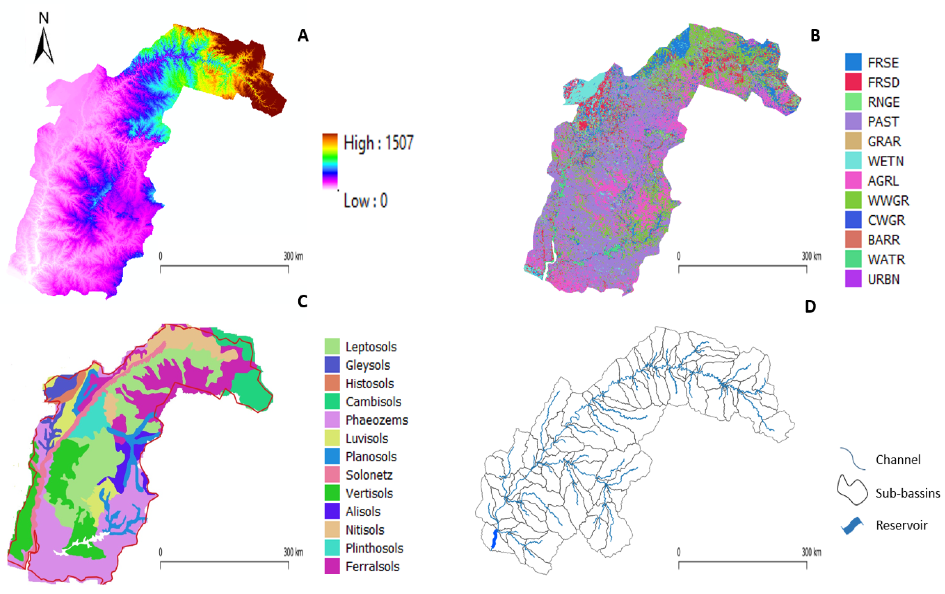
The required data to built a SWAT+ model include meteorological, hydrological, and physical variables. Figure 4 shows all the input data used for the model setup. During the watershed configuration process, sub-basins were subdivided into upland and floodplain areas.

2.5. Meteorological Data

Daily total precipitation data were acquired from the Climate Hazards group Infrared Precipitation with Stations (CHIRPSv2), with a spatial resolution of 0.25 degrees [27]. Maximum and minimum temperature and relative humidity daily data were obtained from the ERA5 reanalysis from the Copernicus Climate Change Service, with a spatial resolution of 0.5 degrees [28]. Wind speed and solar radiation were simulated using the weather generator integrated into SWAT+.

2.6. Topography

The Digital Elevation Map at 30 m resolution (DEM) was obtained from the shutter Radar Topography Mission, which is available from http://srtm.csi.cgiar.org/strmdata/ (accessed on 21 April 2021). Sub-basins and channel networks were obtained from this map.

2.7. Soil Data

The soil data were obtained from the Harmonized World Soil Database with the information contained within the 1:5,000,000 scale. Thirteen major soil groups were identified based on FAO/UNESCO-ISRIC classifications. Leptsols (shallow and stony soil) and ferrasols (red and yellow weathered soils with high concentrations of Al and Fe oxides) are predominant in the basin, and they comprise 26.75% and 9.83% of the total area, respectively.

2.8. Land Use Land Cover Data

Land Use and Land Cover data were obtained from the Copernicus Global Land Service (2019). Twelve land use types were identified according to SWAT+ classifications, in which pasture (PAST), western wheatgrass (WWGR), and agricultural land generic (WWGR) are the main classes, and occupy 35.49%, 18.09%, and 13.47% of the total area, respectively.

2.9. Model Set Up

The Uruguay River Basin was discretized into 221 sub-basins, 444 LSUs, and 4472 HRUs; the SWAT+ model setup covered approximately 215,000 km2. In addition, five categories of slope were defined; (1) flat (0–3%), (2) smooth (3–8%), (3) undulating (8–20%), (4) strongly undulating (20–45%), and (5) hilly (>45%). This slope classification was defined according to Embrapa (soil system classification of Brazil). For the calculation of evapotranspiration, the Hargreaves equation was chosen, and channel routing was calculated using the Muskingum routing method. SWAT+ uses the Soil Conversation Service Curve Number Method for runoff estimations [29]. The QGIS (v.3.22.5) QSWAT+ (v.60.5.4) interface was used to set up the model and run it at the daily time step, with a simulation period from 1987 to 2020 and three years of model warm-up.

2.10. River Discharge Data

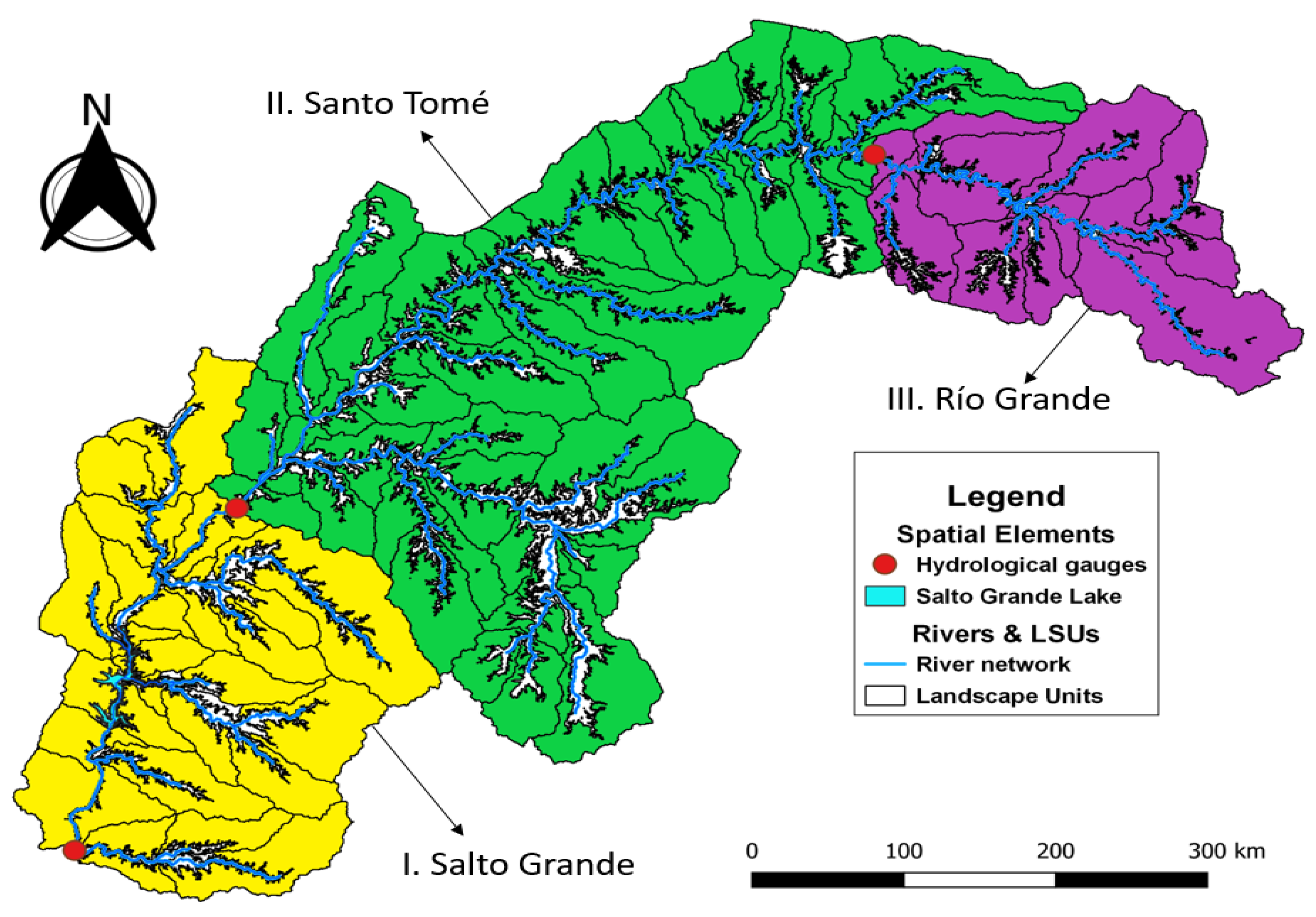
Daily streamflow data were obtained from the National Water Agency (ANA) of Brazil and from the Undersecretary of Water Resources in Argentina, and used for calibrating and validating the model. In this study, three stations located in the main river stream were calibrated. These cover the upper, mid, and low areas of the basin (Figure 5). We divided the Uruguay River Basin into three main areas in order to facilitate the discussion of results, these are (I) Salto Grande; (II) Santo Tomé; and (III) Río Grande. Table 1 shows the mean, standard deviation, median and asymmetry of the streamflow data for each hydrological station. The calibration and validation period varied according to the data availability of each station. The calibration and validation periods were, respectively:
I.
Salto Grande: from 1990 to 1997 and 1998 to 2001.
II.
Santo Tomé: from 1990 to 2010 and 2011 to 2020.
III.
Río Grande: from 1990 to 2000 and 2001 to 2010.

2.11. SPOTPY and Parameter Calibration

Parameter calibration and sensitivity and uncertainty analyses were performed using the SPOTPY open-source python library and it was linked with the SWAT+ model. SPOTPY has a model-independent structure, which means that can be easily linked to any eco-hydrological model. It contains eight commonly used algorithms and eleven objective functions, and can sample from eight parameter distributions [30].
In order to link SWAT+ to SPOTPY, three general applicable Python routines were developed. The first routine reads and modifies the parameter values used in the equations of SWAT+. The second routine reads the model outputs. Finally, the last routine reads the observed values, sets which parameters to calibrate and how to change them (whether absolute change, absolute value or percentage change), and defines the objective function(s) sample algorithm. For the calibration, we selected the Dream algorithm [31] and 3000 model runs. For the presented results herein, we show only the best performing model run, based on the calibrated likelihood function and quantify its performance with the NSE (Nash–Sutcliffe efficiency), KGE (Kling–Gupta efficiency), PBIAS (percent bias), and COR (correlation coefficient) objective functions. The underlying Python code is freely available at https://github.com/osvaluis/Spotswatplus (accessed on 21 April 2021).

2.12. Decision Table for Salto Grande Dam

SWAT+ allows the user to develop a set of rules (from simple to complex) to simulate reservoir release according to the variability of the volume of the reservoir. One main difficulty in developing a precise set of rules is the access to the management of the dam against flood and drought periods, ecological actions, and energy demands. In this study, we did not have access to Salto Grande dam data, and we developed the rules based on the available streamflow data. The dam of Salto Grande has two main uses: (1) energy production and (2) flood control. Thus, we extracted a decision table from the SWAT+ database for a dam that has approximately the same purpose and adjusted it to our case (Table 2). The structure, equations, and variables of the decision tables are explained in the work by Arnold et al. (2018) [18] and Wu et al. (2020) [32].
The decision table for the Salto Grande dam is interpreted as follows:
  • If reservoir volume > e-pv * −14.92, reservoir volume < e-pv * 0.005, and month < 5.86, then release volume for multiple_use_fl.
  • If reservoir volume > e-pv * −14.92, reservoir volume < e-pv * 0.005, and month > 10.06, then release volume for multiple_use_fl.
  • If reservoir volume > e-pv * −14.92, reservoir volume < e-pv * 0.005, month > 5.864, and month < 10.06, then release volume for multiple_use_nf.
  • If reservoir volume > e-pv * 0.005, reservoir volume < e-pv * 0.93, and month < 5.86, then release volume for sfl_cont+mu_fl.
  • If reservoir volume > e-pv * 0.005, reservoir volume < e-pv * 0.93, and month > 10.06, then release volume for sfl_cont+mu_fl.
  • If reservoir volume > e-pv * 0.005, reservoir volume < e-pv * 0.93, month > 5.86, and month < 10.06, then release volume for sfl_cont+mu_nf.
  • If reservoir volume > e-pv * 0.929, then release volume for efc_cont.

3. Results

3.1. Model Parameterization

The parameters perco (percolation coefficient), cn3_swf, and latq_co were first parameterized based on the Soil Vulnerability Index proposed by Tompson et al. (2020) [33]. The final values were assigned to each HRU classified as high, moderate, or low runoff and leaching potential based on the topography (slope of each HRU) and the hydrologic soil group. The calibrated parameters and their values are shown in Table 3.

3.2. Model Performance

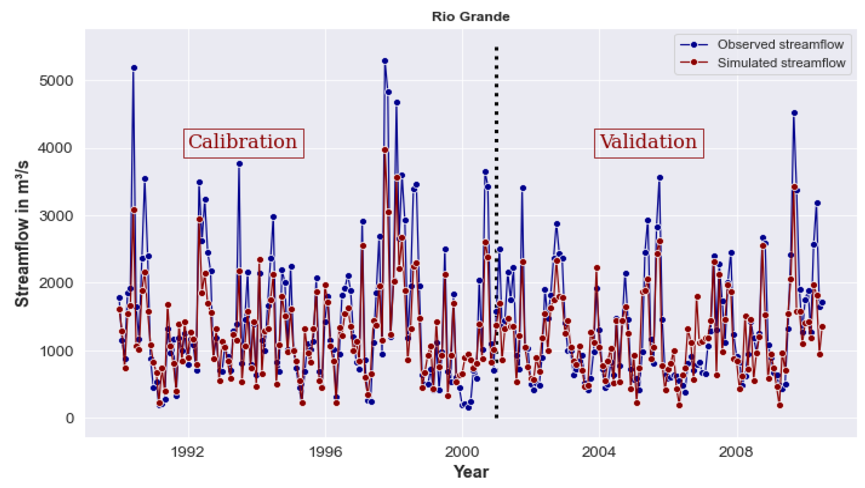
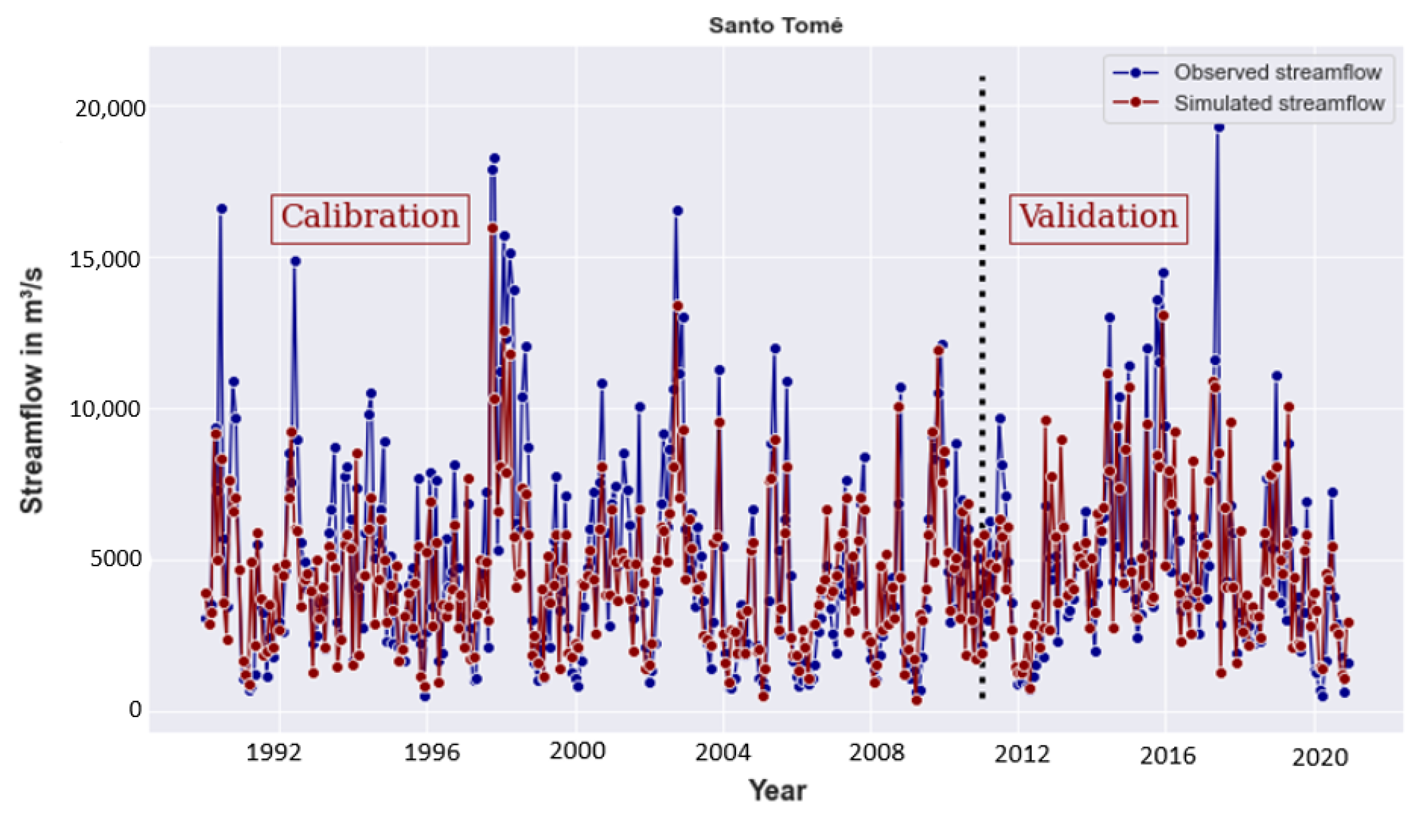
The model’s performance was analyzed on a monthly scale. Goodness-of-fit values for each region are shown in Table 4. The overall objective functions for both periods indicate a good performance on the model [34], while the model performs well for low flows, there is a general tendency to underestimate peak flows (Figure 6, Figure 7 and Figure 8).

3.3. Water Balance Components

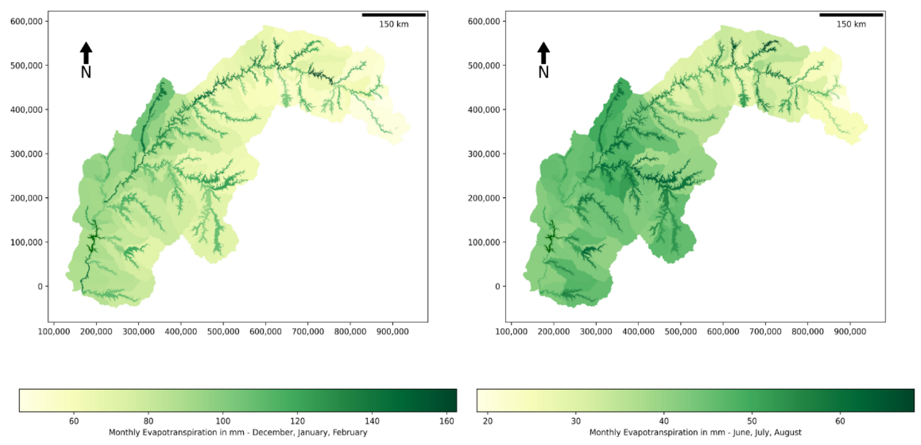
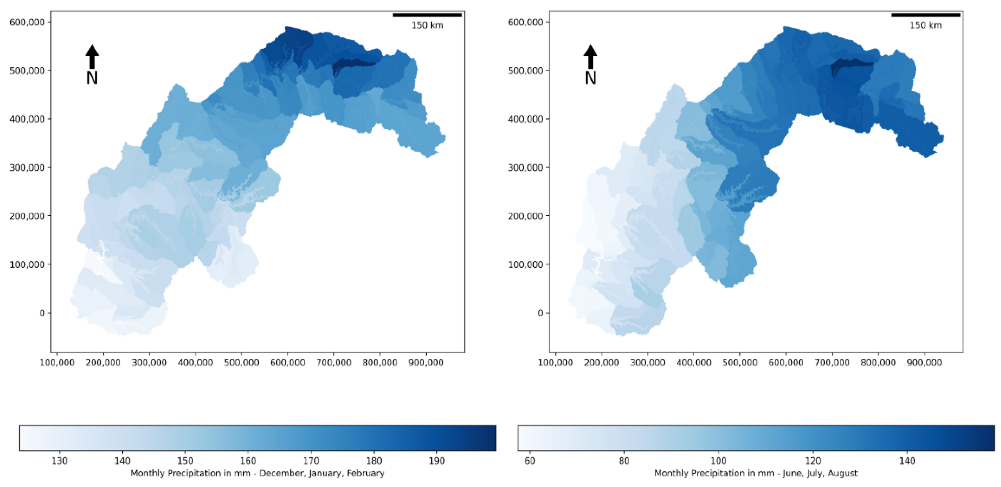
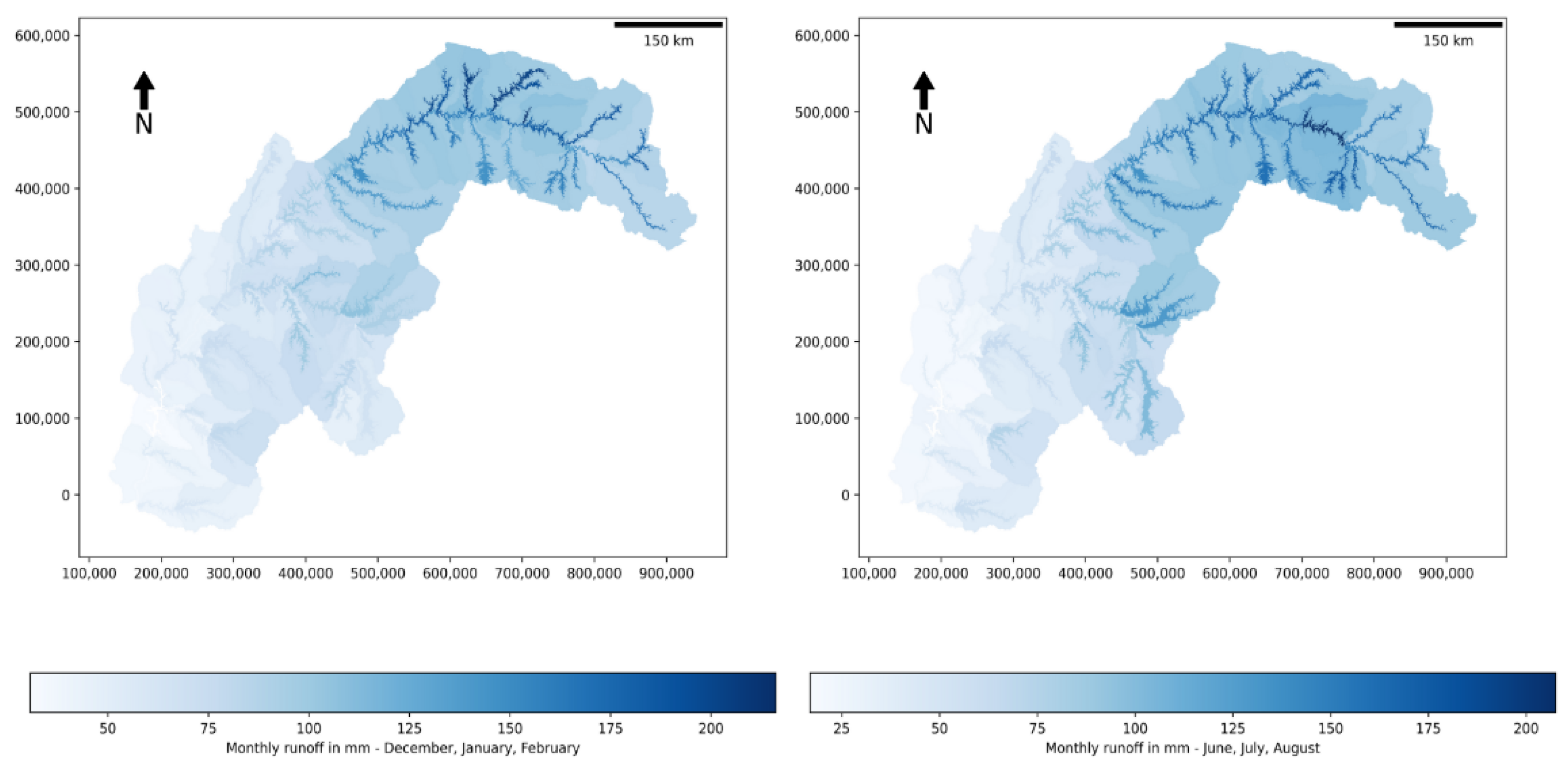
The final average annual amounts of the simulated water balance components are shown in Table 5. The spatial distributions for green and blue water are plotted for winter (June, July, and August) and summer periods (December, January, and February) in Figure 9, Figure 10, Figure 11 and Figure 12. Figure 9 and Figure 10 illustrate the seasonal soil water content and evapotranspiration in mm. The results indicate a higher content of water in floodplain areas. Figure 11 and Figure 12 show the spatial distribution of precipitation and surface runoff in mm. The upper URB receives more water from rainfall in both summer and winter periods. The total surface runoff generated from the landscape is also higher in the floodplain.

3.4. Observed and Simulated Data Evaluation

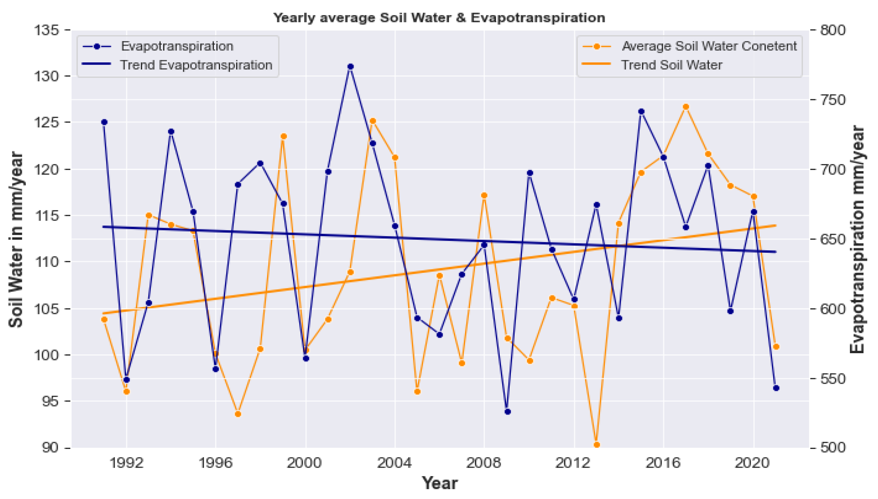
In order to analyze the variation of some hydro-meteorological components, thirty years of data were plotted within the period 1990–2020. Figure 13 illustrates the progression of precipitation, streamflow, and temperature. Figure 14 shows the evolution of ET and soil water content for the simulation period. A linear regression plot suggests a decrease in the annual evapotranspiration and an increase in the annual average temperature, precipitation, soil water content, and streamflow. In order to confirm these yearly variation trends, a Mann–Kendall seasonal test was performed using the pymannkendall python package [35].
The Mann–Kendall test showed a significant increasing trend for temperature (DJF), soil water content (JJA), and ET (DJF), with p-values of 0.007, 0.04, and 0.03, respectively (Table 6). No trends were identified for other water fluxes, such as precipitation and runoff.

4. Discussion

This study provides a detailed description of water fluxes and their principal trends in the Uruguay River Basin. One of the strengths of the current work is that the simulation was performed at a high spatial resolution, accounting for the upland and floodplain processes. In addition, this project was built for a long-term simulation over 30 years (1990–2020). These spatial and temporal resolutions were not found in previous studies of large-scale SWAT+ applications in the URB. For example, Tucci et al. (2003) [36] described a procedure for predicting seasonal flow in the Uruguay River Basin, but only modelled 75,000 km2 of the watershed. In addition, Guizzardi and Gerbec (2017) [37] applied the HEC-RAS model to calibrate and validate streamflow in only a five-year period.

4.1. Calibration and Validation Performance

The monthly simulations exhibited a range of performance levels from very good to satisfactory during both the calibration and validation periods, according to Moriasi et al. (2007) [34]. The upper and middle Basin area (Río Grande and Santo Tomé) provided the most accurate representation of the streamflow. However, the outlet zone showed the greatest underestimation, although it still had a satisfactory PBIAS. One potential reason of the model performance is the absence of marked seasonality in the streamflow regime in the URB [38]; consequently, there is a major difficulty for the model configuration in capturing the associated hydrological processes [39]. In addition, the inadequate knowledge of the Salto Grande reservoir management can lead to an insufficient representation of the release rates. Moreover, similar to SWAT, SWAT+ simulates two types of aquifers: shallow aquifer(s) that contribute to streamflow and deep or confined aquifers that account for the flow leaving the system. This simplistic representation of the groundwater-driven processes may lead to unrealistic base flow predictions in some model configurations, and therefore low NSE values [40,41]. Other sources of uncertainty may arise from the use of global reanalysis products that sometimes do not correctly resolve the atmosphere complexity [28]. Finally, the calibration procedure relies on achieving a good simulation of the actual physical processes in the URB. Therefore, we constrained the parameter sample space to obtain a realistic water balance, as recommended by Pfannerstill et al. (2017) [42].

4.2. Spatial Distribution of Water Fluxes

The water balance results indicate a good representation of the hydrological processes in the URB. The spatial distribution of the water balance components was performed at the LSU level. The addition of landscape units as a spatial discretization of the watershed allows a better representation of the hydrological components in the watershed [1,5,8,11,43]. The maximum ET and soil water content can be observed in the floodplain areas in both summer (DJF) and winter periods (JJA). This supports our hypothesis that the updated model structure results in a greater amount of water being available for ET and a higher soil water content in the lowlands (Figure 10 and Figure 11).
An increased surface runoff in the floodplain occurs because the runoff from the upland area is directed towards the floodplain, providing an additional source of input (Figure 13). The reduced values of lateral flow and percolation are attributable to specific characteristics of the river basin, namely (1) brief floods, (2) prompt reactions to precipitation, (3) soils with a low permeability and a shallow depth, and (4) a steep landscape [44]. Berbery and Barros studied the water cycle in the La Plata River Basin [24]. They hypothesized that the balance between precipitation, river discharge, evaporation, and infiltration are such that extreme interannual variability in precipitation is mostly translated to the river discharge and only a small fraction of it is converted in evapotranspiration or infiltration.
Differences in precipitation values in the uplands and floodplains can be explained by the spatial distribution of rainfall stations. SWAT+ reads the values of the nearest station to the HRU, and different stations do not have equal precipitation values. Figure 15 shows, for an upland–floodplain pair, the presence of at least six different rainfall stations.

4.3. Annual Variation in the Hydro-Meteorological Components during the Simulation Period (1990–2020)

An increase in the soil water content suggests that the URB can be considered as an atmospheric moisture sink. Su and Lettenmaier (2009) [38] also addressed this topic and concluded, through their estimation, that precipitation values exceed evapotranspiration levels in all seasons. A similar behavior, in a nearby geographical area, was reported by Collischonn et al. [45]. They observed an evapotranspiration increase over almost all the Parana river basin. This increase is related mostly to higher air temperatures and a potential precipitation increase. Even though there is a gradual warming over the URB (Figure 16), no trends were identified for other water fluxes, such as precipitation and runoff. One potential reason for this is the absence of regular patterns in precipitation regimes [24,38] in the river basin.

4.4. Limitations

The limitations of this model are mostly related in the data, i.e., (1) unavailability of reservoir management data and (2) no information on agricultural and management practices.
There are also limitations in the model configuration. For instance, for the SWAT+ revision used in this study, the connection between soils and aquifers is inaccurately represented; when the aquifer table is above the bottom of the soil, percolation from the soil is not limited, resulting in an underestimation of evapotranspiration and an unrealistic ground water flow.

5. Conclusions

The aim of this study was to represent the hydrological components across the Uruguay River Basin using the new version of the Soil and Water Assessment Tool (SWAT+) model. Furthermore, we analyzed hydro-meteorological trends using the large-scale built model.
The discretization of the watershed into LSUs results in a good representation of the spatial variability of the hydrological components. This is achieved through the quantification of upland and floodplain hydrological components, including runoff generated from the upland to the floodplain and lateral flow from the upland to the floodplain.
The goodness-of-fit results varied from very good to satisfactory at the three different gauges. The model performance at the outlet could be enhanced by providing an accurate decision table for the Salto Grande dam. A historical data analysis of different hydro-meteorological simulated variables indicated a significant increase in the average temperature (p-value = 0.007; Sen’s slope = 0.09), the soil water content (p-value = 0.02; Sen’s slope = 1.29), and evapotranspiration (p-value: 0.03; Sen’s slope = 1.97), indicating that the ecosystem experienced a changing climate during the simulation period.
The application of climate change models and the development of different scenario pathways can provide deeper insights into how climate change will affect water balance components in the catchment area.

Author Contributions

Conceptualization, O.L.B.A., S.S. and J.M.S.P.; methodology, O.L.B.A., K.B. and T.H.; software, O.L.B.A., K.B., C.S., T.H., S.S. and J.M.S.P.; validation, O.L.B.A., S.S. and J.M.S.P.; formal analysis, O.L.B.A., K.B., C.S., T.H., S.S. and J.M.S.P.; investigation, O.L.B.A., S.S. and J.M.S.P.; resources, O.L.B.A., S.S. and J.M.S.P.; data curation, O.L.B.A.; writing—original draft preparation, O.L.B.A., S.S. and J.M.S.P.; writing—review and editing, O.L.B.A., K.B., C.S., T.H., S.S. and J.M.S.P.; visualization, O.L.B.A., S.S. and J.M.S.P.; supervision, S.S. and J.M.S.P.; project administration, O.L.B.A.; funding acquisition, O.L.B.A., S.S. and J.M.S.P. All authors have read and agreed to the published version of the manuscript.

Funding

This study was partially supported through the grant EUR TESS N°ANR-18-EURE-0018 in the framework of the Programme des Investissements d’Avenir. The first author, Osvaldo Luis Barresi Armoa, is supported by the scholarship program Becas Don Carlos Antonio López (BECAL N°88/2021).

Data Availability Statement

Data are contained within the article.

Acknowledgments

The authors would like to acknowledge the technical support from Camargos, C. They also acknowledge the three anonymous reviewers whose helpful comments served to improve several parts of this article.

Conflicts of Interest

The authors declare no conflict of interest.

References

  1. Wagner, P.D.; Bieger, K.; Arnold, J.G.; Fohrer, N. Representation of hydrological processes in a rural lowland catchment in Northern Germany using SWAT and SWAT+. Hydrol. Process. 2022, 36, e14589. [Google Scholar] [CrossRef]
  2. Nkwasa, A.; Chawanda, C.J.; Van Griensven, A. Regionalization of the SWAT+ model for projecting climate change impacts on sediment yield: An application in the Nile basin. J. Hydrol. Reg. Stud. 2022, 42, 101152. [Google Scholar] [CrossRef] [PubMed]
  3. Jiménez-Navarro, I.C.; Jimeno-Sáez, P.; López-Ballesteros, A.; Pérez-Sánchez, J.; Senent-Aparicio, J. Impact of Climate Change on the Hydrology of the Forested Watershed That Drains to Lake Erken in Sweden: An Analysis Using SWAT+ and CMIP6 Scenarios. Forests 2021, 12, 1803. [Google Scholar] [CrossRef]
  4. Beven, K. Towards integrated environmental models of everywhere: Uncertainty, data and modelling as a learning process. Hydrol. Earth Syst. Sci. 2007, 11, 460–467. [Google Scholar] [CrossRef]
  5. Bieger, K.; Arnold, J.G.; Rathjens, H.; White, M.J.; Bosch, D.D.; Allen, P.M.; Volk, M.; Srinivasan, R. Introduction to SWAT+, a completely restructured version of the soil and water assessment tool. JAWRA J. Am. Water Resour. Assoc. 2017, 53, 115–130. [Google Scholar] [CrossRef]
  6. Chawanda, C.J.; Arnold, J.; Thiery, W.; van Griensven, A. Mass balance calibration and reservoir representations for large-scale hydrological impact studies using SWAT+. Clim. Chang. 2020, 163, 1307–1327. [Google Scholar] [CrossRef]
  7. Bailey, R.T.; Bieger, K.; Arnold, J.G.; Bosch, D.D. A new physically-based spatially-distributed groundwater flow module for SWAT+. Hydrology 2020, 7, 75. [Google Scholar] [CrossRef]
  8. Bieger, K.; Arnold, J.G.; Rathjens, H.; White, M.J.; Bosch, D.D.; Allen, P.M. Representing the connectivity of upland areas to floodplains and streams in SWAT+. JAWRA J. Am. Water Resour. Assoc. 2019, 55, 578–590. [Google Scholar] [CrossRef]
  9. Kiprotich, P.; Wei, X.; Zhang, Z.; Ngigi, T.; Qiu, F.; Wang, L. Assessing the impact of land use and climate change on surface runoff response using gridded observations and swat+. Hydrology 2021, 8, 48. [Google Scholar] [CrossRef]
  10. Abate, B.Z.; Assefa, T.T.; Tigabu, T.B.; Abebe, W.B.; He, L. Hydrological Modeling of the Kobo-Golina River in the Data-Scarce Upper Danakil Basin, Ethiopia. Sustainability 2023, 15, 3337. [Google Scholar] [CrossRef]
  11. Pulighe, G.; Lupia, F.; Chen, H.; Yin, H. Modeling climate change impacts on water balance of a Mediterranean watershed using SWAT+. Hydrology 2021, 8, 157. [Google Scholar] [CrossRef]
  12. Eini, M.R.; Salmani, H.; Piniewski, M. Comparison of process-based and statistical approaches for simulation and projections of rainfed crop yields. Agric. Water Manag. 2023, 277, 108107. [Google Scholar] [CrossRef]
  13. Eini, M.R.; Massari, C.; Piniewski, M. Satellite-based soil moisture enhances the reliability of agro-hydrological modeling in large transboundary river basins. Sci. Total Environ. 2023, 873, 162396. [Google Scholar] [CrossRef] [PubMed]
  14. Tan, M.L.; Juneng, L.; Kuswanto, H.; Do, H.X.; Zhang, F. Impacts of Solar Radiation Management on Hydro-Climatic Extremes in Southeast Asia. Water 2023, 15, 1089. [Google Scholar] [CrossRef]
  15. Xiao, F.; Wang, X.; Fu, C. Impacts of land use/land cover and climate change on hydrological cycle in the Xiaoxingkai Lake Basin. J. Hydrol. Reg. Stud. 2023, 47, 101422. [Google Scholar] [CrossRef]
  16. Hordofa, A.T.; Leta, O.T.; Alamirew, T.; Chukalla, A.D. Climate Change Impacts on Blue and Green Water of Meki River Sub-Basin. Water Resour. Manag. 2023, 37, 2835–2851. [Google Scholar] [CrossRef]
  17. Chawanda, C.J.; George, C.; Thiery, W.; Van Griensven, A.; Tech, J.; Arnold, J.; Srinivasan, R. User-friendly workflows for catchment modelling: Towards reproducible SWAT+ model studies. Environ. Model. Softw. 2020, 134, 104812. [Google Scholar] [CrossRef]
  18. Arnold, J.G.; Bieger, K.; White, M.J.; Srinivasan, R.; Dunbar, J.A.; Allen, P.M. Use of decision tables to simulate management in SWAT+. Water 2018, 10, 713. [Google Scholar] [CrossRef] [Green Version]
  19. Bailey, R.T.; Abbas, S.; Arnold, J.; White, M.; Gao, J.; Čerkasova, N. Augmenting the National agroecosystem model with physically based spatially distributed groundwater modeling. Environ. Model. Softw. 2023, 160, 105589. [Google Scholar] [CrossRef]
  20. Yimer, E.A.; Bailey, R.T.; Piepers, L.L.; Nossent, J.; van Griensven, A. Improved representation of groundwater-dominated catchment using SWAT+ gwflow and modifications to the gwflow module. Hydrol. Earth Syst. Sci. Discuss. 2022, 1–18. [Google Scholar] [CrossRef]
  21. Yimer, E.A.; Riakhi, F.E.; Bailey, R.T.; Nossent, J.; van Griensven, A. The impact of extensive agricultural water drainage on the hydrology of the Kleine Nete watershed, Belgium. Sci. Total Environ. 2023, 885, 163903. [Google Scholar] [CrossRef]
  22. Rockström, J. On-farm green water estimates as a tool for increased food production in water scarce regions. Phys. Chem. Earth Part D Hydrol. Ocean. Atmos. 1999, 24, 375–383. [Google Scholar] [CrossRef]
  23. Saurral, R.I.; Barros, V.R.; Lettenmaier, D.P. Land use impact on the Uruguay River discharge. Geophys. Res. Lett. 2008, 35, 12. [Google Scholar] [CrossRef]
  24. Berbery, E.H.; Barros, V.R. The hydrologic cycle of the La Plata basin in South America. J. Hydrometeorol. 2002, 3, 630–645. [Google Scholar] [CrossRef]
  25. Tossini, L. Sistema hidrográfico y cuenca del Río de la Plata: Contribución al estudio de su régimen hidrológico. Anales Sociedad Científica Argentina 1959, 167, 41–64. [Google Scholar]
  26. Arnold, J.G.; Srinivasan, R.; Muttiah, R.S.; Williams, J.R. Large area hydrologic modeling and assessment part I: Model development 1. JAWRA J. Am. Water Resour. Assoc. 1998, 34, 73–89. [Google Scholar] [CrossRef]
  27. Funk, C.; Peterson, P.; Landsfeld, M.; Pedreros, D.; Verdin, J.; Shukla, S.; Husak, G.; Rowland, J.; Harrison, L.; Hoell, A.; et al. The climate hazards infrared precipitation with stations—A new environmental record for monitoring extremes. Sci. Data 2015, 2, 1–21. [Google Scholar] [CrossRef] [Green Version]
  28. Hersbach, H.; Bell, B.; Berrisford, P.; Hirahara, S.; Horányi, A.; Muñoz-Sabater, J.; Nicolas, J.; Peubey, C.; Radu, R.; Schepers, D.; et al. The ERA5 global reanalysis. Q. J. R. Meteorol. Soc. 2020, 146, 1999–2049. [Google Scholar] [CrossRef]
  29. Slack, R.; Welch, R. Soil conservation service runoff curve number estimates from landsat data 1. JAWRA J. Am. Water Resour. Assoc. 1980, 16, 887–893. [Google Scholar] [CrossRef]
  30. Houska, T.; Kraft, P.; Chamorro-Chavez, A.; Breuer, L. SPOTting model parameters using a ready-made python package. PLoS ONE 2015, 10, e0145180. [Google Scholar] [CrossRef] [Green Version]
  31. Vrugt, J.A. Markov chain Monte Carlo simulation using the DREAM software package: Theory, concepts, and MATLAB implementation. Environ. Model. Softw. 2016, 75, 273–316. [Google Scholar] [CrossRef] [Green Version]
  32. Wu, J.; Yen, H.; Arnold, J.G.; Yang, Y.E.; Cai, X.; White, M.J.; Santhi, C.; Miao, C.; Srinivasan, R. Development of reservoir operation functions in SWAT+ for national environmental assessments. J. Hydrol. 2020, 583, 124556. [Google Scholar] [CrossRef]
  33. Thompson, A.; Baffaut, C.; Lohani, S.; Duriancik, L.; Norfleet, M.; Ingram, K. Purpose, development, and synthesis of the Soil Vulnerability Index for inherent vulnerability classification of cropland soils. J. Soil Water Conserv. 2020, 75, 1–11. [Google Scholar] [CrossRef] [Green Version]
  34. Moriasi, D.N.; Arnold, J.G.; Van Liew, M.W.; Bingner, R.L.; Harmel, R.D.; Veith, T.L. Model evaluation guidelines for systematic quantification of accuracy in watershed simulations. Trans. ASABE 2007, 50, 885–900. [Google Scholar] [CrossRef]
  35. Hussain, M.; Mahmud, I. pyMannKendall: A python package for non parametric Mann Kendall family of trend tests. J. Open Source Softw. 2019, 4, 1556. [Google Scholar] [CrossRef]
  36. Tucci, C.E.M.; Clarke, R.T.; Collischonn, W.; da Silva Dias, P.L.; de Oliveira, G.S. Long-term flow forecasts based on climate and hydrologic modeling: Uruguay River basin. Water Resour. Res. 2003, 39, 7. [Google Scholar] [CrossRef] [Green Version]
  37. Guizzardi, S.; Gerbec, M.S. Modelación Hidrológica e Hidrodinámica del Río Uruguay. In Proceedings of the Conagua 2017, Córdoba, Argentina, 20–23 September 2017. [Google Scholar]
  38. Su, F.; Lettenmaier, D.P. Estimation of the surface water budget of the La Plata Basin. J. Hydrometeorol. 2009, 10, 981–998. [Google Scholar] [CrossRef]
  39. Gudmundsson, L.; Wagener, T.; Tallaksen, L.; Engeland, K. Evaluation of nine large-scale hydrological models with respect to the seasonal runoff climatology in Europe. Water Resour. Res. 2012, 48, 11. [Google Scholar] [CrossRef]
  40. Srivastava, P.; McNair, J.N.; Johnson, T.E. Comparison of process-based and artificial neural network approaches for streamflow modeling in an agricultural watershed. JAWRA J. Am. Water Resour. Assoc. 2006, 42, 545–563. [Google Scholar] [CrossRef]
  41. Wu, K.; Johnston, C.A. Hydrologic response to climatic variability in a Great Lakes Watershed: A case study with the SWAT model. J. Hydrol. 2007, 337, 187–199. [Google Scholar] [CrossRef]
  42. Pfannerstill, M.; Bieger, K.; Guse, B.; Bosch, D.D.; Fohrer, N.; Arnold, J.G. How to constrain multi-objective calibrations of the SWAT model using water balance components. JAWRA J. Am. Water Resour. Assoc. 2017, 53, 532–546. [Google Scholar] [CrossRef]
  43. Nkwasa, A.; Chawanda, C.J.; Jägermeyr, J.; Van Griensven, A. Improved representation of agricultural land use and crop management for large-scale hydrological impact simulation in Africa using SWAT+. Hydrol. Earth Syst. Sci. 2022, 26, 71–89. [Google Scholar] [CrossRef]
  44. Míguez, D. Breve reseña sobre el Río Uruguay. INNOTEC 2007, 2, 7–9. [Google Scholar]
  45. Metcalfe, C.D.; Collins, P.; Menone, M.L.; Tundisi, J.G. The Paraná River Basin: Managing Water Resources to Sustain Ecosystem Services; Routledge: London, UK, 2020. [Google Scholar]
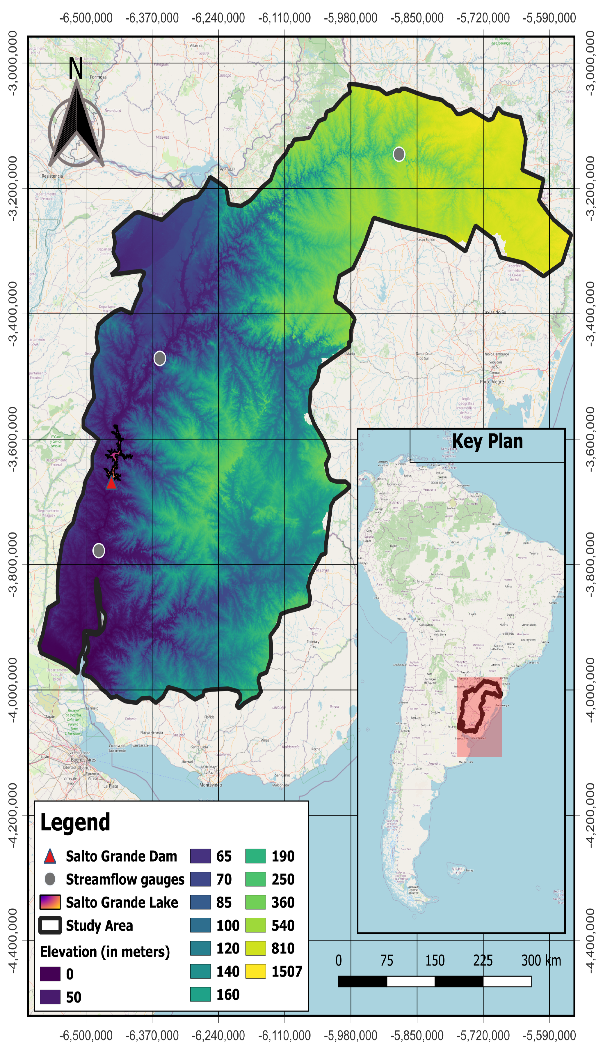
Figure 1. Topography map of the study area of the Uruguay River Basin (URB), with a catchment size of 370,000 km² and an elevation ranging from 0 to 1500 m above sea level, located in South America.
Water 15 02604 g001
Figure 2. Monthly temperature in degrees Celsius based on the ERA5 dataset. The color palette indicates the increase in temperature between months. Isotherm values are approximately between 16 and 24 degrees.
Water 15 02604 g002
Figure 3. Connectivity representation in SWAT+. AQU, aquifer; LSU, landscape unit; HRU, hydrologic response unit. Different colors represent different hydrological components in the sub-basin.
Water 15 02604 g003
Figure 4. Maps of (A) topography (in meters), (B) land use and land cover, (C) soil type, (D) channel network and sub-basins of the Uruguay River Basin. FRSE: forest—evergreen, FRSD: forest—deciduous, RNGE: range—grasses, PAST: pasture, GRAR: grarigue, WETN: wetlands non-forested, AGRL: agricultural land—generic, WWGR: western wheatgrass, CWGR: crested wheatgrass, BARR: barren, WATR: water, URBN: residential.
Water 15 02604 g004
Figure 5. Uruguay River Basin with its sub-basins showing the spatial distribution of the hydrological stations. I. Salto Grande (low URB), II. Santo Tomé (mid URB), III. Río Grande (upper URB).
Water 15 02604 g005
Figure 6. Río Grande (upper Uruguay Basin). Comparison between observed and simulated values from 1990 to 2010. Calibration period: NSE 0.77; PBIAS −7.61; COR 0.93; KGE 0.63. Validation period: NSE 0.70; PBIAS −5.59; COR 0.86; KGE 0.65.
Water 15 02604 g006
Figure 7. Santo Tomé (middle Uruguay Basin). Comparison between observed and simulated values from 1990 to 2020. Calibration period: NSE 0.65; PBIAS −17.02; COR 0.88; KGE 0.60. Validation period: NSE 0.62; PBIAS −7.05; COR 0.80; KGE 0.68.
Water 15 02604 g007
Figure 8. Salto Grande (lower Uruguay Basin). Comparison between observed and simulated values from 1990 to 2001. Calibration period: NSE 0.62; PBIAS −22.01; COR 0.89; KGE 0.60. Validation period: NSE 0.63, PBIAS −24.73; COR 0.92; KGE 0.60.
Water 15 02604 g008
Figure 9. Monthly mean of the soil water content in mm for June, July, and August and December, January, and February (1990–2020).
Water 15 02604 g009
Figure 10. Monthly mean evapotranspiration from the soil in mm for June, July, and August and December, January, and February (1990–2020).
Water 15 02604 g010
Figure 11. Monthly mean precipitation in mm for June, July, and August and December, January, and February (1990–2020).
Water 15 02604 g011
Figure 12. Monthly mean runoff in mm for June, July, and August and December, January, and February (1990–2020).
Water 15 02604 g012
Figure 13. Yearly average precipitation and simulated streamflow in mm and temperature in Celsius degrees with their linear regression curves.
Water 15 02604 g013
Figure 14. Yearly average soil water content and evapotranspiration in mm with their respective linear regression curves.
Water 15 02604 g014
Figure 15. Spatial distribution of precipitation stations over the watershed. For the upland–floodplain pair there are at least six different rainfall stations.
Water 15 02604 g015
Figure 16. Annual mean maximum and minimum temperature in the URB.
Water 15 02604 g016
Table 1. Mean, standard deviation, median (in m3/s), and asymmetry coefficient of the observed monthly streamflow.
GaugeMeanStandard DeviationMedianAsymmetry
Salto Grande6213.173830.185220.491.26
Santo Tomé4949.863444.334153.011.33
Río Grande1410.01982.491104.181.39
Table 2. Decision table for the Salto Grande dam. Conditions (conds); alternatives (alts); limit variable (lim_var); limit operator (lim_op); limit constant (lim_const); file pointer (fp); storage volume in ha-m (e-pv); day rate (dyrt). Multiple use flood (multiple_use_fl); multiple use non-flood (multiple_use_nf); seasonal flood control + multiple use flood (sfl_cont+mu_fl); seasonal flood control + multiple use non-flood (sfl_cont+mu_nf); emergency flood control (efc_cont).
Name Conds Alts Acts
Salto 5 7 5
Variable Object lim_var lim_oplim_constalt1alt2alt3alt4alt5alt6alt7
volumerese-pv*−14.92>>>----
volumerese-pv*0.005<<<>>>-
volumerese-pv*0.93---<<<>
monthnullnull*5.86<-><->-
monthnullnull*10.06-><-><-
Action ObjectNameOptionConstantConstant 2fpOutcome
releaseresmultiple_use_fldyrt1950.17con1y y n n n n n
releaseresmultiple_use_nfdyrt450.29con1n n y n n n n
releaseressfl_cont+mu_fldyrt153.00con2n n n y y n n
releaseressfl_cont+mu_nfdyrt254.93con2n n n n n y n
releaseresefc_contdyrt55.16con3n n n n n n y
Table 3. Initial boundaries and final calibrated values of each investigated SWAT+ model parameter. Absolute value (absval); absolute change (abschg).
ParameterDescriptionMinMaxChangeFinal Value
flo_minThreshold required for return flow to occur (meters)1015absval10.03
alphaBaseflow recession constant (days)0.012.0absval1.97
sp_yldRatio of the volume of water drained by gravity (fraction)0.100.20absval0.15
escoSoil evaporation coefficient01absval0.99
epcoPlant uptake coefficient01absval0.90
awcAvailable water capacity of the soil layer (mm H2O/mm)−0.09−0.30abschg−0.24
cn3_swfSoil water factor for the curve number condition III−0.30−0.10abschg−0.25
cn2Curve number condition II0.050.15abschg0.10
canmxMaximum canopy storage (mm H2O)−0.10−0.35abschg−0.29
chwChannel width (meters)−0.10−0.30abschg−0.15
kSaturated hydraulic conductivity (mm/h)−0.1−0.7abschg−0.49
bf_maxBaseflow rate (mm)0.12.0absval1.98
surlagSurface runoff lag coefficient0.90.1abschg0.50
Table 4. Objective function values for calibration and validation periods on a monthly time scale. Nash–Sutcliffe model efficiency (NSE); percent bias (PBIAS); correlation coefficient (COR); Kling–Gupta efficiency (KGE).
Calibration
Objective FunctionSalto GrandeSanto ToméRio Grande
NSE0.620.650.77
PBIAS−22.01−17.02−7.61
COR0.890.880.93
KGE0.600.600.63
Validation
NSE0.630.620.70
PBIAS−24.73−7.05−5.59
COR0.920.800.86
KGE0.600.680.65
Table 5. Mean annual water balance components for the Uruguay River Basin in mm.
VariableDescriptionValue
pcpPrecipitation1689.13
ETEvapotranspiration739.73
s u r q g e n Runoff generated from the landscape933.64
s u r q r u n o n Runoff from upland to the floodplain83.81
latqLat. flow from landscape38.83
l a t q r u n o n Lat. flow from upland to the floodplain34.30
percoPercolation91.86
wateryldWater yield972.47
Obs *Observed flow at Salto Grande (outlet)990.34
* Undersecretary of Water Resources in Argentina (Concepcion gauge).
Table 6. Annual variability analysis for meteorological and hydrological components from 1990 to 2020. Mann–Kendall seasonal test (significance level 0.05) and Sen’s slope ( β > 0 increasing trend and β < 0 decreasing trend). Average temperature (Avg. Temp), evapotranspiration (ET), precipitation, runoff, and soil water content (soil water) for December–January–February (DJF) and June–July–August (JJA).
VariableZ (Trend)p-ValueSen’s Slope
Precipitation DJFno trend0.373.90
Precipitaion JJAno trend0.651.11
Avg. Temp DJFincreasing0.0070.09
Avg. Temp JJAno trend0.880.03
Runoff DJFno trend0.262.72
Runoff JJAno trend0.940.47
ET DJFincreasing0.031.97
ET JJAno trend0.160.37
Soil Water DJFno trend0.081.09
Soil Water JJAincreasing0.041.13
Disclaimer/Publisher’s Note: The statements, opinions and data contained in all publications are solely those of the individual author(s) and contributor(s) and not of MDPI and/or the editor(s). MDPI and/or the editor(s) disclaim responsibility for any injury to people or property resulting from any ideas, methods, instructions or products referred to in the content.