Article

Analysis and Exploration of the Impact of Average Sea Level Change on Navigational Safety in Ports

1
Department of Navigation, Taipei University of Marine Technology, Taipei 11174, Taiwan
2
Department of Shipping Technology, National Kaohsiung University of Science and Technology, Kaohsiung 805301, Taiwan
*
Author to whom correspondence should be addressed.
Water 2023, 15(14), 2570; https://doi.org/10.3390/w15142570
Submission received: 13 June 2023 / Revised: 10 July 2023 / Accepted: 12 July 2023 / Published: 13 July 2023
(This article belongs to the Special Issue Advanced Research in Civil, Hydraulic, and Ocean Engineering)

Abstract

:
The primary clientele of a harbor is vessels, and vessels are primarily influenced by external forces such as wind (on the water surface), currents (underwater), and waves (affecting vessel stability). Therefore, it is necessary to comprehensively consider safety factors such as marine environmental forces and port characteristics. As ship sailing falls under applied science, acquiring marine meteorological information regarding ship routes can enhance port navigational safety. However, in the face of changes in the environmental conditions of harbor waters, it is essential to fully consider the impact of the external environment on ship maneuvering. One can effectively navigate complex operating environments by devising reasonable ship-handling plans. In the context of sea level rise caused by extreme climatic events, long-term variations, trends, and random factors are at play. Previous assessments of sea level rise have often relied on linear regression and the least squares method to determine coefficients. However, these methods fail to accurately capture the actual trend of sea level rise. Additionally, traditional harmonic analysis methods are unable to analyze sea level rise as well. Therefore, in this study, the techniques of simple moving average (SMA), empirical mode decomposition (EMD), and ensemble empirical mode decomposition (EEMD) were applied to analyze sea level rise. The obtained results of sea level rise under different analysis conditions were integrated with a hydrodynamic model that incorporates both wave and tidal characteristics to calculate the overall coastal dynamics parameters, which are crucial for ship navigation. The research findings contribute to the study of ship navigational safety issues by examining the distribution characteristics of port meteorology under climate change conditions. They offer valuable insights for mariners to assess navigational safety and devise maneuvering strategies based on the actual water flow conditions. Furthermore, the findings help identify and address potential risks and issues, ultimately ensuring the safety of navigation.

1. Introduction

Ports are the foundation for maritime engineering development and are the hub for sea and land transportation. More than 90% of global trade is conducted through maritime shipping. The effectiveness of port construction relies on ensuring the safe navigation of ships during entry, safe navigation within port waters, and secure mooring and loading/unloading operations. Over time, ship designs have evolved toward larger sizes to meet the advancements in shipbuilding technology and the demands of maritime transportation. The water area between the outer channel and the breakwater entrance of the harbor is primarily influenced by environmental factors such as wind and currents. Safety considerations in this area require a comprehensive assessment of ship handling, environmental forces, and port characteristics. Evaluating the safety of entering the port relies on considering these factors. Therefore, the requirements of a port are closely related to climate conditions.
Climate change issues related to global warming have become increasingly prominent in recent years. One of the critical concerns is the rise in sea levels, along with other environmental changes. Research on sea level rise [1,2,3,4,5,6] indicates that the global mean sea level has been rising at approximately 1.5 to 2.4 mm per year during the 20th century. According to the final draft of the Working Group I contribution to the Intergovernmental Panel on Climate Change (IPCC) Sixth Assessment Report (AR6) released on 9 August 2021 [7], observations of extreme weather and climate events since 1950 have shown an increase in the frequency and duration of warm periods, rainfall intensity, intense tropical cyclone activity, and the likelihood of extreme high sea levels. The report also states that from 1901 to 2018, the global mean sea level has risen by 200 mm, with a rate of 1.3 mm per year from 1901 to 1971, 1.9 mm per year from 1971 to 2006, and an increase of 3.7 mm per year from 2006 to 2018. Climate change has significantly impacted most terrestrial and marine areas worldwide. Changes in hydrological conditions, for example, directly affect the characteristics of coastal environments and can even impact the functionality of coastal protection structures and port operations. Due to global climate change, there has been a rise in average sea levels, leading to changes in local hydrodynamic features such as tides, waves, and currents in coastal areas. Considering the safety of vessel navigation, it is primarily influenced by environmental factors such as wind and currents. It is essential to effectively understand the dynamics of tides, waves, and currents in the vicinity of ports and the distribution characteristics of nearshore flow fields influenced by the water depth and topography near the ports. Therefore, studying tidal and sea level variations holds significant importance and practical value [8,9,10,11,12,13,14].
Keelung Port is an important harbor in northern Taiwan. During the era of economic takeoff, it played a crucial role as the country’s artery for international trade and cargo transportation. Container shipping is the primary mode of transportation, supplemented by bulk cargo. In December 2009, the largest cargo vessel to ever dock in the port, the MSC MARIA ELENA, arrived. The MSC MARIA ELENA had a capacity of 9100 TEUs (TEU: twenty-foot equivalent unit), with a length of 336 m, a width of 45.6 m, and a maximum draft of 14 m. In recent years, with the government actively promoting the transformation of Keelung Port into a tourism and recreational harbor, it has become Taiwan’s primary international cruise port. In May 2023, the port welcomed the MSC Bellissima cruise ship, with a total tonnage of 172,000 tons (length: 315.83 m, width: 43 m, draft: 8.75 m), setting a record as the largest cruise ship to dock at Keelung Port. However, due to their significant inertia and small length-to-width ratio, large vessels require the careful consideration of ship-handling characteristics, environmental forces, and port characteristics when maneuvering to assess their safety during port entry [15,16,17,18,19,20,21,22,23].
Due to the influence of coastal dynamics factors such as tides, waves, currents, and topography, the distribution of water flow near port channels is affected. Considering the rising sea levels caused by global warming, there is concern that it may alter the characteristics of tidal patterns, waves, and currents in the marine environment. Among these external conditions, the selection of basic flow field parameters is crucial for vessel navigation, as the flow distribution can be affected by changes in port structures and topography, resulting in more complex flow conditions in port areas [24,25,26,27]. In general, when the direction of water flow is not aligned with the ship’s heading, the flowing water exerts a hydrodynamic pressure on the vessel. The impact on the ship becomes more significant as the angle between the flow direction and the ship’s heading increases.
Furthermore, as the ship moves, the effects of the water flow on the vessel shift gradually from the bow to the stern [28,29,30]. To ensure navigation safety, the assessment of the safety impact on ship navigation during port entry and exit is often conducted using computer simulations. Therefore, this study employed a harmonization analysis framework to investigate coastal tidal characteristics and sea level trends. The analysis involved the application of simple moving average (SMA), empirical mode decomposition (EMD), and ensemble empirical mode decomposition (EEMD) to analyze sea level rise. Next, the obtained results of a sea-level-rise analysis will be validated using a numerical model considering wave–flow interactions, with field observations as background data. This study investigates the impact of port sea–meteorological distribution characteristics on ship navigation safety under climate change conditions. The analysis results will provide navigation personnel with a safety assessment and maneuvering strategy considering the actual distribution of water currents. Additionally, it can serve as a reference for maritime and relevant authorities in ensuring navigation safety in the fairway.

2. Sea-Level-Rise Analysis

2.1. Analysis of Water Level Data

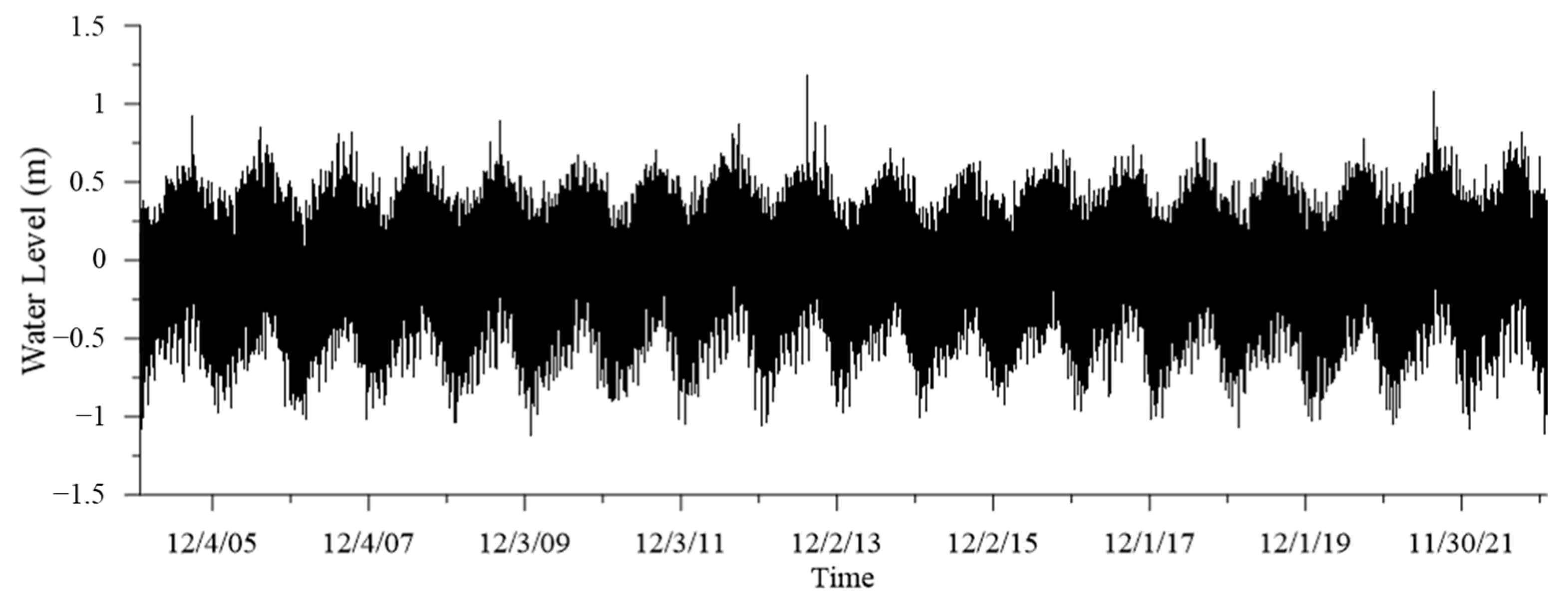
This study selected the location of the tide gauge station at Keelung Port, as shown in Figure 1 (25.155° N, 121.7522° E). However, the instrument’s position may change due to human factors such as maintenance or natural disasters like typhoons, which can result in instrument damage or the cessation of recording. These factors can affect the integrity of the actual tide data. The statistical analysis of hourly water level data, as shown in Figure 2, indicates that the completeness of the tidal data at the Keelung Port tide gauge station from 2005 to 2022 is approximately 88.9%. To compensate for the data gaps, the measured data were subjected to harmonic analysis, and the missing astronomical tide data were filled in at the gaps in the original data. The missing tidal data in the original dataset were filled with predicted astronomical tide data, as shown in Figure 3. Subsequently, three different methods, namely SMA, EMD, and EEMD, were applied separately to analyze the sea level rise at Keelung Port.

2.2. Methods for Analyzing Sea Level

In this study, the harmonic analysis framework was utilized to analyze sea level rise using three different methods: SMA, EMD, and EEMD. Moving average (MA) aims to smooth out data fluctuations by taking the average, making the trend of the data more apparent. MAs can be categorized into three methods: simple moving average (SMA), weighted moving average (WMA), and exponential moving average (EMA), depending on the calculation method. WMA and EMA assign weights to data from different periods based on the SMA. The weights are higher for data closer to the current period, indicating a more significant impact on the average. In simple terms, WMA and EMA are more responsive to recent data changes. However, the SMA is still the most commonly used method, especially in various technical indicators and analyses. The formula for calculating the SMA is as follows:
F t + 1 = D t + D t 1 + D t 2 + + D t n + 1 n
where F t + 1 represents the forecast value for the next period, n denotes the number of periods for the moving average, and D t , D t 1 , D t 2 , and D t n + 1 represent the data for the previous period, two periods ago, three periods ago, and up to n periods ago, respectively.
This study applied the SMA to analyze the tidal water level data from the Keelung tide gauge station from 2005 to 2022. The moving average was calculated over one year, resulting in the Keelung tidal water level trend line shown in Figure 4. The estimated rise in sea level is approximately 17.68 mm, with an average sea-level-rise rate of 0.98 mm/yr.
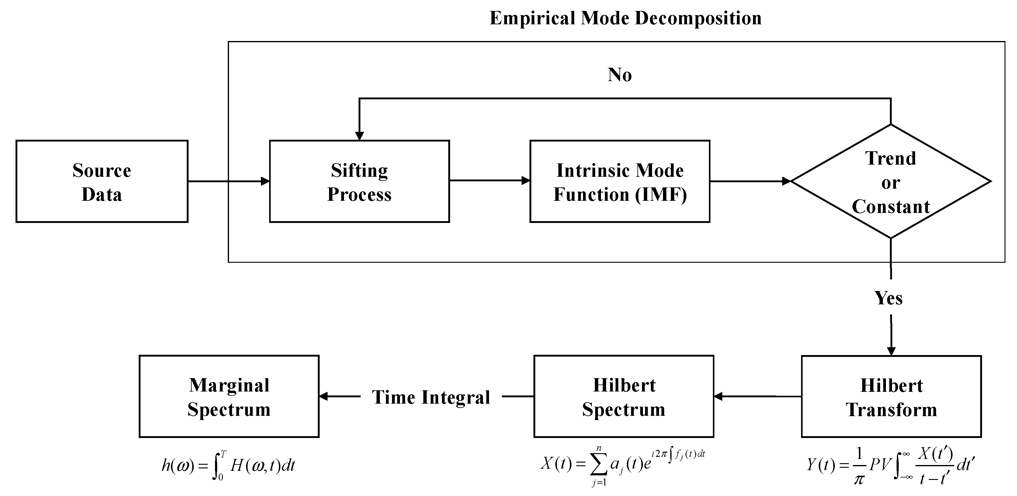
Next, this study applies the Hilbert–Huang transform (HHT), which consists of empirical mode decomposition (EMD) and Hilbert transform (HT), for analysis. The HHT can analyze non-stationary and non-linear data, making it applicable in various fields such as seismic signal analysis, the detection of damage in bridges or highway structures, the processing of biomedical signals, and the measurement of tides or waves. The common characteristic of these applications is that they can be presented in frequency form, and the input signals are often non-stationary data [31]. HHT decomposes a signal into multiple components called intrinsic mode functions (IMFs). These IMF components are not necessarily complete and symmetrical sinusoids. Their periods and amplitudes are not fixed, allowing for meaningful instantaneous frequency and instantaneous amplitude to be directly obtained using the Hilbert transform (HT). HHT exhibits physical significance, high precision, and adaptability. The empirical mode decomposition (EMD) in HHT refers to decomposing a signal into multiple IMF components. This process requires multiple iterations to obtain each IMF. The procedure is as follows.
The original signal s t is inputted, and all local maxima and local minima are identified. Then, curve fitting is performed on all the local maxima and local minima. Cubic spline interpolation is commonly used for curve fitting in HHT. Cubic spline interpolation provides results closest to the actual curve compared to other interpolation methods. After the interpolation is completed, upper and lower envelopes are obtained separately. Then, the average of the upper and lower envelopes is calculated to obtain the mean envelope m 1 t . The original signal is then subtracted by the mean envelope m 1 t , resulting in the first component h 1 t , as shown in Equation (2):
h 1 t = s t m 1 t
After identifying the first component h 1 t , it is necessary to check if it meets the conditions for being an IMF component. There are two conditions for an IMF component. First, the sum of the total number of local maxima and local minima should equal the number of zero crossings or differ by one. Second, the average of the upper and lower envelopes should approach zero at any given time. If these conditions are not met, further filtering is required. The component h 1 t is treated as the original signal, and the steps of interpolation and obtaining the mean envelope are repeated. The relationship can be expressed as Equation (3):
h 2 t = h 1 t m 2 t
Repeat the above process k times, as described in Equation (4), until the conditions for an IMF component are met:
h k t = h k 1 t m k t
Once h k t satisfies the conditions for an IMF component, the first IMF component c 1 t can be obtained, as shown in Equation (5):
c 1 t = h k t
The residual signal r 1 t can be obtained by subtracting c 1 t from the original signal s t , as shown in Equation (6):
r 1 t = s t c 1 t
Next, the process is repeated with r 1 t as the new original signal, resulting in sequentially obtaining new residual signals r 2 t , r 3 t ,..., r n t , as shown in Equations (7)–(9):
r 2 t = r 1 t c 2 t
r 3 t = r 2 t c 3 t
r n t = r n 1 t c n t
When r n t becomes a constant or a monotonic signal, meaning it cannot be further decomposed into IMF components, the decomposition process of EMD is considered complete. Finally, the original signal can be represented as the sum of all IMF components and the average trend component r n t , as shown in Equation (10):
s t = k = 1 n c k t + r n t
After applying EMD to the original signal, we obtain various IMF components. By using the HT, we can then obtain the Hilbert spectrum, which is represented by Equation (11):
X t = a j t e i 2 π f j t d t
By defining time boundaries, we can obtain the marginal spectrum, which is expressed by Equation (12):
h ω = 0 T H ω , t d t
The entire process of HHT is illustrated in Figure 5.
However, the conventional EMD method suffers from mode mixing, where different scales (i.e., different amplitudes) can be observed within a single IMF component, or the same scale (i.e., the same amplitude) can occur in different IMF components. Mode mixing leads to the loss of physical meaning in IMF components, affecting subsequent analysis results. To address this issue, ref. [32] proposed an improved EEMD method. In EEMD, the original signal is combined with white noise, and the relationship between the random noise and the signal is given by Equation (13):
ε n = ε N
where N represents the total number of ensembles, ε denotes the amplitude of the added white noise to the original signal, and ε n represents the standard deviation of the absolute error. White noise is a signal with small amplitudes that behaves randomly, and its energy is uniformly distributed. It is recommended to use 0.2 times the original data’s standard deviation as the noise’s amplitude [32]. Ultimately, the added white noise can be eliminated, ensuring that the original signal is not affected by its presence.
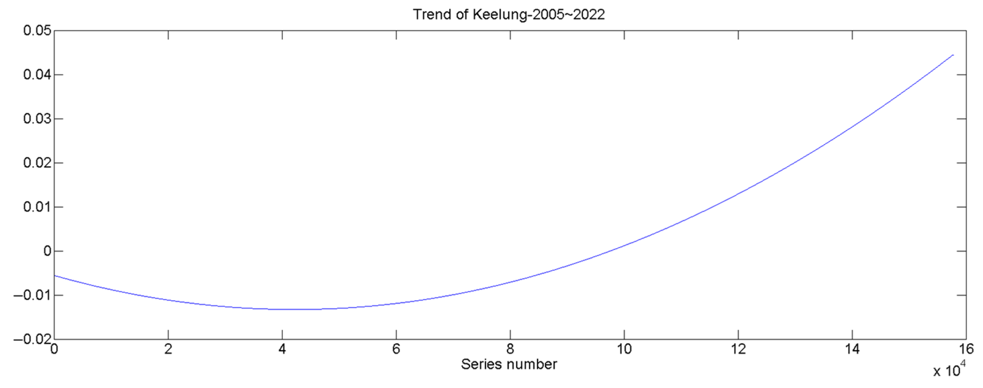
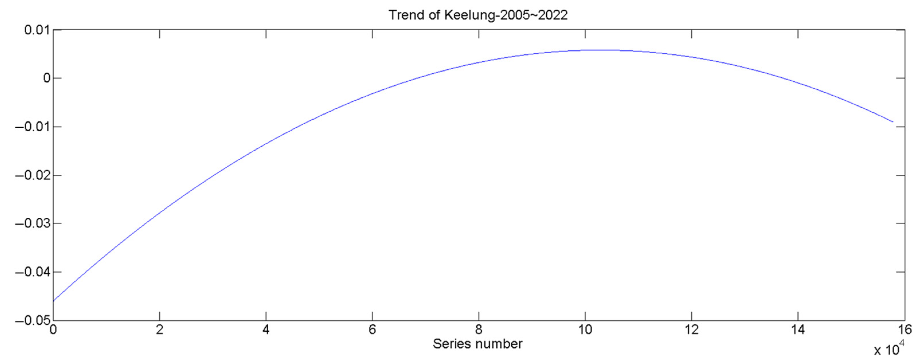
In this study, the characteristics of water level data were analyzed using the EMD method developed in [31,33]. After applying EMD to analyze the water level data from 2005 to 2022, the water level variation trend is shown in Figure 6. The estimated rise in sea level is approximately 51.20 mm, with an average sea-level-rise rate of 2.84 mm/yr. The EEMD method developed in [32] was also employed to analyze water level data. The standard deviation of the original data was 0.3, and the amplitude of the white noise was set to 0.06. The water level variation trend obtained from this analysis is illustrated in Figure 7. The estimated rise in sea level is approximately 57.73 mm, with an average sea-level-rise rate of 3.21 mm/yr. It is observed that the water level shows an initial rise followed by a decline. This trend may be attributed to the deviation caused by the end-point effect resulting from missing data. Therefore, it is not possible to infer a continued decline in the water level trend at the Keelung tide gauge station. The results of analyzing the sea level rise using the SMA, EMD, and EEMD methods for 2005 to 2022 at the Keelung tide gauge station are summarized in Table 1. The analysis results indicate that the Keelung tide gauge station’s average sea-level-rise rate ranges from 0.98 to 3.21 mm/yr.
According to the IPCC AR6 report, the global average sea-level-rise rate from 2006 to 2018 was 3.7 mm/yr. Based on the analysis of other researchers’ studies [34,35,36,37,38] in Taiwan, from 1975 to 2012, the average sea-level-rise rate ranged from 2 to 7 mm/yr. Comparing the global average sea-level-rise rate from the research report with the analyzed average sea-level-rise rate at the Keelung tide station can help assess the trend of sea level rise in the port of Keelung with the global trend, thereby increasing the credibility and significance of the study. After obtaining the sea-level-rise results, numerical models considering wave–current interactions were used, along with field observations as background data for model validation. This was performed to investigate the distribution characteristics of hydrodynamic environments near the port of Keelung under different sea-level-rise scenarios.

3. Hydrodynamic Characteristic Analysis

3.1. Model Setup

The present study aims to understand the impact of hydrodynamic characteristics on ship navigation in Keelung Harbor under different sea-level-rise scenarios. A hydrodynamic model that incorporates wave and tidal current characteristics is used for the calculations. The numerical model first analyzes the overall coastal dynamics and adjusts specific numerical parameters and input/output data formats and content for areas that may be affected. Subsequently, the model analyzes the influence of sea level rise on the wave and flow fields [39,40,41]. The calculation of the planar wave field in the hydrodynamic model utilizes the unsteady-type governing equations for water waves, including the effects of currents on inclined slopes [42]:
D 2 φ D t 2 + U D φ D t C C g φ + σ 2 k 2 C C g φ = 0
Under the assumption of non-rotational, single-frequency linear surface waves, the wave potential function can be expressed as follows:
φ x , y , z , t = f a , h φ x , y , t
where f z , h = cosh k h + z cosh k h . For the harmonic motion of waves on a single periodic wave, Equation (15) can be rewritten as follows:
φ x , y , t = Re a e i s e i ω t
The potential wave function in the equation only represents the forward-scattered wave component. It neglects the contribution from the reflected wave, which means it is not applicable when there is a significant reflection effect on the structure. By substituting Equation (16) with Equation (14) and considering the real and imaginary parts separately, the following expressions can be obtained:
Real part:
1 a C C g U a U + U 1 a 2 a + 1 C C g C C g a k 2 + s 2 = 0
Imaginary part:
a 2 σ U + C g = 0
Equations (17) and (18) represent the motion equations interacting with breaking waves and currents. When the flow velocity U is known, these two simultaneous equations can be solved to obtain the amplitude function a x , y and the wave number s . When U = 0 , Equations (17) and (18) become:
Real part:
1 a 2 a x 2 + 2 a y 2 + 1 C C g a C C g + k 2 s = 0
Imaginary part:
a 2 C C g s = 0
Furthermore, within the surf zone, energy dissipation occurs, and therefore, Equation (18) for the energy representation needs to be modified. Based on the principle of energy flux, the bed friction effects are neglected in this case:
d E C g d x = ε , ε = 1 2 ρ V e k H B 2 , V e = V e B H B / 2 c h B γ h B m , V e B = 5 S B g 8 k B ρ 1 1 C 0 , S B = tan β 1 + 3 r 2 / 2
where c represents the wave number-to-water depth ratio in the recovery zone; it is suggested that c should be set to 0.17 when the wave recovery zone is not significant in a sloping beach condition [43]. In the coexistence of wave and current interaction zone, the energy dissipation caused by nearshore currents within the surf zone is negligible and can be ignored. Therefore, according to Equation (21) for energy amplitude representation, it can be expressed as follows:
E σ U + C g = 5 16 ρ g 2 k B σ 2 tan β 1 + 3 r 2 / 2 1 1 C 0 H B / 2 c h B r h B H B 2
Using Equation (19), the energy representation within the surf zone is modified as follows, in Equation (22):
a 2 σ U + C g = 2 g ρ E σ U + C g = 5 8 g 2 k B σ 2 tan β 1 + 3 r 2 / 2 1 1 c / r H B / 2 c h B r h B H B 2
In Equations (21)–(23), the subscript “ B ” indicates the values within the surf zone. Additionally, since the phase function of ϕ is given as x x , t = s x ω t , the wave number obtained from the modified shallow water wave equation can be expressed as follows:
k = x = s
To determine the wave number s from Equations (17), (18), or (23), the knowledge of the wave direction angle is required. In other words, with only two equations involving a , s , and θ , there needs to be more information. However, assuming non-rotational gradients of the wave phase function based on linear wave theory, we can obtain the following expression:
× s = 0 s = s cos θ i + s sin θ j x s sin θ y s cos θ = 0
The tidal effect on the nearshore flow field is incorporated into the computational model in this study. Additionally, the tides are treated as long waves, considering the Coriolis effect due to the Earth’s rotation. The governing equations for the flow field, including the continuity equation and the momentum equation, can be expressed as follows:
Continuity equation:
η t + x U h + η + y V h + η = 0
Momentum equation:
U t + U U x + V U y = f V g η x + 1 ρ τ x x x + τ y x y + 1 ρ h + η τ s x τ b x 1 ρ h + η S x x x + S y x y
V t + U V x + V V y = f V g η y + 1 ρ τ x y x + τ y y y + 1 ρ h + η τ s y τ b y 1 ρ h + η S x y x + S y y y
The variables U and V represent the depth-averaged velocity components along the fixed coordinate axes x and y , respectively. Specifically:
U = 1 h + η h η u d z , V = 1 h + η h η v d z
The shear stress component τ x x , τ x y , τ y x , and τ y y includes the viscous stress caused by fluid viscosity and the Reynolds stress generated by turbulent flow effects. Comparatively, the value of viscous stress is minimal compared to Reynolds stress. Therefore, viscous stress is generally neglected, and only the Reynolds stress represents the momentum exchange between fluid particles.
τ x x = ρ E v U x , τ x y = ρ E v U y , τ y x = ρ E v V x , τ y y = ρ E v V y
where the vortex viscosity coefficient is obtained from the semi-empirical formula of Prandtl’s mixing length theory [44].
E v = k v g d + h U 2 + V 2 6 C c
The components of the wind shear stress on the sea surface represent the shear stress in the x and y directions, respectively [45].
τ s x = ρ k w W 2 cos a , τ s y = ρ k w W 2 sin a
k w = 1.2 × 10 5 , W W c 1.2 × 10 6 + 2.25 × 10 1 1 W c W 2 , W > W c
The components τ b x and τ b y of the bottom friction force represent the frictional shear stress in the x and y directions, respectively [46].
τ b x = ρ E r U U 2 + V 2 , τ b y = ρ E r V U 2 + V 2
The bottom friction coefficient is denoted as F r = g / C c 2 . The radiative stress components S x x , S x y , S y x , and S y y are the main factors causing longshore currents, represented by the linear wave theory, as follows [47]:
S x x S x y S y x S y y = E ¯ n 1 + cos 2 θ 1 2 n 2 sin 2 θ n 2 sin 2 θ n 1 + sin 2 θ 1 2
where E ¯ represents the total wave energy per unit time per unit area, in the theory of small-amplitude water waves, which can be expressed as:
E ¯ = ρ g H 2 8
The boundary conditions for the flow field are shown in Figure 8, and the water level variation includes the elevation changes caused by waves and tides.
The tidal variation is represented by a sinusoidal function, with a time lag ( T L ) indicating the time difference for the tide to reach the left and right boundaries. T s t a r t represents the phase difference:
Left boundary:
η L = A L t sin 2 π T t t + T t + T s t a r t , T t = L y g h max
Right boundary:
η R = A R t sin 2 π T t + T s t a r t
Offshore boundary:
η 0 = A R t + A L t A R t N y j N y 1 sin 2 π T t t + T t N y j N y 1 + T s t a r t
The water level induced by a wave ( ξ ¯ ) neglects the reflection effect [48]. Equation (40) represents the water level drop outside the surf zone, while Equation (41) represents the water level rise inside the surf zone:
ξ d ¯ = H 2 8 k sinh 2 k h cos θ 2 / 3
d ξ u ¯ d x = K d h d x , K = 1 1 + 8 / 3 γ 2
The left boundary of the flow velocity is given by Equation (42), the right boundary is given by Equation (43), the offshore boundary is given by Equation (44), and the alongshore boundary is given by Equation (45):
U j = 1 = U j = 2 , V y j = 1 = 0
U j = N Y = U j = N Y 1 , V y j = N Y = 0
U j = N X = U j = N X 1 , U x j = N X = 0
U = 0 , V = 0
The stability condition for the flow field calculation requires Δ t 2 Δ s g h max , where Δ s is the grid size. The maximum value of the two consecutive time steps must be smaller than the allowable error with Equation (46), and then proceed to the next time step of the calculation:
M a x η i j k + 1 η i j k ε η η i j k , ε η = 0.0001 M a x U i j k + 1 U i j k ε U U i j k , ε U = 0.0001 M a x V i j k + 1 V i j k ε V V i j k , ε V = 0.0001

3.2. Model Calculation Range and Settings

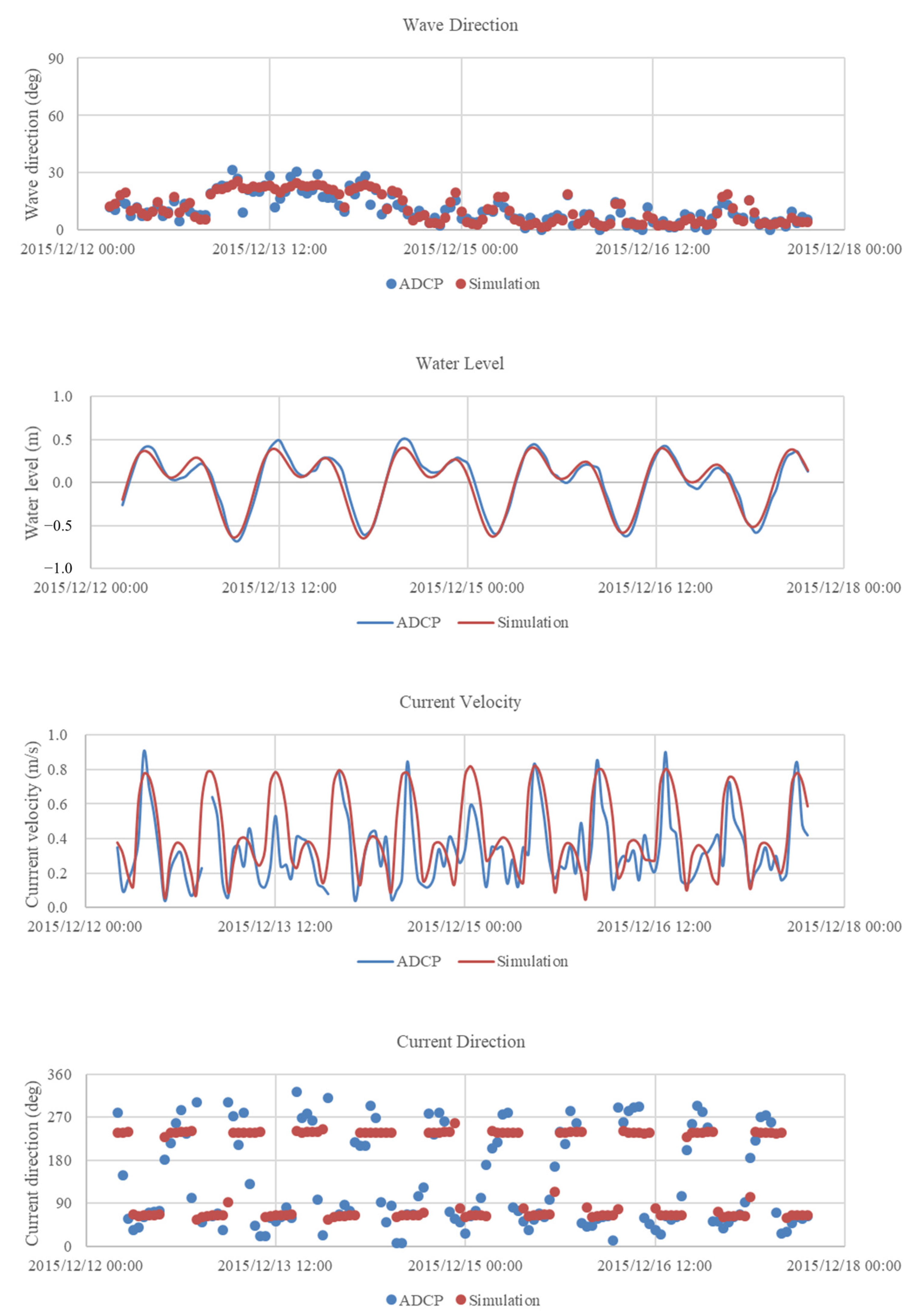
The model calculation area in this study is shown in Figure 9. It is centered around Keelung Harbor and covers a coastal distance of 5 km in the alongshore direction and 6 km in the offshore direction. The numerical topography was established using interpolated bathymetric data with a grid resolution of 200 m obtained from the National Science and Technology Council—Taiwan. The overall computational conditions of the numerical model mainly refer to the statistical data obtained from on-site observations conducted by the acoustic doppler current profiler (ADCP) installed at the port of Keelung by the Institute of Transportation, MOTC, Harbor and Marine Technology Center, as shown in Figure 1. The model settings and conditions are summarized in Table 2. The selection of the model calculation time considers the need to effectively reflect the characteristics of water flow distribution near Keelung Harbor. Therefore, the calculation is performed during the spring tide period, with a simulation period starting from minor wave conditions and gradually increasing. The comparison of model calculation results with field data is shown in Figure 10. The figure demonstrates that the water level, flow velocity, flow direction, wave height, and wave direction obtained from the model calculations generally match the field data, indicating that the model can reasonably represent the hydrodynamic characteristics in the vicinity of Keelung Harbor. Subsequently, flow field simulations were conducted for Keelung Harbor under different sea-level-rise scenarios using the validated boundary conditions and parameters. The effects of sea level rise on the regional flow field were analyzed, particularly concerning ship navigation safety.

3.3. Hydraulic Simulation Results Analysis

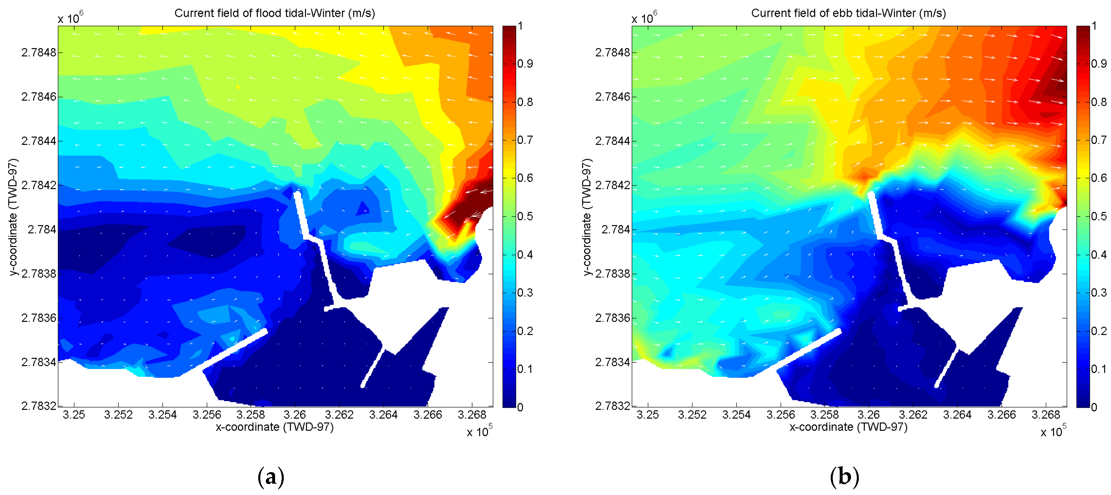
The simulated results of the model, as verified in the previous section, are presented in Figure 11. The flow characteristics in the nearshore area primarily reflect the interaction between tidal motion and the features of the nearshore topography. In the vicinity of Keelung Port, the ebb flow generally moves from west to east, while the flood flow moves from east to west. It is observed that there is an increase in flow velocity between Keelung Island and Keelung Port due to the influence of the topography. Along the outer channel to the vicinity of the revetment, during the flood tide, the average flow velocity ranges from 0.3925 to 0.6945 m/s. After entering the breakwater, the average flow velocity ranges from 0.1209 to 0.2400 m/s. The distribution of flow directions indicates the formation of a nearshore circulation pattern due to the influence of the eastern breakwater head. During the ebb tide, the average flow velocity from the outer channel to the revetment ranges from 0.6094 to 0.6906 m/s. After entering the breakwater, the average flow velocity ranges from 0.1421 to 0.4722 m/s. The flow direction is influenced by the structures, transitioning from south to north in the channel before bypassing the breakwater and then flowing eastward.
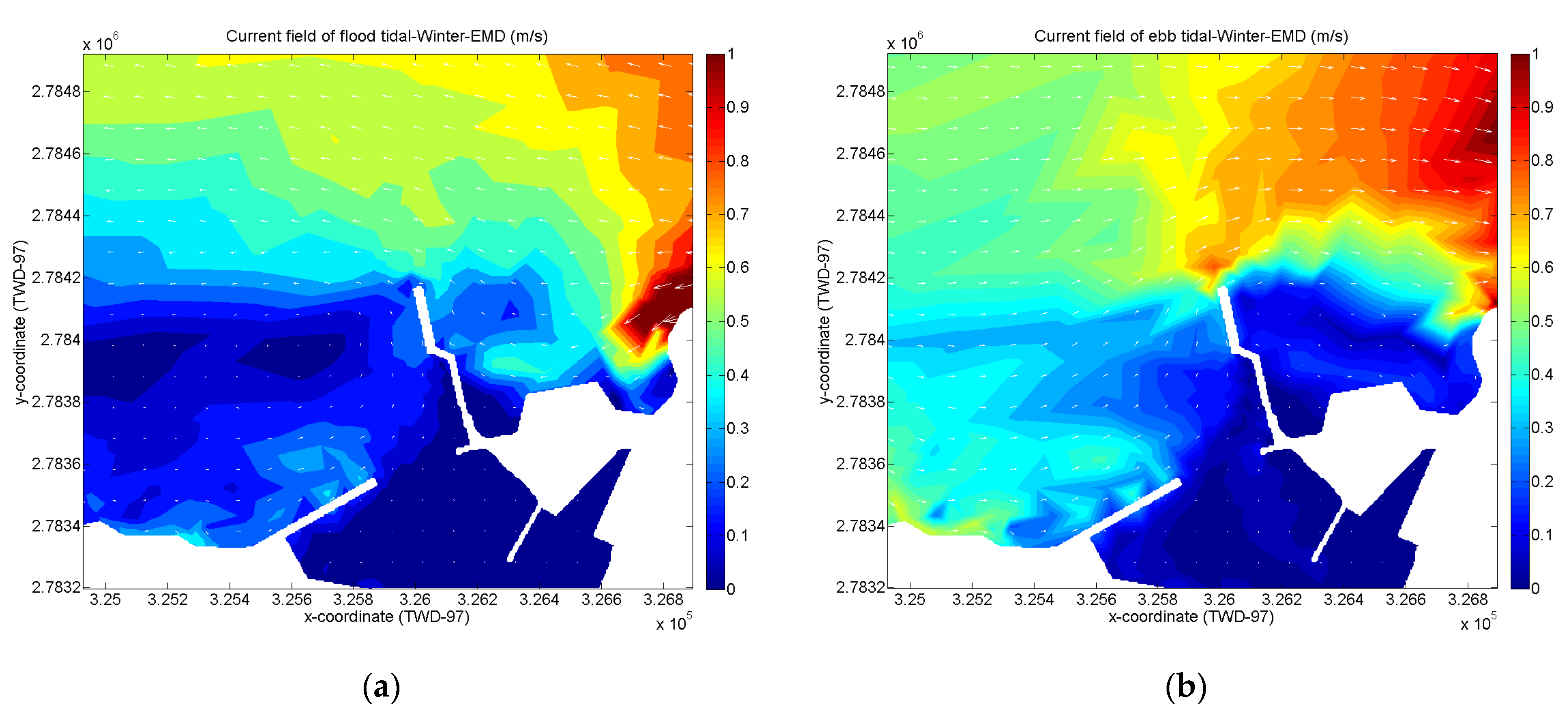
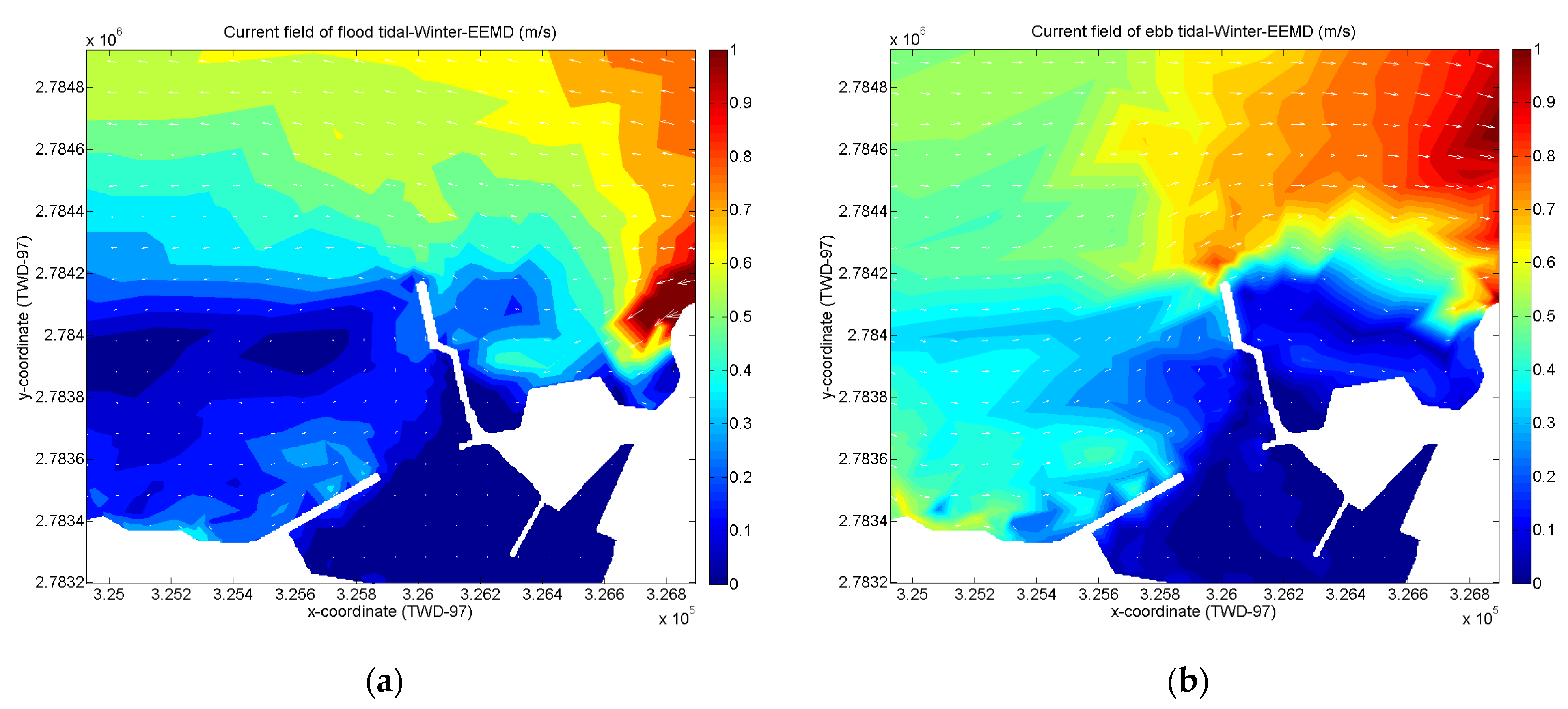
Due to the influence of environmental factors such as wind and currents, the waters from the outer channel to the vicinity of the revetment are primarily affected. Ship maneuvering is a complex process involving human, vessel, and environmental factors. The ship’s operators must process and comprehend much information to maintain or alter the vessel’s motion to achieve the intended maneuvering objectives. Various ships may face threats to their navigation in the channels due to external forces such as crosswinds and currents, which can prevent them from staying in the center of the channel. The selection of basic flow parameters is crucial for safe ship navigation. Suppose the regional water flow direction differs from the vessel’s heading. In that case, it may create a transverse flow that alters the hydrodynamic forces, pushing the ship off its intended course and compromising its safety. Large vessels are particularly susceptible to external forces during inbound and outbound sailing, making maneuvering more challenging than other vessels. Therefore, it is necessary to consider a combination of environmental forces and harbor characteristics to ensure safety. The hydraulic simulation results are obtained using different analysis methods, as shown in Figure 12, Figure 13 and Figure 14, to analyze the effects of sea level rise. For better readability, reference is made to the existing harbor channel planning in Keelung Port. The simulated results are extracted near the “main fairway sector” indicated in Figure 1, and data extraction and discussion are conducted along the inbound fairway at 150 m intervals.
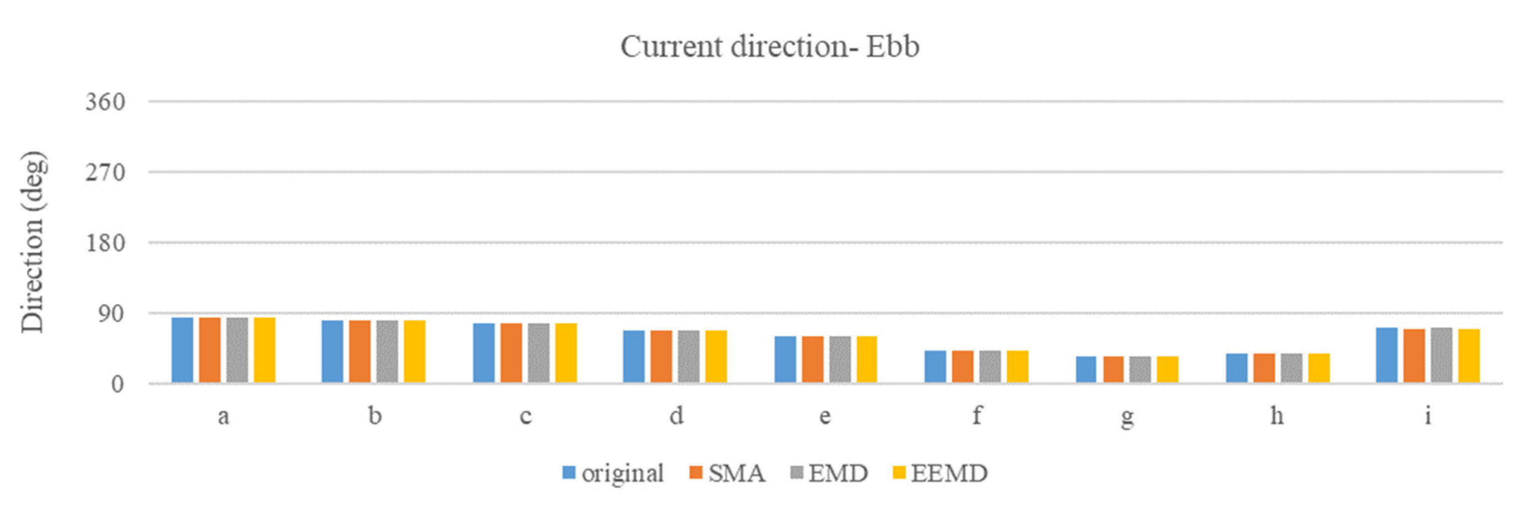
The simulation results, shown in Figure 15 and Figure 16 and summarized in Table 3 and Table 4, provide a visual representation and quantification of the current pattern along the inbound and outbound fairways at 150 m intervals. In the vicinity of the outer fairway to the entrance (a–e), the simulated results under different sea-level-rise conditions provide valuable insights when incorporating different methods such as SMA, EMD, and EEMD. During the rise tide, the average current velocity ranges from 0.3926 to 0.6945 m/s when utilizing the SMA method, from 0.3926 to 0.6946 m/s with the EMD method, and from 0.3927 to 0.6947 m/s with the EEMD method. On the ebb tide, the average current velocity ranges from 0.6129 to 0.6866 m/s (SMA), 0.6135 to 0.6871 m/s (EMD), and 0.6166 to 0.6901 m/s (EEMD). After entering the entrance (f–e), the current velocity generally decreases as it enters the harbor area. During the flood tide, the average current velocity ranges from 0.1210 to 0.2401 m/s (SMA), 0.1210 to 0.2402 m/s (EMD), and 0.1211 to 0.2402 m/s (EEMD). On the ebb tide, the average current velocity ranges from 0.1429 to 0.4752 m/s (SMA), 0.1435 to 0.4757 m/s (EMD), and 0.1440 to 0.4783 m/s (EEMD). It is observed that the current velocity generally increases from the outer fairway to inside the entrance (a–i) as sea levels rise, indicating the influence of hydrodynamics and the impact of changing water levels on current patterns. Conversely, the distribution of flow direction shows less significant changes, suggesting that the dominant direction of current remains relatively consistent despite variations in sea level.
The results of the simulations provide a basis for discussion and a theoretical analysis of the flow velocity patterns under different sea-level-rise conditions in the studied area, particularly in the vicinity of the outer fairway to the entrance (a–e). By utilizing the simulation results, potential hazards and issues can be identified, aiding mariners in conducting safety assessments and devising effective navigational strategies based on the actual distribution of current. Overall, this comprehensive analysis of the simulation results provides valuable insights into the current characteristics within the studied area, aiding in understanding the impact of sea level rise and enhancing navigational safety considerations.

4. Conclusions

In the past, sea level rise has been assessed using linear regression and the least squares method to determine coefficients. Additionally, traditional harmonic analysis methods have been unable to analyze sea level rise. Therefore, this study examines the impact of sea level rise on ship navigation safety by analyzing changes in current characteristics. Three analysis methods, SMA, EMD, and EEMD, were employed to investigate sea-level-rise trends from 2005 to 2022 at the Keelung tide gauge station. The SMA analysis indicated an average sea level rise of 0.98 mm/yr, totaling approximately 17.68 mm. The EMD analysis showed an average rise of 2.84 mm/yr, reaching around 51.20 mm. The EEMD analysis revealed the highest average rise of 3.21 mm/yr, approximately 57.73 mm. However, the EEMD analysis also indicated a declining trend, possibly influenced by data gaps and endpoint effects. It was challenging to ascertain a continuous downward trend in water levels at the Keelung tide gauge station.
Due to the external forces acting on a vessel, including wind (on the water surface), currents (underwater), and waves (affecting vessel stability), understanding the magnitude and direction of current is crucial for effective vessel maneuvering. When a vessel carries cargo, its draft increases, increasing the current impact area. The velocity and direction of the currents are influenced by harbor structures, leading to variations. Moreover, the current pressure exerted on the vessel by the current changes with the vessel’s heading angle during navigation. Therefore, understanding the magnitude and direction of current is significantly beneficial for subsequent vessel operations. Therefore, using the obtained sea-level-rise data, hydrodynamic simulations were conducted, focusing on the outer fairway to the entrance area. During the flood tide, current velocities ranged from 0.3926 to 0.6945 m/s (SMA), 0.3926 to 0.6946 m/s (EMD), and 0.3927 to 0.6947 m/s (EEMD). On the ebb tide, current velocities in the same area ranged from 0.6129 to 0.6866 m/s (SMA), 0.6135 to 0.6871 m/s (EMD), and 0.6166 to 0.6901 m/s (EEMD). Upon entering the harbor area, current velocities generally decreased. During the flood tide, velocities ranged from 0.1210 to 0.2401 m/s (SMA), 0.1210 to 0.2402 m/s (EMD), and 0.1211 to 0.2402 m/s (EEMD). On the ebb tide, velocities ranged from 0.1429 to 0.4752 m/s (SMA), 0.1435 to 0.4757 m/s (EMD), and 0.1440 to 0.4783 m/s (EEMD). The current velocity distribution from the outer fairway to the entrance generally increased with sea level rise, while changes in current direction distribution were less pronounced. Since selecting basic current parameters is crucial for vessel navigation, these analysis results offer valuable insights for mariners to assess navigation safety and devise appropriate strategies based on the actual flow conditions. Furthermore, they can serve as a reference for maritime and management authorities in ensuring safe navigation in harbor fairways.

Author Contributions

Conceptualization, T.-H.C. and H.-Y.W.; software, H.-Y.W.; validation, T.-H.C. and H.-Y.W.; formal analysis, T.-H.C. and H.-Y.W.; data curation, H.-Y.W.; writing—original draft preparation, H.-Y.W.; visualization, H.-Y.W.; project administration, T.-H.C. All authors have read and agreed to the published version of the manuscript.

Funding

This research received no external funding.

Data Availability Statement

Not applicable.

Conflicts of Interest

The authors declare no conflict of interest.

References

  1. Douglas, B.C. Chapter 3 Sea level change in the era of the recording tide gauge. In International Geophysics; Elsevier: Amsterdam, The Netherlands, 2001; Volume 75, pp. 37–64. [Google Scholar]
  2. Mitrovica, J.X.; Tsimplis, M.E.; Davis, J.L.; Milne, G.A. Recent mass balance of polar ice sheets inferred from patterns of global sea-level change. Nature 2001, 409, 1026–1029. [Google Scholar] [CrossRef] [PubMed]
  3. Church, J.A.; White, N.J.; Coleman, R.; Lambeck, K.; Mitrovica, J.X. Estimates of regional distribution of sea level rise over the 1950–2000 period. J. Clim. 2004, 17, 2609–2625. [Google Scholar] [CrossRef]
  4. Church, J.; White, N.J. Sea-level rise from the late 19th to the Early 21st Century. Surv. Geophys. 2011, 32, 585–602. [Google Scholar] [CrossRef] [Green Version]
  5. Shum, C.K.; Kuo, C.Y. Observation and geophysical causes of present-day sea level rise. In Climate Change and Food Security in South Asia; Springer: Dordrecht, The Netherlands, 2011; pp. 85–104. [Google Scholar]
  6. Merrifield, M.A.; Merrifield, S.T.; Mitchum, G.T. An Anomalous Recent Acceleration of Global Sea Level Rise. J. Clim. 2009, 22, 5772–5781. [Google Scholar] [CrossRef] [Green Version]
  7. Allan, R.P.; Hawkins, E.; Bellouin, N.; Collins, B. IPCC, 2021: Summary for Policymakers. In Climate Change 2021: The Physical Science Basis. Contribution of Working Group I to the Sixth Assessment Report of the Intergovernmental Panel on Climate Change; Masson-Delmotte, V., Zhai, P., Pirani, A., Connors, S.L., Péan, C., Berger, S., Caud, N., Chen, Y., Goldfarb, L., Gomis, M.I., et al., Eds.; Cambridge University Press: Cambridge, UK, 2023; in press. [Google Scholar]
  8. Rahmstorf, S. A semi-empirical approach to projecting future sea level rise. Science 2007, 315, 368–370. [Google Scholar] [CrossRef] [Green Version]
  9. Rahmstorf, S. Response to comment on “A semi-empirical approach to projecting future sea level rise”. Science 2007, 317, 1866. [Google Scholar] [CrossRef] [Green Version]
  10. Horton, R.; Herweijer, C.; Rosenzweig, C.; Liu, J.; Gornitz, V.; Ruane, A.C. Sea level rise projections for current generation CGCMs based on the semi-empirical method. Geophys. Res. Lett. 2008, 35, L02715. [Google Scholar] [CrossRef]
  11. Zhan, J.G.; Wang, Y.; Cheng, Y.S. The analysis of China sea level change. Chin. J. Geophys. 2009, 52, 1725–1733. (In Chinese) [Google Scholar]
  12. Wisha, U.J.; Wijaya, Y.J.; Hisaki, Y. Sea Level Variability in the Equatorial Malacca Strait: The Influence of Climatic–Oceanographic Factors and Its Implications for Tidal Properties in the Estuarine Zone. Climate 2023, 11, 70. [Google Scholar] [CrossRef]
  13. Iglesias, I.; Bio, A.; Melo, W.; Avilez-Valente, P.; Pinho, J.; Cruz, M.; Gomes, A.; Vieira, J.; Bastos, L.; Veloso-Gomes, F. Hydrodynamic Model Ensembles for Climate Change Projections in Estuarine Regions. Water 2022, 14, 1966. [Google Scholar] [CrossRef]
  14. Aguilera-Vidal, M.; Muñoz-Perez, J.J.; Contreras, A.; Contreras, F.; Lopez-Garcia, P.; Jigena, B. Increase in the Erosion Rate Due to the Impact of Climate Change on Sea Level Rise: Victoria Beach, a Case Study. J. Mar. Sci. Eng. 2022, 10, 1912. [Google Scholar] [CrossRef]
  15. KobaYashi, H.; Endo, M. The Ship Maneuverability Effect on the Safety Assessment of Navigation. Jpn. Inst. Navig. 1994, 120, 8–14. (In Japanese) [Google Scholar]
  16. Arai, Y.; Fukuto, J. Natural environmental conditions in safety evaluation of navigation environment. Jpn. Inst. Navig. 1994, 120, 15–20. (In Japanese) [Google Scholar]
  17. Goossens, L.H.J.; Glansdorp, C.C. Operational benefits and risk reduction of marine accidents. J. Navig. 1998, 51, 369–381. [Google Scholar] [CrossRef]
  18. Gucma, L. Navigation risk assessment for vessels manoeuvring in various conditions. WIT Trans. Model. Simul. 2002, 31, 149–158. [Google Scholar]
  19. Akten, N. Analysis of shipping casualties in the Bosporus. J. Navig. 2004, 57, 345–356. [Google Scholar] [CrossRef]
  20. Gucma, L. The risk assessment of ships manoeuvring on the waterways based on generalized simulation data. WIT Trans. Built Environ. 2007, 94, 411–418. [Google Scholar]
  21. Yip, T.L. Port traffic risks—A study of accidents in Hong Kong waters. Transp. Res. Part E Logist. Transp. Rev. 2008, 44, 921–931. [Google Scholar] [CrossRef]
  22. Szelangiewicz, T.; Wiśniewski, B.; Żelazny, K. The influence of wind, wave and loading condition on total resistance and speed of the vessel. Pol. Marit. Res. 2014, 21, 61–67. [Google Scholar] [CrossRef] [Green Version]
  23. Chen, C.; Shiotani, S.; Sasa, K. Effect of ocean currents on ship navigation in the East China Sea. Ocean. Eng. 2015, 104, 283–293. [Google Scholar] [CrossRef]
  24. Toffoli, A.; Lefèvre, J.M.; Bitner-Gregersen, E.; Monbaliu, J. Towards the identification of warning criteria: Analysis of a ship accident database. Appl. Ocean. Res. 2005, 27, 281–291. [Google Scholar] [CrossRef]
  25. Rusu, E. Modelling of wave-current interactions at the mouths of the Danube. J. Mar. Sci. Technol. 2010, 15, 143–159. [Google Scholar] [CrossRef]
  26. Arslan, O.; Turan, O. Analytical investigation of marine casualties at the Strait of Istanbul with SWOT-AHP method. Marit. Policy Manag. 2011, 36, 131–145. [Google Scholar] [CrossRef] [Green Version]
  27. Chen, C. Case Study on Wave-Current Interaction and its Effects on Ship Navigation. J. Hydrodyn. 2018, 30, 411–419. [Google Scholar] [CrossRef]
  28. Lee, C.C. Safety Manoeuvring Tendency for Ship in/out-port of Taichung. J. Taiwan Marit. Saf. Secur. Stud. 2013, 4, 1–18. (In Chinese) [Google Scholar]
  29. Chou, C.C.; Chen, C.Y.; Chang, P.C.; Chang, T.M.; Hsu, H.Z.; Chang, K.E. Use the grid to analyze the influential factors on marine accidents. Lect. Notes Electr. Eng. 2014, 293, 867–874. [Google Scholar]
  30. Chou, C.C.; Su, Y.L.; Li, R.F.; Tsai, C.L.; Ding, J.F. Key navigation safety factors in Taiwanese harbours and surrounding waters. J. Mar. Sci. Technol. 2015, 23, 685–693. [Google Scholar]
  31. Huang, N.E.; Shen, Z.; Long, S.R.; Wu, M.L.; Shih, H.H.; Zheng, Q.; Yen, N.C.; Tung, C.C.; Liu, H.H. The empirical mode decomposition and Hilbert spectrum for nonlinear and non-stationary time series analysis. Proc. R. Soc. Lond. A 1998, 454, 903–995. [Google Scholar] [CrossRef]
  32. Wu, Z.; Huang, N.E. Ensemble empirical mode decomposition: A noise-assisted data analysis method. Adv. Adapt. Data Anal. 2009, 1, 1–41. [Google Scholar] [CrossRef]
  33. Huang, N.E.; Shen, Z.; Long, S.R. A new view of nonlinear water waves: The Hilbert spectrum. Annu. Rev. Fluid Mech. 1999, 31, 417–457. [Google Scholar] [CrossRef] [Green Version]
  34. Chen, Y.W. A Study on the Relationship between Climatic Factors and Sea Level Height Fluctuation of Keelung and Kaohsiung Ports. Master’s Thesis, National Taiwan Ocean University, Keelung, Taiwan, 2003. (In Chinese). [Google Scholar]
  35. Doong, D.J.; Tzeng, K.T.; Yang, I.S. Sea Level Fluctuation at Keelung and Kaohsiung. In Proceedings of the 30th Ocean Engineering Conference in Taiwan, Hsinchu, Taiwan, 13–14 November 2008; pp. 625–630. (In Chinese). [Google Scholar]
  36. Sung, Y.P. Prediction of Sea-Level Change around Taiwan by Using Tides and Satellite Data. Master’s Thesis, National Cheng Kung University, Tainan, Taiwan, 2012. (In Chinese). [Google Scholar]
  37. Lan, W.H. Assessment of Seasonal-to-Decadal Variability and Trends of Regional Sea Level in the North Pacific Ocean Using Satellite Altimetry and Tide Gauges. Ph.D. Thesis, National Cheng Kung University, Tainan, Taiwan, 2018. (In Chinese). [Google Scholar]
  38. Lan, W.H.; Kuo, C.Y.; Lin, S.F. Impact of sea level variations on hydrographic survey. Taiwan J. Geoinformatics 2022, 10, 99–120. (In Chinese) [Google Scholar]
  39. Chiang, Y.C.; Hsiao, S.S.; Lin, M.C. A Quasi-3D Sediment Transport Modeling for Coastal Morphodynamics. In Proceedings of the 21st International Offshore and Polar Engineering Conference, Maui, HI, USA, 19–24 June 2011; pp. 1053–1058. (In Chinese). [Google Scholar]
  40. Chiang, Y.C.; Hsiao, S.S. Coastal Morphological Modeling. In Sediment Transport in Aquatic Environments; InTech: Rijeka, Croatia, 2011; Chapter 10; pp. 203–230. [Google Scholar]
  41. Wang, H.Y.; Fang, H.M.; Hsiao, S.S. Morphological Characteristics of Tidal Inlets Subject to a Short Term Typhoon Event: A Case Study in Lanyan River Estuary. J. Mar. Sci. Technol. 2018, 26, 552–561. [Google Scholar]
  42. Kirby, J.T. A parabolic equation for the combined refraction-diffraction of Stokes waves by mildly varying topography. J. Fluid Mech. 1983, 136, 453–466. [Google Scholar] [CrossRef] [Green Version]
  43. Mizuguchi, M. An heuristic model of wave height distribution in surf zone. In Coastal Engineering 1980; American Society of Civil Engineers: Reston, VA, USA, 1980; pp. 278–289. [Google Scholar]
  44. Falconer, R.A. Numerical modeling of tidal circulation in harbors. J. Waterw. Port Coast. Ocean. Div. 1980, 106, 31–48. [Google Scholar] [CrossRef]
  45. Dean, R.G.; Dalrymple, R.A. Water Wave Mechanics for Engineers and Scientists; World Scientific Publishing Company: Singapore, 1984; Volume 2. [Google Scholar]
  46. Ponce, V.M.; Yabusaki, S.B. Modeling circulation in depth-averaged flow. J. Hydraul. Div. 1981, 107, 1501–1518. [Google Scholar] [CrossRef]
  47. Longuet-Higgins, M.S.; Stewart, R.W. Radiation stresses in water waves; a physical discussion, with applications. Deep. Sea Res. Oceanogr. Abstr. 1964, 11, 529–562. [Google Scholar] [CrossRef]
  48. Matushevskiy, T.V. Method of separation of wave induced and turbulent motions in the near-surface layer of the ocean. In On Problems of Ocean Dynamics; Gidrometeoizdat: Leningrad, Russia, 1975; pp. 124–151. (In Russian) [Google Scholar]
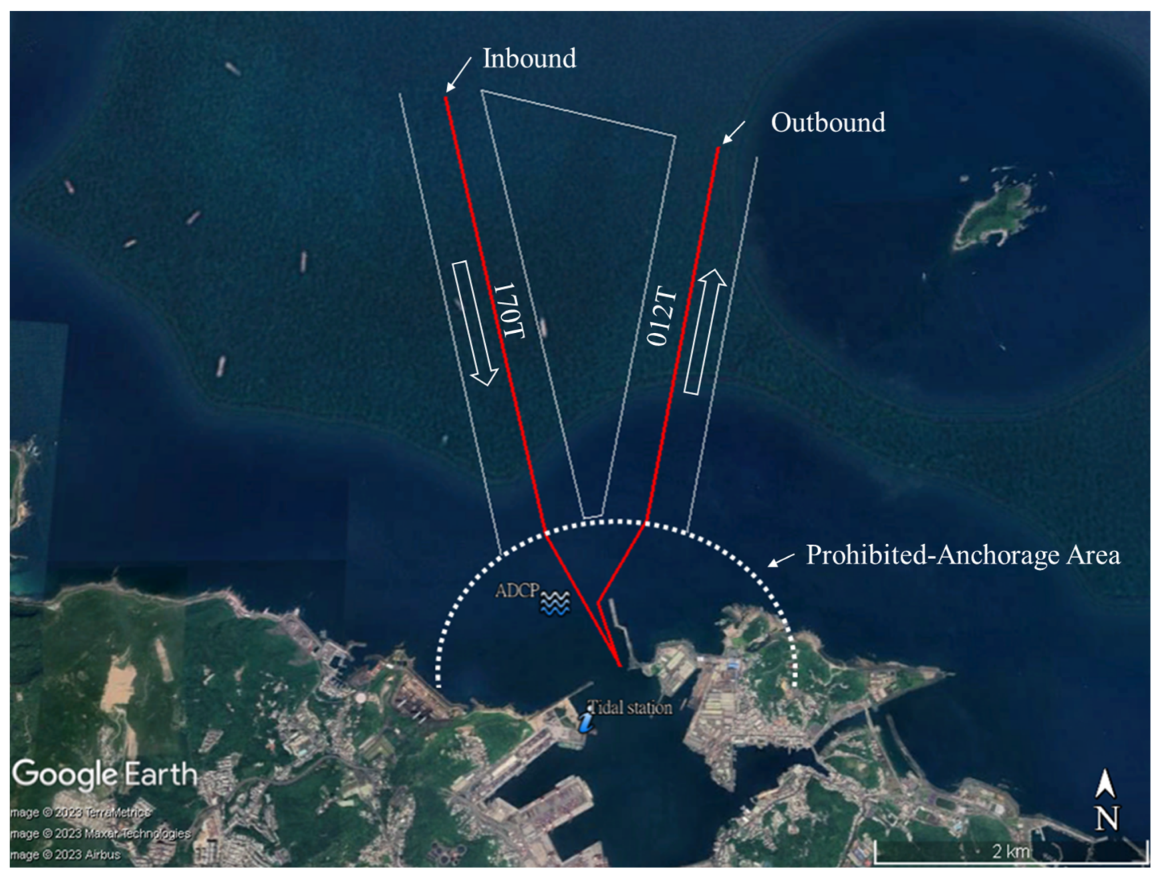
Figure 1. Location of the Keelung Port water level, wave, and current measurement stations.
Water 15 02570 g001
Figure 2. Time series of the original water level data.
Water 15 02570 g002
Figure 3. Time series plot of the supplemented water level data after harmonic analysis.
Water 15 02570 g003
Figure 4. Analysis of average sea level rise using SMA.
Water 15 02570 g004
Figure 5. Schematic diagram of the HHT analysis process.
Water 15 02570 g005
Figure 6. Analysis of average sea level rise using EMD.
Water 15 02570 g006
Figure 7. Analysis of average sea level rise using EEMD.
Water 15 02570 g007
Figure 8. Boundary conditions in the flow field.
Water 15 02570 g008
Figure 9. Model setup area.
Water 15 02570 g009
Figure 10. Comparison between the numerical model and the measured data. Blue line: Measurement data. Red line: Simulation results.
Water 15 02570 g010aWater 15 02570 g010b
Figure 11. Simulation results of the flow field under original conditions. (a) Flood tide. (b) Ebb tide.
Water 15 02570 g011
Figure 12. Simulation results of the flow field under SMA conditions. (a) Flood tide. (b) Ebb tide.
Water 15 02570 g012
Figure 13. Simulation results of the flow field under EMD conditions. (a) Flood tide. (b) Ebb tide.
Water 15 02570 g013
Figure 14. Simulation results of the flow field under EEMD conditions. (a) Flood tide. (b) Ebb tide.
Water 15 02570 g014
Figure 15. Flow velocity and direction distribution within the outer fairway to the breakwater (a–i) under flood tide conditions.
Water 15 02570 g015
Figure 16. Flow velocity and direction distribution within the outer fairway to the breakwater (a–i) under ebb tide conditions.
Water 15 02570 g016aWater 15 02570 g016b
Table 1. Analysis results of sea level rise.
Analysis MethodAvg. SLRAvg. SLR Rate
SMA17.68 mm0.98 mm/yr
EMD51.20 mm2.84 mm/yr
EEMD57.73 mm3.21 mm/yr
Table 2. Simulation conditions.
ItemModel Setup
Area5 km × 6 km
Grid size Δ x = Δ y = 25 m
Number of grid points200 × 240
Time step Δ t = 2 s
Time scale1.0
Wave condition2.5 m; 8.0 s; NNE
Table 3. Statistics table of flow velocity and direction within the outer fairway to the breakwater (a–i) under flood tide conditions.
OriginalSMAEMDEEMD
V (m/s)Dir.V (m/s)Dir.V (m/s)Dir.V (m/s)Dir.
a0.6943272.720.6945272.720.6946272.730.6947272.73
b0.6706271.070.6707271.080.6709271.080.6709271.08
c0.6033269.170.6034269.180.6035269.200.6036269.20
d0.4952268.050.4953268.080.4953268.130.4954268.13
e0.3925266.770.3926266.820.3926266.900.3927266.90
f0.2400293.970.2401294.030.2402294.120.2402294.11
g0.1623351.560.1624351.590.1626351.630.1626351.62
h0.197527.900.197627.870.197727.800.197727.80
i0.120931.430.121031.330.121031.120.121131.13
Table 4. Statistics table of flow velocity and direction within the outer fairway to the breakwater (a–i) under ebb tide conditions.
OriginalSMAEMDEEMD
V (m/s)Dir.V (m/s)Dir.V (m/s)Dir.V (m/s)Dir.
a0.683484.040.686683.980.687183.970.690183.91
b0.690680.700.694080.650.694580.640.697780.58
c0.671475.960.674975.900.675475.890.678675.84
d0.637067.680.640567.630.641067.620.644167.57
e0.609459.680.612959.640.613559.630.616659.59
f0.472242.570.475242.540.475742.530.478342.51
g0.353133.850.355533.830.356133.830.358033.80
h0.261438.180.263438.110.263838.150.265438.07
i0.142170.360.142970.210.143570.250.144070.11
Disclaimer/Publisher’s Note: The statements, opinions and data contained in all publications are solely those of the individual author(s) and contributor(s) and not of MDPI and/or the editor(s). MDPI and/or the editor(s) disclaim responsibility for any injury to people or property resulting from any ideas, methods, instructions or products referred to in the content.