Tidal Currents in Douglas Channel, British Columbia: Evaluation and Prediction

Abstract

Douglas Channel is the principal shipping route between the town of Kitimat and the Pacific Ocean. Prediction of near-surface currents is crucial for safe tanker navigation and cleaning-up oil spills. Three years of current velocity data were collected at two moorings located 30 km apart. Spectral, wavelet, and harmonic analysis of measured currents throughout the upper (40-m) and lower (50–358 m) water columns indicated the predominant influence of semidiurnal (SD) tidal currents. In the upper layer, wind and density flows resulted in considerable seasonal and interannual variability of these currents. Analysis of the SD variance reveals three major components: barotropic, coherent baroclinic, and random baroclinic. The predictability of near-surface currents depends on the relative contribution and stability of the first two components. Tidal constants estimated for one year were used to predict currents for two other years; we found that at the mooring closer to the entrance of Douglas Channel, 80 to 89% of the SD energy in the upper layer and 89–93% in the lower layer can be forecasted, while closer to the two channel head, these numbers are smaller: 55–70% and 79–89%, respectively.

1. Introduction

Douglas Channel is one of the most important inlets on the British Columbia coast. Its length from the head of Kitimat Arm to Wright Sound, on the Inside Passage ferry route, is about 90 km. The overall length of the fjord‘s waterway extending from the town of Kitimat to the open waters of Hecate Strait is 140 km. The system of multiple channels connecting Kitimat with the coastal waters of British Columbia is frequently referred to as the “Kitimat fjord system” [1,2]. The system is the principal shipping route between the town of Kitimat and the Pacific Ocean. The further plans for the development of Kitimat include several plants and liquified natural gas terminals. One of the most important elements of hydrodynamical investigation, crucial for safe navigation and cleaning up of tanker-induced oil spills, is the examination of near-surface circulation along the shipping route and adjacent passages [3]. Three principal current velocity components determining this circulation are tidal, wind-driven, and estuarine circulation [4].

In 2013 the Government of Canada launched a program to collect physical, geochemical, and biological data in the Kitimat fjord system. Observational data were collected from July 2013 to July 2016. In particular, two moorings, KSK and FOC, were deployed in Douglas Channel for 3 years (Figure 1). The data from these moorings, as well as from two tide gauges located nearby, are used to examine the dynamical parameters of the Kitimat fjord system, in particular the sea level oscillations and currents within the system.

The topic of the present study is tidal currents. Tides are strong in Douglas Channel; the tidal range is up to 6.5 m. Tides in this region are mainly semidiurnal (SD); consequently, SD tidal currents strongly prevail. Typical SD current magnitudes are 10 cm/s with intense currents in narrows exceeding several knots. Webster [4] found that the near-surface M2 tidal currents in this region exhibit substantial temporal variability, indicating the importance of a baroclinic component to the M2 tide. Therefore, the main objective is the characterization of the variability in the M2 tidal currents at the KSK and FOC moorings, evaluation of seasonal changes in these currents, and partitioning them into barotropic, coherent baroclinic, and stochastic parts. Based on the results we estimated the predictability of tidal currents in the Kitimat fjord system.

However, the M2 currents and semidiurnal currents do not exist in isolation: they are superimposed on diurnal and shallow-water tidal currents, as well as on wind-driven currents and estuarine circulation. Detailed analysis of these low-frequency currents in the Douglas Channel was recently carried out by Wan et al. [5,6]. To estimate the relative importance of the M2 currents, we compared them with other types of the observed currents.

Although the results of this paper are related to a specific region (Douglas Channel/Kitimat fjord system), we believe that they reflect some general properties of tidal, estuarine, and wind-driven currents in tidal fjords, in particular those in Alaska and Norway. From this point of view, our results and approaches could be useful for analyses of coastal currents around the world.

2. Materials and Methods

Figure 1 shows the location of moorings KSK and FOC in the study area. The moorings had various combinations of instruments: single-point current meters (Aquadopps), Acoustic Doppler Current Profilers (ADCP), and conductivity, temperature, and depth sensors (CTD). The distribution of observations in the vertical varies by year and location, however, there is always an upwards-looking ADCP at about 40 m depth. The list of the instruments for the three deployments (A, B, and C) used in the study is presented in

Table 1. List of the instruments for three deployments (2013–2014, 2014–2015, and 2015–2016) at stations KSK and FOC in Douglas Channel, British Columbia.

Deployment Time Period (dd/mm/yyyy)	A 2 July 2013–1 July 2014	B 3 July 2014–25 July 2015	C 26 July 2015–19 May 2016
	Station KSK (53.48º N; 129.209º W)
Instruments ADCP up	11 (4 m), 6–46 m, 15 min	16 (2 m), 4.7–34.7 m, 30 min	14 (2 m), 12–38 m, 30 min
ADCP down	-	20 (16 m), 35–339 m, 30 min	19 (16 m), 47–335 m, 30 min
Aquadopp-1	152 m, 60 min	154 m, 15 min	-
Aquadopp-2	322 m, 60 min	-	-
CTD	322 m, 30 min	359 m, 30 min	370 m, 30 min
	Station FOC (53.7356º N; 129.03º W)
Instruments ADCP up	14 (2 m), 10–36 m, 15 min	7 (4 m), 5.2–29.2 m, 30 min	14 (2 m), 7–33 m, 30 min
ADCP down	22 (4 m), 274–358 m, 30 min	25 (4 m), 263–359 m, 30 min	19 (16 m), 43.5–331.5 m, 30 min
Aquadopp-1	53.5 m, 60 min	51.3 m, 30 min	-
Aquadopp-2	201 m, 60 min	151.5, 30 min	-
CTD	315 m, 30 min	300 m, 10 min	322 m, 30 min

Note: Comment: For ADCP the number of bins, bin interval, upper and lower bin depths, and sampling interval are indicated; for other instruments the depth and sampling interval is given.

. Additional information about the instruments used at moorings KSK and FOC can be found in [7,8,9].

The lengths of the series in each deployment, for almost all instruments, were approximately one year; the sampling intervals ranged from 10 to 60 min (Table 1). Such series lengths and samplings enable us to precisely estimate the mean amplitudes and phases of more than 60 tidal constituents. Moreover, these data allow us to examine seasonal variations of baroclinic tides and compare them for three different years.

To examine the data, we used spectral analysis of individual velocity components U and V and bottom pressure, rotary spectral analysis (of current velocity components) [10,11,12], wavelet analysis of sea levels and currents [12], and harmonic analysis of tides by the least squares method [13,14,15]. The general procedure of the current velocity analysis is similar to that one that was used to examine current velocities in the Beaufort Sea [16]. To estimate seasonal variations of tidal currents we separated the 3-year ADCP series into individual monthly series and performed harmonic analysis of tides for each of these series.

3. Tidal Analysis of Sea Level and Currents

3.1. Sea Level Tidal Analysis

To examine sea level tidal oscillations at moorings KSK and FOC, we used bottom pressure time series from Sea-Bird CTDs deployed at these moorings. The frequency properties of sea level oscillations in the Douglas Channel were estimated based on the spectral analysis procedure similar to that described by Thomson and Emery [12]. To improve the spectral estimates, we used a Kaiser-Bessel (KB) spectral window with half-window overlaps prior to the Fourier transform. The length of the window was N = 4096 for 30-min records and N = 2048 for 60-min records (85.3 days), yielding ν = 14 degrees of freedom. As an example, the computed spectrum for Mooring KSK, Deployment A is presented in Figure 2 (spectra for other KSK deployments and Mooring FOC look very similar).

The spectrum of the background oscillations is “red”, with spectral energy gradually decreasing with increasing frequency according to the ω⁻² power law. The main property of the spectrum is strong discrete peaks at the frequencies of the major tidal constituents. The spectral peaks associated with semidiurnal tides are predominant, but diurnal peaks are also quite strong. Evident spectral peaks at frequencies of shallow-water high-frequency tidal harmonics (~3, 4, 5, and 6 cycles per lunar day) indicate an important role of nonlinear processes in the formation of the tides in this region.

To calculate the mean amplitudes and phases of tidal constituents, including long-period and shallow-water constituents, we used the least squares method [13,15]. The results of these computations enabled us to estimate initial, tidal, and residual variances of bottom pressure records, as well as the range of tidal oscillations and some other important tidal parameters. According to the results shown in

Table 2. Estimated initial, tidal, and residual variances of bottom pressure at Moorings KSK and FOC (Deployments A, B, and C). The tidal ranges for each mooring and deployment are given.

Moorings, Years	Sampling (min)	Variance				Range (m)
		Initial (cm2)	Tidal (cm2)	Residual (cm2)	Residual (%)
KSK
A 2013–2014	30	17,345	17,316	28	0.16	6.31
B 2014–2015	30	17,573	17,517	56	0.32	6.20
C 2015–2016	30	17,762	17,715	47	0.27	6.57
FOC
A 2013–2014	30	18,183	18,152	31	0.17	6.40
B 2014–2015	10	18,384	18,326	58	0.32	6.36
C 2015–2016	60	18,658	18,610	48	0.26	6.64

, approximately 99.7–99.8% of the bottom pressure variances are associated with tides. The small amount of the residual (non-tidal) variance is mainly related to the fact that the instrument measures, not real sea level oscillations, but the weight of the water column, excluding the inverted barometer sea level response to the air pressure variations or to steric sea level changes, which do not change this weight. However, these problems do not affect gravitational tidal harmonics. The total range of tides in this region is quite high, about 6.5 m (Table 2), indicating the primary importance of tidal oscillations for the dynamics of the Kitimat fjord system.

The quality of tidal prediction was quite high; the spectra of the residual series (Figure 2) do not contain any noticeable peaks at frequencies of diurnal and semidiurnal tides. While the root mean square (σ_init) of the recorded oscillations was 131–136 cm, the residual deviation (σ_res) was only 5.3–7.6 cm. The mean amplitudes and phases of 10 major tidal harmonics are presented in

Table 3. Mean amplitudes and phases (in GMT) of 10 major tidal constituents estimated by the least squares method from yearly series of bottom pressure at Moorings KSK and FOC (Deployments A, B, and C). For comparison, tidal harmonic constants for two permanent CHS tide gauges, Kitimat and Hartley Bay, are also given.

Station, Year	Sa		Ssa		O1		P1		K1
	H (cm)	G (º)	H (cm)	G (º)	H (cm)	G (º)	H (cm)	G (º)	H (cm)	G (º)
Hartley Bay	11.08	359.4	3.05	98.3	29.31	239.1	15.05	251.3	48.05	254.7
KSK
A 2014	3.87	300.5	3.71	289.7	29.32	239.4	14.96	251.4	48.53	254.8
B 2015	10.12	273.6	3.58	191.1	29.74	239.2	15.14	251.9	48.69	254.4
C 2016	15.24	296.6	8.93	270.2	29.55	240.4	14.61	252.3	48.52	255.7
FOC
A 2014	3.91	297.1	3.82	299.7	29.40	239.6	15.00	251.4	48.72	254.9
B 2015	13.29	274.5	3.23	232.0	29.54	239.8	15.06	252.3	48.63	254.8
C 2016	11.06	312.7	7.34	259.2	29.49	239.1	14.98	252.0	48.69	254.5
Kitimat	6.64	14.8	3.76	87.0	29.55	239.4	15.44	251.4	48.81	255.1
Station, Year	N2		M2		S2		K2		M4
	H (cm)	G (º)	H (cm)	G (º)	H (cm)	G (º)	H (cm)	G (º)	H (cm)	G (º)
Hartley Bay	32.32	232.7	159.89	256.4	51.33	287.5	13.51	280.3	2.08	90.4
KSK
A 2014	32.61	233.3	161.63	256.7	52.29	287.6	13.68	280.4	2.45	80.5
B 2015	32.54	232.1	162.10	256.3	52.25	287.3	13.85	280.3	2.01	89.0
C 2016	32.56	234.5	161.06	259.3	52.09	290.1	13.02	284.2	1.96	94.7
FOC
A 2014	33.35	233.6	165.67	256.9	53.73	287.9	14.05	280.8	2.95	83.4
B 2015	33.34	232.6	166.18	256.8	53.68	287.9	14.26	280.6	2.64	82.6
C 2016	33.24	232.1	165.57	256.8	53.30	287.6	14.29	281.5	2.36	89.5
Kitimat	33.64	234.0	166.54	257.6	53.70	288.9	14.15	282.3	2.78	94.7

. For comparison, we also included tidal constants (courtesy of Anne Ballantyne and Denny Sinnott of the Canadian Hydrographic Service, CHS) for two CHS coastal tide gauges, Kitimat and Hartley Bay, situated nearby (Figure 1). High consistency of these constants for diurnal and semidiurnal tides (the differences between different stations and deployments are only a few millimetres in amplitude and degree fractions in phase) indicates: (1) the stability of tides in this region; (2) high precision of all measurements, including the timing; and (3) good agreement between coastal tide gauges and bottom pressure recorders for tidal harmonics. The pretty good coincidence of phases for stations located along the Kitimat fjord system demonstrates that tides in this system have a character of standing waves.

The fundamental tidal constituent M2 strongly prevails; the amplitude of this harmonic slightly increases from 159 cm near the entrance to Douglas Channel (Hartley Bay) to 166.5 cm at the head of the inlet (Kitimat). The S2 constituent has a similar character (from 51.3 cm to 53.7 cm). The form factor, F = (H_K1 + H_O1)/(H_M2 + H_S2), characterizing the type of tides [17], is 0.365 for KSK and 0.356 for FOC, indicating that tides here are mixed, mainly semidiurnal. Seasonal harmonics Sa and Ssa are strongly variable over the 3 years: from 3.9 cm to 15.2 cm (Sa) and from 3.6 cm to 8.9 cm (Ssa).

3.2. Analysis of Current Velocities

Two types of instruments were used to examine currents in Douglas Channel: Acoustic Doppler Current Profilers (ADCP) and Aquadopps. The Aquadopps recorded currents at two intermediate depths, while the ADCPs measured currents throughout the water column with the specific vertical resolution (from 2 to 16 m; see Table 1). The velocity records (i.e., current speed and direction) were transformed into zonal and meridional components (U, V). For spectral analysis of the observed ADCP and Aquadopp currents, we used the rotary component method, which is the common way to analyze vector time series in oceanography [10,11,12].

In our analysis, we mainly used the window length of 85.3 days (the same as for sea level), which yielded $\nu$ = 14 degrees of freedom. As an example, Figure 3 shows rotary spectra constructed for two upper and two lower ADCP bins recorded at Mooring FOC during Deployment A. The principal properties of these spectra are the following:

(1)

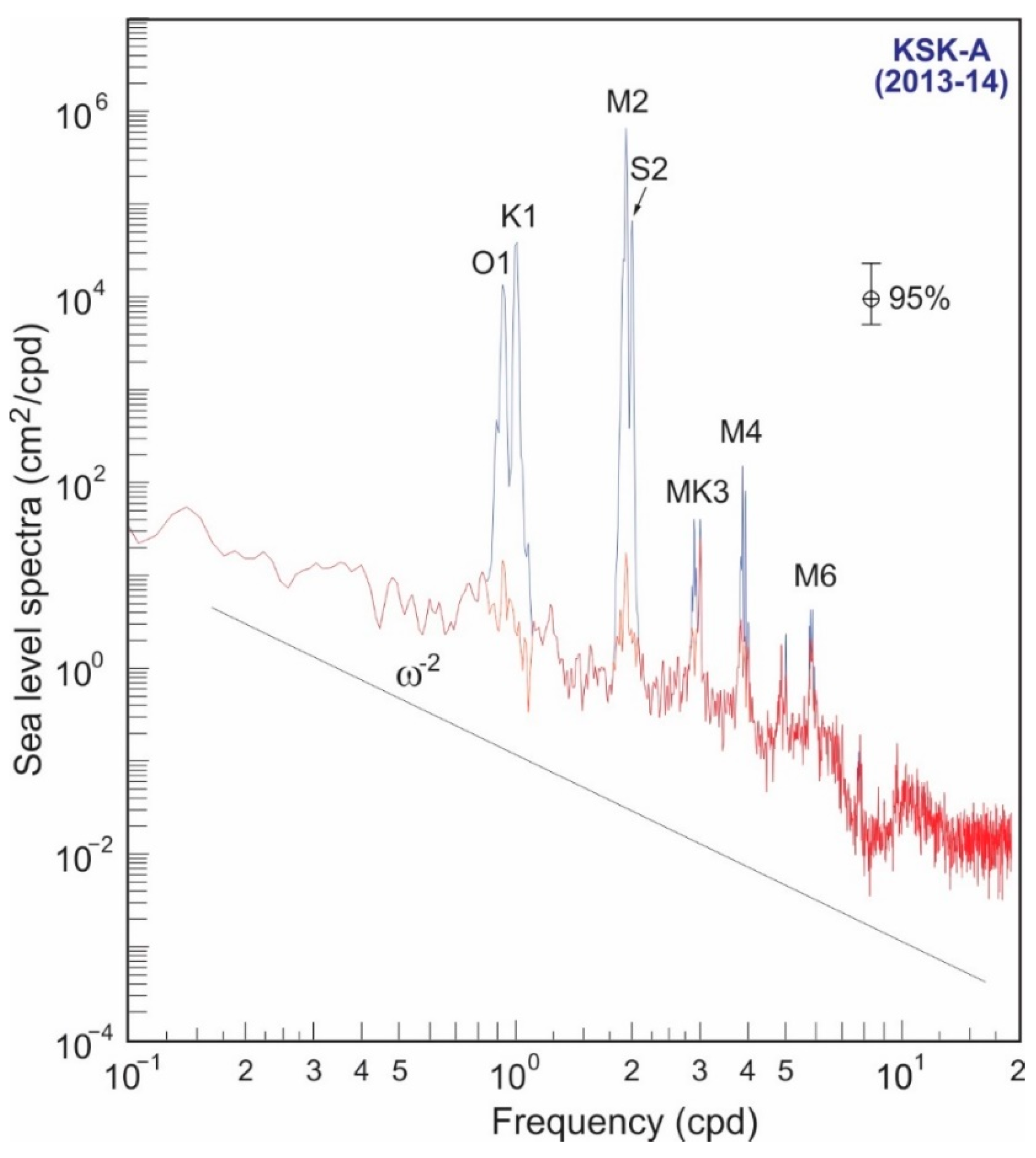
The spectra are “red”; the main energy is concentrated in low frequencies and decreases with increasing frequency according to the power law in the range ${\omega }^{-1.2}-{\omega }^{-1.5}$ (slower than sea level spectra).

(2)

The principal feature of the spectra is a strong and sharp peak at the semidiurnal frequency, indicating the predominant role of the semidiurnal currents in this region. The diurnal peak (K1) is seen at all spectra but 1.0–1.5 orders weaker than the semidiurnal peak. High-frequency tidal peaks M4 and M6 are evident.

(3)

The spectra of clockwise (CW) and counterclockwise (CCW) components in the entire frequency band, including low-frequency and tidal, are almost equal, showing that currents in this region are practically rectilinear (along-channel).

(4)

The “widening” of the semidiurnal peaks near the peak basements (“tidal cusps”) is a clear indication of the influence of internal tidal waves [16]. This effect is especially evident in the uppermost layers (Figure 3).

(5)

The spectral structure in the deeper layers is similar to those in the upper layers, however, the energy level in the entire frequency band is significantly lower. Furthermore, the semidiurnal peak in the deeper layers became much narrower and sharper indicating weaker influence of baroclinic processes on semidiurnal tides in these layers.

3.3. Energy Budget

Guided by the peaks and troughs in the ADCP current velocity spectra, we partitioned the total velocity variance (${\sigma }_0^2$) into four frequency bands $(\Delta {\omega }_j)$: Low- frequency (LF), $\omega$ < 0.8 cpd; diurnal (D), $\omega$ ≈ 0.8 – 1.5 cpd; semidiurnal (SD), $\omega$ ≈ 1.5 – 2.2 cpd; and high-frequency (HF), $\omega$ > 2.2 cpd. For each jth frequency band ($\Delta {\omega }_j$) and for each ADCP bin (depth horizon), we estimated the clockwise, ${\sigma }_j^2(-)$, counterclockwise, ${\sigma }_j^2(+)$, and total, ${\sigma }_j^2(\mathrm{tot})$, variances of the ADCP currents, viz:

$${\sigma }_j^2(-)\hspace{0.17em}=\hspace{0.17em}{\displaystyle {\int }_{\Delta {\omega }_j}\left[S({\omega }^{-})\right]d\omega }$$

$${\sigma }_j^2(+)\hspace{0.17em}=\hspace{0.17em}{\displaystyle {\int }_{\Delta {\omega }_j}\left[S({\omega }^{+})\right]d\omega }$$

(1)

$${\sigma }_j^2(\mathrm{tot})\hspace{0.17em}=\hspace{0.17em}{\sigma }_j^2(-)+{\sigma }_j^2(+)$$

where j = 1, 2, 3, and 4.

As an example, Figure 4 shows bar plots for three ADCP depth levels at Moorings FOC and KSK, Deployment A. In the uppermost layer about 2/3 of the energy of the currents is related to low-frequency (LF) motions and about 1/4 to semidiurnal (SD) motions. These results for the low-frequency motions are in good agreement with those obtained for this region by Wan et al. [5,6]. They indicated that these motions prevail in the uppermost layers and are mostly induced by estuarine circulation and wind-driven currents. The influence of diurnal (D) and high-frequency (HF) motions is insignificant. At depths of 20–50 m, the relative contribution of LF and SD motions is approximately equal, while at lower depths, semidiurnal currents strongly prevail. At depths larger than 250 m semidiurnal currents are responsible for more than 65–70% of the total variance of the observed currents. The general character of currents and their year-to-year (2013–2016) vertical structure/energy budget remained very consistent.

The band-averaged energy estimates of current velocities for specified frequency bands (LF, D, SD, and HF) enabled us to examine the vertical structure of the observed currents. Most of the energy is concentrated in the upper 20 m layer and gradually decreases downward. There is a strong similarity in the vertical structure between various types of motions. This structure is mainly consistent; there are only minor differences between the two moorings. As an example, Figure 5 shows vertical variations of the four components of the observed currents in the upper 40-m layer for moorings FOC and KSK, Deployment C. Below 40 m all four types of motions remain almost uniform and appear to be strongly dominated by barotropic motions. However, as indicated above, in the upper layer there are year-to-year differences in the energy of various components and in the total energy that once again demonstrate the complexity in the prediction of tidal and other types of currents even in a coastal basin, such as Douglas Channel, which has a relatively stable regime of currents.

It is evident that the vertical structure of the four selected frequency bands (LF, D, SD, and HF) strongly depends on the corresponding stratification profiles. As an example, Figure 6 shows three profiles for Mooring FOC and three for KSK. The main changes of these profiles occur in the upper 20-m layer; below this layer, all profiles are very steady and similar for two moorings and for all three deployments. All seasonal and interannual variations take place in the uppermost layer and they are substantial. As was indicated by Stigebrandt [18] and Wan et al. [5], the near-surface stratification in fjords is determined by freshwater input, turbulence, and wind mixing. Intense stratification changes in the upper layer strongly affect the tidal currents creating serious problems for forecasting these currents.

3.4. Harmonic Analysis of Tidal Currents

To understand the essential properties of tidal currents in the Douglas Channel, velocities were harmonically analyzed similarly to sea level (Section 3.1). The harmonic analysis of tidal currents for all instruments, moorings, and deployments was performed independently for U and V components using the least squares method [12,19]. Based on a well-known procedure [14,19], the ellipse parameters were estimated, and tidal ellipses were constructed for four major constituents, O1, K1, M2, and S2 (Figure 7 and Figure 8). Sea level amplitudes for these four harmonics (O1:K1:S2:M2) are roughly related to 18:30:32:100 (Table 3); approximately the same ratios are observed for currents.

The entire character, orientation, direction of rotation, and vertical structure of the S2 currents repeat those of the M2 currents, while the O1 currents match the K1 currents. This means that the M2 and K1 may be considered representatives of the entire groups of SD and D harmonics, respectively. This conclusion is in agreement with Webster [4], who based on analysis of 5-month series of current velocities in Douglas Channel, indicated that “…the semidiurnal barotropic tidal velocities in Douglas Channel were almost directly proportional to the semidiurnal constituents of tidal height”. Both SD and D ellipses are strongly elongated; the FOC currents are mainly oriented in the SW-NE direction, while the KSK currents are almost meridional, both in good agreement with the orientation of the channel in the areas of the moorings (Figure 1). The KSK ellipses are nearly flat; the respective tidal currents are practically rectilinear (back and forth along the same meridional line). At FOC the ellipses have some width and deserve the name of ‘tidal ellipses’.

The spectacular feature of the observed currents is their consistent, natural vertical structure. The changes are gradual, the phases are in agreement and the main properties of tidal ellipses vary from one layer to another one smoothly. In the upper 15–20 m layer at FOC (at all deployments), both D and SD currents are counterclockwise (Figure 7a and Figure 8a,c); at all deeper layers, they are clockwise (Figure 7a). The depth of 15–20 m at FOC is where currents change their sign, and they are almost rectilinear at these depths. The specific feature of the vertical SD structure is its shape with relatively wide “shoulders” (at depths 0–25 m), strong straight “legs” (below 200 m), and relatively narrow “waist” (at 30–100 m). Such structure remains quite consistent for all deployments. It is evident that, except for the upper layer, the SD currents are relatively stable and are dominated by barotropic motions. In contrast to deeper layers, in the upper 25-m layer, there are noticeable differences between the three deployments. In particular, the recorded SD currents during Deployment A were substantially weaker than during Deployments B and C; also, SD current ellipses at KSK in the upper 25-m layer observed during Deployment B were wider and turned clockwise relative to the meridional direction (Figure 8b).

In general, we may assume that the barotropic tidal flow, which is coming into Douglas Channel from Hecate Strait, interacts with the local topography of the channel generating baroclinic SD tidal waves. The main energy of baroclinic tidal motions is concentrated in the upper 25-m layer amplifying these currents. Significant temporal variations in the stratification of the upper mixed layer, stimulated by atmospheric processes, are probably the main reason for the considerable temporal changes in the near-surface tidal currents.

4. Time Variations of Tidal Currents

The along-channel currents strongly prevail in Douglas Channel and, in fact, the “prediction of tidal currents” in this region means, first of all, the prediction of along-channel currents. The question, however, is: “How variable and predictable are these currents?” The reliable prediction of tidal currents is possible only when these currents are stable and highly correlated with sea-level tidal oscillations. To answer this question, we examined temporal (mainly seasonal) variations of tidal currents in the Douglas Channel and used two methods: (a) “multiple-filter technique” and (b) month-by-month harmonic analysis.

Individual current velocity time series were transformed into along-channel (V) and cross-channel (U) components: at KSK the V component was directed almost northward (2º True), whilst at FOC the azimuth of this component was approximately 65º True.

4.1. Frequency-Time Analysis

A “multiple-filter technique” method was used; it is similar to wavelet analysis [12] and is based on narrow-band filters with a Gaussian window that isolates a specific central frequency. Demodulation of the respective time series yields a matrix of amplitudes of wave motions with columns representing time, t, and rows representing frequency, f (the so-called f-t diagrams). The method was found to be very effective to study nonstationary tidal and inertial currents [16,20].

We constructed f-t diagrams for simultaneous series of tidal sea levels and ADCP currents. Figure 9 shows these diagrams for sea level (top plot) and along-channel velocity components at FOC and KSK (one upper and two lower layers), which were recorded during Deployment B (2014–2015). These two sets of f-t diagrams are alike, clearly demonstrating the similarity of dynamical processes, responsible for the formation of the velocity field at these sites and, probably, in the entire Douglas Channel. Sea level oscillations are very steady and regular. Semidiurnal motions are highly dominant in the observed sea levels; diurnal oscillations are second in importance, and third-diurnal and quarter-diurnal tides are also evident. The main feature of the corresponding plots is the fortnightly spring-neap cycle = 1/2 of a synodic month (14.77 solar days) for semidiurnal and quarter-diurnal tides and 1/2 of nodical (lunar declination) month (13.61 solar days) for diurnal tides [17,19].

Time variations of semidiurnal tidal currents in the deeper layers are very similar to those in sea level; the main time variability is determined by the spring-neap cycle. There are no visible seasonal variations of these currents that are typically associated with internal tides. Observations show that stratification changes in the deeper layers are gradual and insignificant and internal tides are weak. Diurnal and high-frequency tidal currents, both in the upper and deeper layers, are noticeable but relatively weak and do not play a marked role in the general dynamics of this region in comparison with semidiurnal currents.

Semidiurnal (SD) tidal currents in the upper layer have a complicated character. These currents are much less regular than SD sea level oscillations or SD currents in deeper layers (Figure 9). It is apparent that these currents are strongly affected by the baroclinic processes. These processes depend on stratification, which is quite variable in the upper layer. Thus, SD tidal currents in this layer are formed under the influence of two opposed processes:

• Regularization: governed by very steady and regular astronomical tidal forcing.
• Randomization: determined by various random factors and, first of all, by changes in stratification and mean currents.

Mean currents and stratification are strongly correlated: changes in stratification influence mean currents, while variations in mean currents affect stratification. Time periods when these two processes were relatively stable appear as consistent and relatively steady SD currents. At these times, the baroclinic SD currents have the character of coherent baroclinic tidal waves that are “phase-locked” to barotropic tidal waves. Fast changes in stratification or the mean currents significantly increase incoherent (random) baroclinic tidal waves [16,21,22]. The periods of “regularization” and “randomization” are evident in the f-t diagrams for the 5-m depth layer in Figure 10 both for KSK and FOC.

To examine better the SD currents in the upper layer we constructed detailed f-t diagrams both for along-channel (V) and cross-channel (U) current velocity components for all three deployments. In general, there are no marked differences in their f-t diagrams, except that the entire Deployment B at both stations was much more energetic (see Section 3.3) than the two other deployments and had the strongest seasonal contrasts (Figure 10). The FOC and KSK f-t diagrams look similar; intense SD currents were observed in the “winter period” (from November 2014 to May 2015), while much weaker SD currents occurred in the summer of 2014 and in June–July 2015.

According to the results of the f-t analysis, ADCP currents recorded at various depths of the upper layer are in good agreement with each other; the observed currents gradually attenuate downward. The upper layers are noisier; the energy of background oscillations, including low-frequency currents, decreases with depth, while the SD tidal currents become more evident. A particular feature apparent in all f-t diagrams is strong vertical bands indicating the entire upper layer is reacting to external forcing, most probably associated with atmospheric processes affecting all of Douglas Channel. Undoubtedly, such irregular variations in the intensity of the SD tidal currents seriously impede the prediction of these currents.

4.2. Tidal Analysis of Monthly Series

Tidal harmonic analysis of the ADCP data gives us another method to examine temporal variations of tidal currents in the upper layer. We used three-year deployments and estimated M2 tidal ellipses month-by-month. The computed M2 ellipses for individual months for moorings FOC and KSK are shown in Figure 11 and Figure 12, respectively. For comparison, we also showed the mean M2 tidal ellipses for the entire observational year.

In general, the results of harmonic analysis of tidal currents are in good agreement with the f-t analysis: vertical changes of these currents are smooth and gradual; however, they are strongly variable in time. The temporal (seasonal) variations of currents are more evident at FOC (Figure 11) than at KSK (Figure 12). In the uppermost layer of 5–15 m, counterclockwise (CCW) motions are, in the northern hemisphere, an indication of the baroclinic motions. These CCW motions become stronger and “thicker” (penetrate to deeper layers) deeper in June–August and weaker and “thinner” in the wintertime (Figure 11). The orientation of ellipses is quite steady, except KSK-B (2014–2015) where during the entire year all the M2 tidal ellipses in the 5–15 m layer are oriented in the NW-SE direction. Month-to-month changes in shapes and sizes of the recorded ellipses at both moorings are gradual and regular; at the same time, the seasonal changes in these ellipses are not consistent and for the same months in different years do not always look alike.

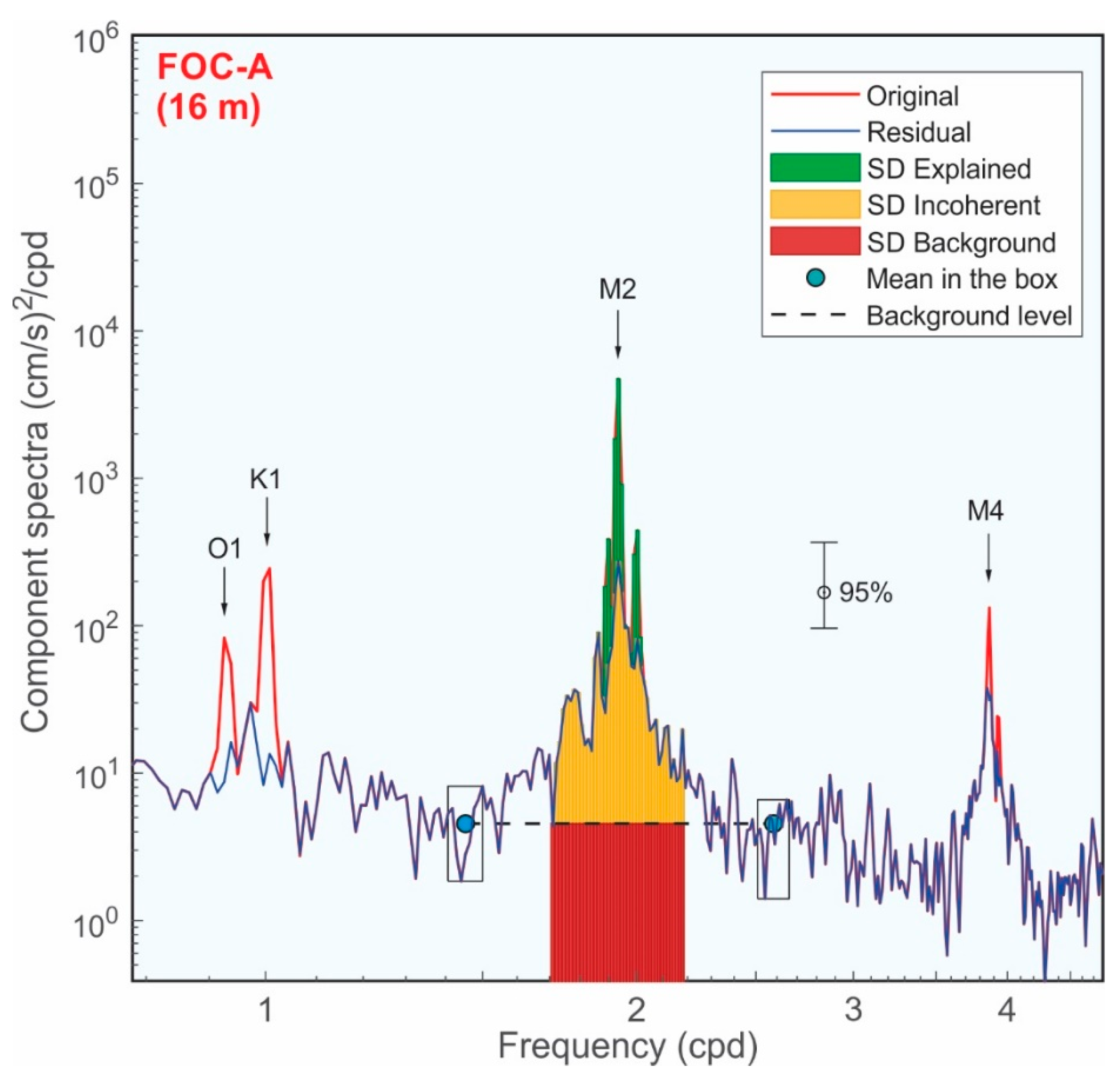
4.3. Energy Decompositions of Semidiurnal Tidal Currents

As was demonstrated by Dushaw et al. [23], Chiswell [21], Cummins et al. [22], and Kulikov et al. [16], a significant part of baroclinic tidal currents in the near-field of the generation area is coherent with the barotropic tide, but the coherence gradually decays with distance from the generation area due to topographic scattering and density variations. Thus both “coherent” (phase-locked) and “incoherent” (random) baroclinic components exist, but their relative contribution depends on the stability of the stratification and the distance from the generation source. The “deterministic” component of tidal currents (associated with barotropic tides and “coherent” baroclinic tides) theoretically can be forecasted, while the “incoherent” (random) component can be predicted only from the “statistical” point of view.

The key problem in separating “coherent” and “incoherent” (i.e., mean and variable) components of baroclinic tidal currents, is to select the averaging period. We used the deployment duration (A, B, and C) as the averaging period and considered only the along-channel SD currents, which are approximately two orders more energetic than the cross-channel SD currents. Based on spectral analysis of yearly time series of the V component of current velocities and harmonic tidal analysis of these series, we separated the observed currents into two parts: deterministic and random.

Figure 13 shows a spectrum of along-channel currents at 16 m depth. The spectrum is formed by two types of processes: (1) continuous background noise, mostly produced by wide-band atmospheric processes and turbulent pulsations, and (2) sharp peaks associated with tidal currents. The tidal peaks are spiky and narrow, corresponding to major tidal harmonics, but have a widening “basement” (cusps) due to the influence of internal tides. Different SD components in Figure 13 are illustrated by different colours. We assume that four major components are responsible for the SD currents in Douglas Channel:

• Barotropic;
• Baroclinic coherent;
• Baroclinic incoherent (random);
• Background noise.

The mean tidal currents estimated over the entire observation period of approximately one year are considered as a “deterministic” part, which is the sum of a barotropic and phase-locked coherent baroclinic component, while the residual currents (after subtraction of hindcasted tidal currents) is a “random” part, which includes an incoherent baroclinic component and non-tidal background noise in the SD frequency band:

$$E_{total}(\Delta {\omega }_{SD})=E_{deter}+\hspace{0.17em}{E}_{random}\hspace{0.17em}=\hspace{0.17em}\hspace{0.17em}\left(E_{barotr}+\hspace{0.17em}{E}_{coher}\right)\hspace{0.17em}+\hspace{0.17em}\left(E_{incoher}+\hspace{0.17em}{E}_{bg}\right)$$

(2)

From the computed spectra we estimated the total energy of currents in the SD band (1.7–2.2 cpd) and by the least squares method from the harmonic analysis, we calculated mean tidal currents. In this way, we divided the entire energy of SD currents into two parts: “explained” and “residual” (Figure 13). Moreover, the spectral estimates help us roughly evaluate the background noise contribution to the SD currents (Figure 11). The difference between the residual and background noise is the “incoherent baroclinic” component. In this way, for each ADCP layer, we separated the entire SD energy into three partitions: “explained” (deterministic), “incoherent” (random), and “background”; the respective results for both layers and all three deployments are shown in Figure 14a. In principle, the top-to-bottom examination of the ADCP currents enables us to isolate and distinguish the barotropic component of the SD currents, i.e., to separate the “explained” part into two individual components: “barotropic” and “coherent baroclinic”. However, this is out of the scope of the present study.

Figure 14a demonstrates that most of the SD energy can be explained. Our results also show that the percentage of “unexplained” (i.e., “residual”) energy is much higher in the uppermost layer than in the lower layers. We can use our estimates for each ADCP layer to calculate the total energy of the SD currents ($\widehat{E}$_total) within the upper (Δz_up) and lower (Δz_low) layers, as well as the integral ($\widehat{E}$_j) and relative ($\widehat{E}$_j^rel) estimates of the three energy partitions within these layers:

$$\widehat{E}{}_{total}={{\int }_{{∆z}_{up,low}}^{}E}_{total}\left(z\right)dz;\widehat{E}{}_j={{\int }_{{∆z}_{up,low}}^{}E}_j\left(z\right)dz;\widehat{E}{}_j{}^{rel} (\widehat{E}{}_j/{\widehat{E}}_{total})·100\%; j=1,2,3.$$

(3)

Relative estimates of the “explained”, “incoherent” and “background” components of along-channel currents are indicated in Figure 14a,b. The results for three deployments are averaged and summarized in

Table 4. Mean along-channel current velocity components at Moorings KSK and FOC averaged over three deployments: A (2013–2014), B (2014–2015), and C (2015–2016).

Component	FOC		KSK
	Upper (cm/s)2	Lower (cm/s)2	Upper (cm/s)2	Lower (cm/s)2
Total	102.7 (100%)	76.4 (100%)	96.1 (100%)	49.9 (100%)
Explained	80.4 (78.3%)	70.1 (91.7%)	85.4 (88.9%)	47.3 (94.8%)
Incoherent	19.8 (19.3%)	5.6 (7.4%)	8.7 (9.0%)	2.3 (4.6%)
Background	2.5 (2.4%)	0.7 (0.9%)	2.0 (2.1%)	0.3 (0.6%)

. These results enable us to make certain conclusions about the character of the observed ADCP currents:

(1)

The total variance of the recorded along-channel SD currents at moorings FOC and KSK in the upper layer was approximately equal: ~100 (cm/s)²; in the lower layer, SD currents at FOC were much more energetic than at KSK: ~75 and 50 (cm/s)², respectively.

(2)

In the upper layer, about 90% at KSK and 78% at FOC of the total energy of SD currents are related to the “explained” component (i.e., to barotropic and baroclinic coherent). In the lower layer, these values are 95% and 92%, respectively.

(3)

More “explained” energy is observed at KSK than at FOC. It appears that the reason for this difference (~12% in the upper layer and ~3% in the lower layer) is the nearness of KSK to the entrance of Douglas Channel, i.e., to a hypothetical source area of baroclinic SD waves. The “randomization” of the coherent SD tidal component on its way from KSK to FOC may cause the decrease of the “explained” energy partition along the channel.

(4)

The highest percentage of unexplained (random) energy of SD tidal currents is related to the uppermost 10-m layer, i.e., to the layer with the strongest stratification variations (see Figure 7).

(5)

The strong dominance of the “explained” energy in the lower layer (92–95%) is because the SD currents in this layer are almost barotropic.

(6)

The contribution of background currents in the total energy of the SD currents is small: 2–2.5% in the upper layer and 0.6–0.9% in the lower layer.

5. Discussion

Our study is based on the analysis of three years of ocean currents and subsurface pressure data at two stations, KSK and FOC, which are located along the axis of Douglas Channel approximately 30 km apart. The tidal component of the sea level variability, estimated from bottom pressure measurements, was found to be very consistent; the tidal constants estimated from different yearly deployments were almost the same. For major harmonics, the differences in independently evaluated constants from the three deployments were less than 0.2–0.3%. The tidal constants estimated for KSK and FOC were also in close agreement with those computed for CHS tide gauges located at Kitimat and Hartley Bay.

In contrast to the prediction of tidal sea level oscillations, the prediction of tidal currents is always a challenge. Tidal sea levels are almost entirely deterministic; they can be calculated for hundreds of years with very high precision. Tidal currents are substantially influenced by changes in the stratification and mean currents and, as a result, are much more variable and less predictable. We have used the term “deterministic” to denote the sum of barotropic and phase-locked coherent baroclinic SD tidal components. The “coherent” baroclinic component corresponds to the mean characteristics of stratification and long-period currents within a specific period of time, in our case within the deployment periods. However, these “mean” characteristics vary from year to year causing corresponding variations of baroclinic tides. The higher the contribution of barotropic tidal currents to the total energy of the recorded SD currents, the steadier are stratification and mean currents, and the more precisely we can predict tidal currents.

In the previous section, we hindcasted tidal currents, i.e., estimated the “deterministic” component of current velocities based on the results of tidal analyses of the same series. In this way, we could split the entire SD tidal energy into “explained” and “residual” and estimate mean tidal currents at all ADCP depth layers for each specific deployment. The important point is that the entire algorithm of the least squares method is directed to maximize the explained variance and minimize the residual variance. This means that it is the best possible prediction that could be achieved for this particular series with this set of harmonics. The principal question is: How close can we approach this limit if we use tidal constants estimated from an independent time series?

To evaluate the effectiveness of the forecast of the SD tidal currents in Douglas Channel and to validate our results, we used tidal constants for each station, layer, and deployment. Then the set of corresponding tidal constants estimated from one deployment was used to predict the tidal currents in the same layer for the two other deployments. The results for individual layers are shown in Figure 14a, while the general estimates integrated within the upper (Δz_up) and lower (Δz_low) layers are shown in Figure 14b.

Naturally, the “forecasted” energy is slightly smaller than the self-predicted “explained” energy, while the residual (“unexplained”) energy is larger. To illustrate this, we constructed

Table 5. The mean percentage of explained SD along-channel current velocity variance at Moorings KSK and FOC, Deployments A, B, and C estimated for the upper and lower integral layers based on tidal constants (A_j, B_j, and C_j) calculated from the same deployment (diagonal matrix elements denoted by bold) and from two other deployments.

VHC	FOC						KSK
	Upper			Lower			Upper			Lower
	A	B	C	A	B	C	A	B	C	A	B	C
Aj	77.3	73.6	64.3	91.2	84.4	85.4	92.7	84.2	79.6	-	-	-
Bj	70.4	82.6	71.0	79.2	93.2	89.4	85.4	90.6	82.2	-	95.4	92.9
Cj	55.0	60.7	74.5	86.8	88.7	91.0	88.8	86.6	86.0	-	92.9	94.1

which includes four matrices (two moorings and two layers) of the relative percentage of computed variance ($\widehat{E}$_j^rel). The diagonal elements of each matrix show the results of hindcasting (i.e., the percentage of “explained” variance for each mooring, deployment, and integral layer), while other matrix elements show the results of forecasting. In general, the difference is not large, and the results look encouraging. At KSK, located closer to the entrance of Douglas Channel, from 80 to 89% of the total energy of the SD tidal currents in the upper layer can be forecasted; in the lower layer these numbers are even larger: 89 to 93%. In the lower layer at FOC, the fraction that can be forecasted is from 79 to 89%; i.e., practically the same as at KSK. However, in the upper FOC layer, this fraction is distinctly lower, from 55 to 70%.

In general, our results show that tidal currents in the lower layer are dominated by barotropic motions; they are functionally related to tidal sea levels and, consequently, are steady, consistent, and predictable. The amplitudes of barotropic M2 currents at KSK and FOC stations are ~10–12 cm/s, where the “lower layer” is considered as everything below ~50 m from the surface. Table 5 indicates that in this layer we can forecast 91 to 95% of the semidiurnal (SD) tidal energy at KSK and 85 to 91% at FOC based on tidal constants computed from any of the 3 years.

The situation in the upper layer is more complicated. Here we define the “upper layer” as everything above ~50 m, however, the strongest effects are in the upper 10 m, i.e., in the layer of the strongest stratification changes. The difference between the ‘total’ currents in the upper layer and the “explained” currents in the lower layer shows that 35–55% of the total energy of semidiurnal currents in the upper layer is associated with baroclinic motions (Table 4), where we have assumed that the lower layer is purely barotropic. We can use tidal analysis to estimate and predict the “mean baroclinic SD currents” (i.e., that part that is “coherent” or “phase-locked” with the barotropic component), but cannot predict the “incoherent” component. Thus, the higher the percentage of the “explained” component, the higher the quality of our forecasts of tidal currents for the upper layer.

Our results (Table 4 and Table 5) demonstrate that Station FOC has substantially more “random SD tidal energy” in the upper layer than Station KSK (17–24% and 6–12%, respectively), while for the “coherent SD energy” the situation is opposite. A number of studies of internal tidal waves over the last two decades [16,21,22,23] indicate that typically coherent baroclinic waves decrease rapidly with distance from the source; vice versa, the relative contribution of incoherent baroclinic waves increases with distance from the source, which is typically a region of intense interaction of the barotropic tidal flow with topography. It appears that the source area is located south of KSK, i.e., near the entrance to Douglas Channel. The increase in incoherent energy toward the channel head can also be related to the topographic scattering of propagating coherent baroclinic waves along the channel (“randomization of phase-locked baroclinic tides”).

There is also another important problem in forecasting SD tidal currents: The variations of the coherent baroclinic component itself. As was emphasized above, this component is not something precisely determined and uniform, but rather a component corresponding to certain mean stratification characteristics and long-period currents within a specific period of time (“reference period”). In the present study, we selected this period to be the deployment period, i.e., approximately one year. Variations of “mean characteristics” within a year and between different years cause variations of baroclinic tidal currents and limit the quality of the tidal current prediction.

However, on the whole, the results of our study look encouraging: In the upper layer at KSK and FOC moorings, about 70–80% of the total variance of along-channel SD tidal currents can be forecasted. The typical speed of these currents is ±10–15 cm/s, while “random” (unpredictable) SD currents may add only 3–5 cm/s to these values.

All these results do not take into account seasonal variations of tidal currents. In fact, we tried to use monthly reference periods to determine a specific set of tidal constants for this particular month (“January”, “February”, etc.), however, the results were disappointing: We found that current forecasting based on yearly tidal computations gives much better and more consistent results than those based on individual months.

We have used the word ‘prediction’ in the sense of statistical prediction (or tidal analysis). Coastal ocean circulation models are an alternative prediction tool. The ‘explained’ component of the semidiurnal currents (barotropic plus coherent baroclinic) should be viewed as an upper bound on the predictability using such models. Achieving this upper bound will require accurate simulation of the surface stratification and modes 2 and 3 of the internal wave structure; these are both demanding tasks given the thin stratified surface layer (10–20 m) and the small Rossby radii for these modes (2–3 km) in Douglas Channel. Therefore, numerical models of the currents are unlikely to simulate all of the ‘explained’ components of the semidiurnal currents in the foreseeable future; there will always be semidiurnal currents in the time series of the difference between modelled and observed currents.

6. Conclusions

Spectral, wavelet, and harmonic analysis of measured currents throughout the upper (40-m) and lower (50–358 m) water columns were used to examine the variability and predictability of tidal currents based on three years of current velocity data collected at two moorings, FOC and KSK, located 30 km apart, within Douglas Channel, British Columbia. The analysis showed the predominant contribution of semidiurnal (SD) tidal currents in the energy budget of the observed current velocities. In the upper layer, there was considerable seasonal and interannual variability of SD currents caused wind and density flows, while in the deeper layer, they were relatively steady and consistent and appear to be mostly barotropic.

To assess the potential for an effective forecast of the tidal currents in the region we developed a methodology, based on spectral and harmonic analyses, to partition the current energy into three major components: barotropic, coherent baroclinic, and random baroclinic. The predictability of the currents depends on the relative contribution and stability of the first two components—the ‘deterministic’ or ‘explained’ component. At KSK about 90% of the total energy of SD currents in the upper layer is related to the “explained” component, whereas at FOC it reduces to 78%. In the lower layer, these values are 95% and 92%, respectively. These results were confirmed by using tidal constants estimated for one year to predict the SD currents for the two other years. At the mooring closer to the entrance of Douglas Channel (KSK), 80 to 89% of the SD energy in the upper layer and 89–93% in the lower can be forecasted using standard tidal analysis techniques, while closer to the channel head (FOC), these numbers are smaller: 55–70% and 79–89%, respectively. This is attributed to the more variable stratification and mean currents at the head of the fjord.

The methodology can be used widely to place bounds on how predictable the tidal currents are at a particular location and to place upper bounds on what can be expected from numerical model simulations of tidal currents.

References

1. Macdonald, R.W.A. Proceedings of a Workshop on the Kitimat Marine Environment; Canadian Technical Report of Hydrography and Ocean Sciences; Fisheries and Oceans Canada: Vancouver, BC, Canada, 1983; Volume 18, v+218p. Available online: http://waves-vagues.dfo-mpo.gc.ca/Library/52404-1.pdf (accessed on 1 November 2021).
2. Shaw, J.; Stacey, C.D.; Wu, Y.; Lintern, D.G. Anatomy of the Kitimat fiord system, British Columbia. Geomorphology 2017, 293, 108–129. [Google Scholar] [CrossRef]
3. Huggett, W.; Wigen, S. Surface currents in the approaches to Kitimat. In Proceedings of a Workshop on the Kitimat Marine Environment; Macdonald, R.W., Ed.; Canadian Technical Report of Hydrography and Ocean Sciences; Fisheries and Oceans Canada: Sidney, BC, Canada, 1983; Volume 18, pp. 34–65. [Google Scholar]
4. Webster, I. The baroclinicity of the semi-diurnal tidal currents in Douglas Channel, B.C. In Proceedings of a Workshop on the Kitimat Marine Environment; Macdonald, R.W., Ed.; Canadian Technical Report of Hydrography and Ocean Sciences; Fisheries and Oceans Canada: Sidney, BC, Canada, 1983; Volume 18, pp. 14–33. [Google Scholar]
5. Wan, D.; Hannah, C.G.; Foreman, M.G.G.; Dosso, S. Subtidal circulation in a deep-silled fjord: Douglas Channel, British Columbia. J. Geoph. Res. Oceans 2017, 122, 4163–4182. [Google Scholar] [CrossRef]
6. Wan, D.; Hannah, C.G.; Cummins, P.F.; Foreman, M.G.G.; Dosso, S.E. Wind-driven currents in a “wide” narrow channel, with application to Douglas Channel, BC. J. Geoph. Res.-Oceans 2022, 127, e2021JC017887. [Google Scholar] [CrossRef]
7. Wright, C.A.; Vagle, S.; Hannah, C.; Johannessen, S.J. Physical, Chemical and Biological Oceanographic Data Collected in Douglas Channel and the Approaches to Kitimat, June 2013–July 2014; Canadian Data Report of Hydrography and Ocean Sciences; Fisheries and Oceans Canada: Sidney, BC, Canada, 2015; Volume 196, viii+66pp. Available online: http://www.dfo-mpo.gc.ca/Library/359327_pt1.pdf (accessed on 1 November 2021).
8. Wright, C.A.; Vagle, S.; Hannah, C.; Johannessen, S.J.; Spear, D.; Wan, D. Physical, Chemical and Biological Oceanographic Data Collected in Douglas Channel and the Approaches to Kitimat, October 2014–July 2015; Canadian Data Report of Hydrography and Ocean Sciences; Fisheries and Oceans Canada: Sidney, BC, Canada, 2016; Volume 200, viii+74pp.
9. Wright, C.A.; Vagle, S.; Hannah, C.; Johannessen, S.J.; Spear, D.; Wan, D. Physical, Chemical and Biological Oceanographic Data Collected in Douglas Channel and the Approaches to Kitimat, October 2015–July 2016; Canadian Data Report of Hydrography and Ocean Sciences; Fisheries and Oceans Canada: Sidney, BC, Canada, 2017; Volume 202, x+139pp, Available online: http://waves-vagues.dfo-mpo.gc.ca/Library/40645186.pdf (accessed on 1 November 2021).
10. Gonella, J. A rotary-component method for analyzing meteorological and oceanographical vector time-series. Deep-Sea Res. 1972, 19, 833–846. [Google Scholar]
11. Mooers, C.N.K. A technique for the cross spectrum analysis of pairs of complex-valued time series, with emphasis on properties of polarized components and rotational variants. Deep Sea Res. 1973, 20, 1129–1141. [Google Scholar] [CrossRef]
12. Thomson, R.E.; Emery, W.J. Data Analysis Methods in Physical Oceanology, 3rd ed.; Elsevier: New York, NY, USA, 2014; 716p. [Google Scholar]
13. Foreman, M.G.G. Manual for Tidal Heights. Analysis and Prediction; Pacific Marine Science Report 77-10; Institute of Ocean Sciences: Sidney, BC, Canada, 1977; (revised 2004); 58p, Available online: http://www-sci.pac.dfo-mpo.gc.ca/osap/publ/online/currents2004.pdf (accessed on 1 November 2021).
14. Foreman, M.G.G. Manual for Tidal Currents Analysis and Prediction; Pacific Marine Science Report 78-6; Institute of Ocean Sciences, Patricia Bay: Sidney, BC, Canada, 1978; (2004 revision); 57p, Available online: http://www.pac.dfo-mpo.gc.ca/sci/osap/projects/tidpack/tidpacke.htm (accessed on 1 November 2021).
15. Pawlowicz, R.; Beardsley, B.; Lentz, S. Classical tidal harmonic analysis including error estimates in MATLAB using T_TIDE. Comp. Geosc. 2002, 27, 929–937. [Google Scholar] [CrossRef]
16. Kulikov, E.A.; Rabinovich, A.B.; Carmack, E.C. Barotropic and baroclinic tidal currents on the Mackenzie shelf break in the southeastern Beaufort Sea. J. Geoph. Res. 2004, 109, C05020. [Google Scholar] [CrossRef]
17. Pugh, D.; Woodworth, P. Sea-Level Science: Understanding Tides, Surges, Tsunamis and Mean Sea-Level Changes; Cambridge Univ. Press.: Cambridge, UK, 2014; 395p. [Google Scholar]
18. Stigebrandt, A. Hydrodynamics and circulation of fjords. In Encyclopedia of Lakes and Reservoirs; Lars Bengtsson, R.W.F., Herschy, R.W., Eds.; Springer: New York, NY, USA, 2012; pp. 327–344. [Google Scholar] [CrossRef]
19. Pugh, D.T. Tides, Surges and Mean Sea-Level; John Wiley: Hoboken, NJ, USA, 1987; 472p. [Google Scholar]
20. Zaytsev, O.; Rabinovich, A.B.; Thomson, R.E.; Silverberg, N. Intense diurnal surface currents in the Bay of La Paz, Mexico. Cont. Shelf Res. 2010, 30, 608–619. [Google Scholar] [CrossRef]
21. Chiswell, S.M. Energy levels, phase, and amplitude modulation of the baroclinic tide off Hawaii. J. Phys. Oceanogr. 2002, 32, 2640–2651. [Google Scholar] [CrossRef]
22. Cummins, P.F.; Cherniawsky, J.Y.; Foreman, M.G.G. North Pacific internal tides from the Aleutian Ridge: Observations and modelling. J. Mar. Res. 2001, 59, 167–191. [Google Scholar] [CrossRef]
23. Dushaw, B.D.; Cornuelle, B.D.; Worcester, P.F.; Howe, B.M.; Luther, D.S. Barotropic and baroclinic tides in the central North Pacific Ocean determined from long-range reciprocal acoustic transmissions. J. Phys. Oceanogr. 1995, 25, 631–647. [Google Scholar] [CrossRef]
Figure 1. The region of study and the location of moorings FOC and KSK in Douglas Channel (red circles) and permanent Canadian Hydrographic Service (CHS) tide gauge Kitimat and Hartley Bay (green squares).
Water 15 02441 g001
Figure 2. Spectra of the original (blue line) and de-tided (red line) bottom pressure records at Mooring KSK in Douglas Channel, Deployment A (3 July 2013–3 July 2014). Spectral peaks of major tidal harmonics are indicated.
Water 15 02441 g002
Figure 3. Rotary spectra of currents were recorded at four ADCP depths: 10, 36, 274, and 358 m at Mooring FOC, Deployment A-upper (2013–2014). The red (−) and blue (+) curves are related to the CW and CCW rotary spectra, respectively. The K1, M2, M4, and M6 tidal peaks are denoted, and the power law ω−1.5 is shown by a straight line.
Water 15 02441 g003
Figure 4. Bar plots (band averaged energy) for the CW (S-) and CCW (S+) rotary spectra at Moorings KSK and FOC, Deployment A (2013–2014). The constructed bars are related to depths 10, 24, and 36 m for FOC and 6, 26, and 46 m for KSK. Bands are low-frequency (LF), diurnal (D), semidiurnal (SD), and high-frequency (HF).
Water 15 02441 g004
Figure 5. Vertical profiles of the CW (S−), CCW (S+), and total (Stot) of band-averaged energy of current velocities for four frequency bands: Low-frequency (LF), diurnal (D), semidiurnal (SD), and high-frequency (HF) at Moorings FOC and KSK, Deployment C (2015–2016).
Water 15 02441 g005
Figure 6. Vertical density profiles at moorings FOC and KSK for three selected spring (blue curves) and summer (red curves) observation periods were estimated based on 2013–2014 cruise CTD data.
Water 15 02441 g006
Figure 7. Tidal ellipses for four major diurnal (K1 and O1) and semi-diurnal (M2 andS2) tidal harmonics for moorings (a) FOC (two ADCP instruments, up and down, and two Aquadopps) and (b) KSK (one ADCP up and two Aquadopps), Deployment A (2013–2014). Red ellipses are clockwise (−), and blue ellipses are counterclockwise (+).
Water 15 02441 g007
Figure 8. Tidal ellipses for four major diurnal (K1 and O1) and semi-diurnal (M2 and S2) tidal harmonics in the upper 52-m layer for moorings (a) FOC (ADCP up and Aquadopp) and (b) KSK (ADCP up), Deployment B (2014–2015); and (c) FOC (ADCP up) and (d) KSK (ADCP up), Deployment C (2015–2016). Red ellipses are clockwise (−), and blue ellipses are counterclockwise (+).
Water 15 02441 g008
Figure 9. Frequency-time plots (f-t diagrams) for sea-levels (upper plot) and along-channel (V) currents at depths 5 m (upper ADCP), 263 and 359 m at Mooring FOC, and 226 and 331 m at Mooring KSK (lower ADCP) for the second (B) deployment of the instruments (2014–2015). The frequency range is 0.4–6.0 cpd (periods from 2.5 days to 4 h).
Water 15 02441 g009
Figure 10. Frequency-time plots (f-t diagrams) for along-channel (V) and cross-channel (U) currents at four depths in the upper layer for the second (B) deployment of the instruments (2014–2015) at Moorings (a) FOC and (b) KSK. The frequency range is 0.4–6.0 cpd (periods from 2.5 days to 4 h. Note that the amplitude scale for V and U is different.
Water 15 02441 g010
Figure 11. The M2 tidal ellipses in the upper layer of Mooring FOC, Deployments A, B, and C.
Water 15 02441 g011
Figure 12. The same as in Figure 13 but for Mooring KSK.
Water 15 02441 g012
Figure 13. Tidal spectra of along-channel currents at Station FOC, Deployment A, depth 16 m. Original and residual (de-tided) spectra; major tidal harmonics are indicated; the dashed horizontal red line indicates the background noise level for the SD frequency estimated based on the non-tidal spectra averaged inside the shown boxes.
Water 15 02441 g013
Figure 14. (a) Along-channel ADCP current variances in the SD frequency band for Deployments A, B, and C. The colours denote contributions from different current components to the total variance at each layer: Green is “explained” (barotropic + baroclinic coherent), orange is baroclinic random (incoherent), and red is background noise. Integral estimates of these components for upper and lower layers are indicated. “Predicted” residual variances based on independent analysis of tidal currents from the two other deployments are also shown as “Residual (B) and (C)” for Deployment A, “(A) and (C)” for Deployment B and “(A) and (B)” for Deployment C. (b) Mean along-channel ADCP current variances in the SD frequency band for Deployments A, B and C averaged over the entire layer (upper or lower). The meaning of colours is the same as in (a). The summary variances of these three components for each mooring and deployment within the upper (Δzup) and lower (Δzlow) layers were estimated from Equation (3). The percentages of “explained” and predicted variances (based on the two other deployments) are indicated.
Water 15 02441 g014