Abstract
The extent to which the South-to-North Water Transfer Project has influenced the trend in water storage deficit in the North China Plain since its official opening in late 2014 has not been systematically assessed. We evaluated the changes in terrestrial water storage (TWS) in the North China Plain based on the Gravity Recovery and Climate Experiment (GRACE) and GRACE Follow-on (GRACE-FO) long-term gravity satellite observations from 2002 to 2022, using spherical harmonic (SH) solutions from the Center for Space Research (CSR), GeoForschungsZentrum (GFZ), Jet Propulsion Laboratory (JPL), and Mass Concentration (Mascon) solutions from CSR, Goddard Space Flight Center (GSFC), JPL, and compared with the South-to-North Water Transfer water supply (13.91 Gt/a). The CSR-SH solution that best matched the water supply was selected, and it was found that the rate of change in TWS in the North China Plain from 2002 to 2015 was (−8.48 ± 1.87) Gt/a, and the rate of change from 2015 to 2019 increased significantly to (5.44 ± 4.87) Gt/a, indicating that the TWS in the plain changed from deficit to gain. The South-to-North Water Transfer Project has played a positive role in significantly improving the water stress situation in North China. Simultaneously, by comparing the inversions of six time-varying gravity field models (CSR-SH, GFZ-SH, JPL-SH, CSR-Mascon, GSFC-Mascon, and JPL-Mascon) with the South-to-North Water Transfer water supply and measured groundwater well data, and by calculating the uncertainty using the ‘three-cornered hat method’ (TCH), a comprehensive comparison is made to conclude that the CSR-SH model is most effective with a minimum difference of 0.01 Gt/a from the annual water supply, a minimum difference of 0.04 Gt/a from the measured well data, and a small uncertainty of 3.04 cm. This study reveals the important impact of the South-to-North Water Transfer Project on TWS in the North China Plain, which is of reference value for water resource management decisions in China.
1. Introduction
Located in the east of China, the North China Plain is the second largest plain in China. Due to the dense population and uneven distribution of water resources, people rely heavily on groundwater as a source of water supply, and water supply and demand are in sharp contrast. However, the long-term exploitation of groundwater has led to a series of environmental problems such as the formation of surface funnels, the deterioration of water quality, and ecological degradation, seriously affecting socioeconomic development and human life [1].
To alleviate the lack of water in North China, China has launched the South-to-North Water Transfer Project, the world’s largest water transfer project, to deliver water to North China from the Yangtze River. Since the middle route of the project was completed, it has added a large amount of water resources to the North China Plain and enabled a significant increase in the water supply security capacity. The study of the spatial distribution characteristics and temporal variation patterns of land water storage changes in the North China Plain before and after the South-to-North Water Transfer is of major scientific and social relevance for the region’s sustainable use of water resources.
Many scholars have conducted studies on the changes in water reserves in water-receiving areas after the South-to-North Water Transfer Project. Feng et al. [2] used Gravity Recovery and Climate Experiment (GRACE) observations, combined with hydrological models and actual well measurements, to calculate the groundwater storage deficit rate in the North China Plain from 2003 to 2010 to be about 2.2 cm/a. Zhao’s [3] analysis of the groundwater deficit rate in North China from 2004 to 2016 and from 2013 to 2016 using various GRACE products revealed that the deficit rate increased after 2013 as precipitation fell. Li et al. [4] used GRACE/GRACE Follow-on (GRACE-FO) observations and hydrological model data to analyze the spatial and temporal variability of water storage in the North China Plain from 2004 to 2019. Zhang et al. [5] used GRACE satellite data to invert the changes in groundwater storage in the North China Plain from 2003 to 2015 and validated them with monitoring well data. He [6] inferred the spatial and temporal changes in water storage in the North China Plain from 2002 to 2016 and combined them with GLDAS hydrological model data, Mascon data and GPCC precipitation data for comparative analysis. However, the results obtained by different scholars using different observations and data processing methods vary, and they focus more on the changes in groundwater storage. As for whether and to what extent the South–North Water Transfer Project mitigates the decreasing trend in water reserve in North China, there are fewer assessment reports, the time span is short, and the analysis of the important role of the South–North Water Transfer Project for the North China Plain is incomplete. Additionally, there is a lack of quantitative analysis of how human activity and climate change affect regional water storage. In addition, different scholars have only used a single time-varying gravity field model for inversion, and there is no cross-sectional comparison of the effectiveness of various GRACE/GRACE-FO spherical harmonic (SH) coefficients and mass concentration (Mascon) products for the inversion of water storage changes in the North China Plain.
In this study, the GRACE/GRACE-FO SH coefficient products and Mascon products are used to invert the trends of water reserve in the North China Plain before and after the project for the time periods 2002–2014 and 2015–2022 to discuss the influence of the South-to-North Water Transfer Project on the changes in water reserves in the plain. In addition, we compare the results of SH and Mascon inversion of water reserves with the project’s water supply and the measured groundwater well data, and use the ‘three-cornered hat method’ (TCH) to calculate the uncertainty. Finally, we comprehensively evaluate the effect of various time-varying gravity field models on explaining the influence of the South-to-North Water Transfer Project on water reserves in the North China Plain.
2. Materials and Methods
2.1. Study Area
The North China Plain borders the Yellow Sea and Bohai Sea in the east, reaches Taihang Mountain in the west, starts from Yanshan Mountain in the north, and approaches the Yellow River in the south, with a geographical location of 114°~121° E and 32°~40° N. The terrain is low and flat, with an altitude of less than 100 m. The main component of the North China Plain is the Yellow Huaihai Plain, which has a temperate monsoon climate with high temperatures and rainfall in summer and cold winters with large interannual temperature differences. The study area includes all plain areas of Beijing, Tianjin. and Hebei Province, and plain areas north of the Yellow River in Henan and Shandong Province (Figure 1). The overall area of the study area is approximately 127,000 square kilometers, exceeding 63,000 square kilometers, and GRACE/GRACE-FO terrestrial water storage anomaly (TWSA) calculates the equivalent water height within the study area to an accuracy of 2 cm.
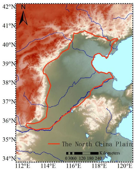
Figure 1.
Geographical location of the North China Plain.
By using the Beijing–Hangzhou Grand Canal and its parallel watercourses to enter Dongping Lake and divide the water in two ways: one to the north to Tianjin and the other to the east to the Jiaodong region, the eastern route of the South-to-North Water Diversion Project is intended to divert water from the main stream of the Yangtze River close to Yangzhou in Jiangsu Province. The first phase of the middle route of the project officially opened for the public on 12 December 2014. Starting from Danjiangkou Reservoir, water is released through the first gate of Taocha Canal, flowing through Henan and Hebei, and past the Xiheishan Bleeder in Baoding City, heading north to Beijing, and flowing east to Tianjin.
2.2. Study Data
2.2.1. GRACE/GRACE-Follow Data
- (1)
- Spherical Harmonic (SH) Products
In this study, GRACE/GRACE-FO satellite’s RL06 monthly time-varying gravity field released by Center for Space Research (CSR), GeoForschungsZentrum (GFZ), and the Jet Propulsion Laboratory (JPL) were used to calculate and analyze water reserves in the North China Plain.
The RL06 data were preprocessed as follows: We applied the DDK3 filtering for smoothing, included the degree-1 coefficients with geocentric corrections provided by Swenson et al. [7] in TN13 based on atmospheric ocean model and high-order GRACE data, used satellite laser ranging (SLR) estimates to replace all GRACE/GRACE-FO second-order term spherical harmonic coefficients [8], replaced the C30 coefficients in GRACE-FO with the SLR solutions in TN14, and used the ICE6G-D model to modify the GIA effect. In order to compare and analyze the data of Mascon products, the average value from 2004 to 2009 was deducted.
- (2)
- Mascon Products
For the Mascon products, we used the GRACE/GRACE-FO RL06 v02 Mascon from CSR [9], the RL06 v02 Mascon from Goddard Space Flight Center (GSFC) [10], and the RL06 v02 Mascon from JPL (CRI-filtered) [11]. The recommended gain factors were applied for the JPL Mascon. GRACE Mascon series products use regularization methods in data processing to calculate changes in terrestrial water storage (TWS) directly from Level1B data, which overcome the need for filtering and smoothing of spherical harmonic coefficient products, thus effectively reducing the north–south band error noise and correcting the leakage error. The GRACE/GRACE-FO data we used are the TWSA relative to the average baseline from 2004 to 2009, and the results are represented by equivalent water height (EWH).
2.2.2. Hydrologic Data
- (1)
- GLDAS Hydrologic Model Data
In this study, Noah data under the Global Land Data Assimilation System (GLDAS) hydrological model data (hereafter referred to as GLDAS_Noah model) were used [12]. This model has a spatial resolution of and uses solar radiation and rainfall observations as input parameters. Four layers of soil water (0~0.1 m, 0.1~0.4 m, 0.4~1 m and 1~2 m) provided by the GLDAS_Noah model were used to calculate land water changes in the North China Plain. The maximum seasonal amplitude of gravity change caused by canopy water change and snow cover change was 5 mm and 4 mm, respectively, but it was still an order of magnitude smaller than the uncertainty of GRACE (2 cm), so the changes in both could be ignored.
- (2)
- Groundwater Logging Data
Groundwater logging data [13] are the groundwater level observation data of the North China Plain, spanning January 2005 to December 2018, with observation intervals of 1 month and water levels in m. The groundwater level data of the North China Plain are in situ observations. The groundwater level data were postprocessed using distance leveling and included monthly scale water level spatial data from 559 groundwater observation wells.
2.2.3. Water Resources Bulletin Data of Provinces in North China
We selected the annual inflow data of the South-to-North Water Transfer Project provided in the water resources bulletins of provinces in the North China Plain (Table 1) to estimate the annual water supply of the project to the region.

Table 1.
South-to-North Water Transfer Project Water Supply Data from 2014 to 2021. .
Since the first phase of the project’s middle route was officially put into operation in December 2014, the water supply in 2014 was small, which was not enough to compare with the annual water supply in subsequent years, so the water supply in 2014 was temporarily ignored. Therefore, by analyzing the inbound water quantity of South-to-North Water Transfer Project in provinces from 2015 to 2021, it was concluded that the water supply of the project to provinces in North China presented an increasing trend year by year and the water supply situation was relatively stable. Multiplying the average value of annual water supply from each province and city in the above table by the area share of the receiving area in the North China Plain, the average value of annual water supply from the South-to-North Water Transfer Project to the North China Plain was 13.91 Gt/a.
2.3. Study Methods
2.3.1. Estimating Terrestrial Water Storage Changes Based on GRACE/GRACE-FO SH Coefficient Solutions
According to the theories proposed by Wahr et al. [14], the change in the surface density of TWS is expressed as the change in the spherical harmonic coefficient :
where R is the radius of the earth, is the colatitude and longitude, and is the degree l, order m, fully normalized Legendre function. is the Earth’s average density, and the elastic load Love numbers that correlate to degree l are denoted by . Farrell [15] provides the load Love numbers, which are based on the Gutenberg–Bullen Earth model.
The result is expressed as EWH:
where is the water density.
2.3.2. Singular Spectrum Analysis (SSA) Gap-Filling Method
The GRACE/GRACE-FO data gaps can be categorized into two groups named SSA-filling-a and SSA-filling-b, depending on the level of complexity and uncertainty. Gaps within GRACE are designated SSA-filling-a, while the 11-month vacancy time between GRACE/GRACE-FO with gaps within GRACE-FO are designated as SSA- filling-b. SSA method proposed by Yi [16] is used to interpolate the GRACE vacancy data by exploiting the temporal correlation of the available samples.
Assume that time series is equally sampled. The M elements of that make up the columns of the trajectory matrix Y that we can construct are as follows:
where is the number of columns. The value of each ascending Y skew-diagonal is the same. Directly factorizing Y using the singular value decomposition (SVD):
where U and V are the orthonormal, and A is the diagonal. V also serves as the lag- covariance matrix’s eigenvector. The results of PCA’s principal component analysis () and empirical orthogonal functions () can be expressed as
where are the ith column of U and V and is the A’s ith diagonal element. It is recommended to swap the definitions of EOF and PC if the delayed covariance matrix is defined as . The Y matrix can be reconstructed by summing the modes Z, where each mode Z is equal to multiplying EOF by PC:
Every mode shares the same Y structure. As a result, we can create a new time series called reconstructed components (, represented by ) using the skew-diagonal elements’ average value:
where all elements in that satisfy are used. Note that the superscript here is the position index. The initial input time series is equal to the sum of all :
The can depict long-term and oscillatory components of noise since they are already sorted in descending order of their singular value. Therefore, to maintain the required , one typically decreases the value of K to rather than using the initial value K, which carries the complete information of signals (and noise). The final populated time series is obtained as follows:
We interpolated the GRACE/GRACE-FO vacancy data with the Matlab code provided by Yi [16]. Yi [16] compared SSA with Greenland-based estimates of surface mass balance, Swarm gravity solutions and climate-driven water storage models to assess the quality of interpolation to fill the vacant data, all confirming the good performance of the SSA approach.
2.3.3. Multi-Scale Gain Factor Method
During the GRACE SH coefficient expansion process, the limitations of the 60th -order truncation and the influence of DDK3 filter smoothing will cause the signals in the study area and the surrounding areas to leak and interfere with each other [17,18], resulting in signal attenuation in the study area and generating signal leakage errors.
Landerer and Swenson [19] examined a single scale gain factor at a given watershed, and a multi-scale gain factor at each grid point within the watershed, respectively. The former method cannot reflect the actual quality change at small areas or at the edges of areas due to the single factor, whereas the latter method fits the hydrological model to the time series of filtered and unfiltered quality change at each grid to determine the scale gain factor, with relatively higher accuracy of the recovered signal. Therefore, in this study, a multi-scale gain factor was selected to recover the signal from the time series of terrestrial water variability for each grid point. By comparing the hydrological signal strengths in the study area before and after processing of the surface hydrological model data, the signal amplitude decay scale factor grid was estimated, which also represents the amplitude of the signal decay due to GRACE postprocessing. The results were calibrated using a multi-scale gain factor approach to make the amplitude recovered grid time series as close as possible to the true time series. The specific process is as follows:
- (1)
- Extract the grid data of the GLDAS_Noah model for the North China Plain and calculate the time series of TWS changes for each grid point in the North China Plain.
- (2)
- The original grid point data are spherically harmonically expanded to the 60th order and filtered according to DDK3 to obtain the time-varying series .
- (3)
- Based on the minimum sum of squares of the residuals from the original time series, i.e.,
The scale gain factor is calculated for each grid point and the amplitude of the change in TWS is recovered by this scale gain factor.
2.3.4. Decomposition of Time-Series Data
Since variations in water storage exhibit seasonal and secular signals, a multiple linear regression analysis can be used to examine the temporal variability of TWS [20]. The regression model applied can be expressed as follows for a given time series:
where represents the TWS monthly time series at month t, and , , , , , and are the constant offset, linear trend, annual ( and ), and semi-annual ( and ) components, respectively. The model residual, denoted by , is an indicator of the internal compliance accuracy of the inverse time series of EWH changes in the North China Plain based on a single time-varying gravity field. We decompose the time series obtained from the inversion of various types of SH coefficients with Mascon products by improving the GRAMAT toolbox proposed by Feng [21].
2.3.5. Consistency Evaluation Indicators
The root mean square error (RMSE) and the Nash–Sutcliffe efficiency coefficient (NSE) [22] between time series are computed as:
where and are the modeled and measured well reference values of groundwater storage corresponding to month i, respectively, is the average of the modeled values, and n is the total number of months (January 2005 to December 2018 in this study, for a total of 168 months).
2.3.6. Estimating Uncertainty Based on the TCH Method
The time series of the evaluated products are expressed as . The subscript i denotes ith GRACE time-varying gravity field models. In this study, N = 6, corresponding to 6 different GRACE products of CSR-SH, GFZ-SH, JPL-SH, CSR-Mascon, GSFC-Mascon, and JPL-Mascon. Each observation series can be expressed as:
where is the true value and is the error of the ith observation series. An arbitrary observation series is chosen as a reference value and the sequence of differences between the remaining observation series and this reference value gives [23]:
where M represents the time samples and Y is a matrix. can be used to represent the covariance matrix of Y. S is related to the individual noise R’s unknown covariance matrix as [24],
However, Equation (16) is an underdetermined equation and cannot be solved directly. The constrained minimization problem proposed by Galindo and Palacio [25] is used to solve it, and a set of free parameter solutions are obtained, which are the variances of the uncertainties of the different time series.
3. Results
3.1. Comparison of EWH Time Series Trends Based on SH Coefficients and Mascon Solutions with South-to-North Water Transfer Project Water Supply
Using the multi-scale gain factor method to correct for leakage errors, we calculated the scale gain factor for each grid point in the North China Plain, multiplied the initial grid of SH products by the scale gain factor grid, and inverted it to obtain the equivalent water height change time series as the final estimate. Then, the time series of continuous changes in the equivalent water height of land water in the North China Plain were obtained after SSA interpolation. We fitted to obtain linear trends for 2002–2014 and 2015–2022, as shown in Figure 2 and Figure 3; M is the window width and K is the number of .
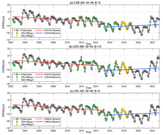
Figure 2.
Trends in EWH of land water in the North China Plain from GRACE/GRACE-FO SH inversions after SSA interpolation.
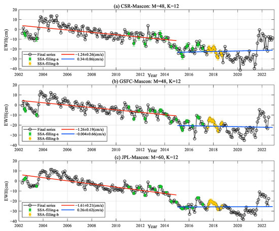
Figure 3.
Trends in EWH of land water in the North China Plain from GRACE/GRACE-FO Mascon inversions after SSA interpolation.
For the EWH variation time series obtained from the inversion of the above six products, the trend values were calculated using the Sen’s slope estimator and the Mann–Kendall trend test [26] was performed. The null hypothesis for the test was that there was no monotonic trend in the series, and the results are listed in Table 2. p is the confidence level, which is used to measure the probability that the null hypothesis holds, slope equals the Theil–Sen estimator/slope, z is normalized test statistics, and Tau is the Kendall Tau.
Table 2.
Six products’ EWH change time series trend values and trend test results.
The results of the above time series tests all have a p value of 0.00, which is less than the significance level (alpha = 0.05), and the null hypothesis is rejected, i.e., the time series was considered to have the significant trend.
In addition, the Pettitt test [27] was used to determine change points and the significance level of detected change points and the results are presented in Figure 4.
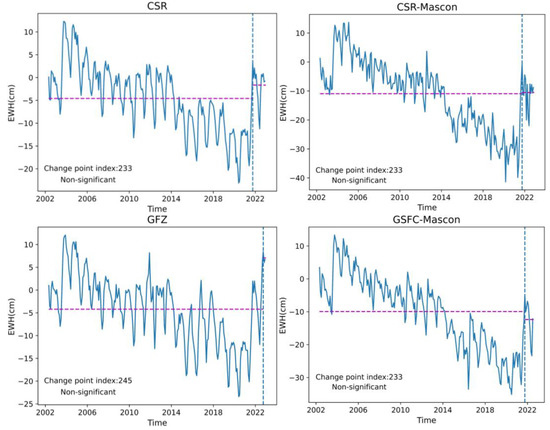
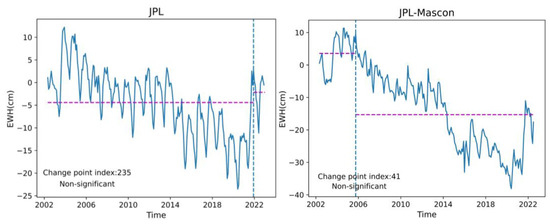
Figure 4.
Six products’ EWH time series Pettitt test for the change point and significance level of the detected point.
The results show that none of the six product change points were significant, concluding that sudden changes in the TWS of the North China Plain were not significant. The trends of each grid point in the North China Plain from 2002 to 2014 and 2015 to 2022 were calculated separately to obtain the spatial and temporal distribution of the trends in TWS, as presented in Figure 5 and Figure 6.
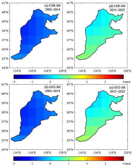
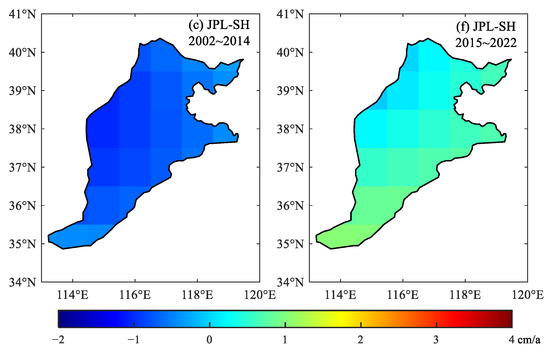
Figure 5.
April 2002~December 2014, spatial–temporal distribution of TWS in the North China Plain based on (a) CSR-SH, (b) GFZ-SH, and (c) JPL-SH inversion; January 2015~December 2022, spatial–temporal distribution of TWS in the North China Plain based on (d) CSR-SH, (e) GFZ-SH, and (f) JPL-SH inversion.
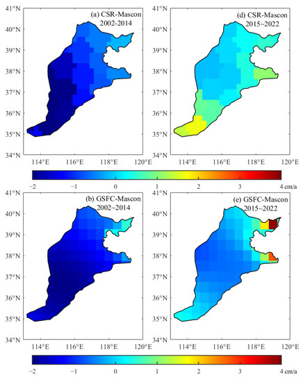
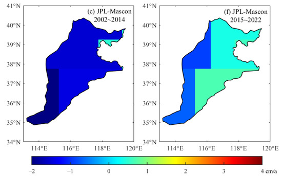
Figure 6.
April 2002~December 2014, spatial–temporal distribution of TWS in the North China Plain based on (a) CSR-Mascon, (b) GSFC-Mascon, and (c) JPL-Mascon inversion; January 2015~December 2022, spatial–temporal distribution of TWS in the North China Plain based on (d) CSR-Mascon (e) GSFC-Mascon, and (f) JPL-Mascon inversion.
The results reveal a sustained long-term trend in water storage deficit in the North China Plain. Water resources are scarce in the region because of its dense population, and residents primarily rely on utilizing groundwater as a source of water; thus, the water reserves in the North China Plain showed a gradual loss from 2002 to 2014. However, the inversion of the terrestrial water reserves of the plain based on the SH coefficients and Mascon solutions from 2002 to 2004 both showed an increasing trend; by looking up the precipitation data of the region, we found that the North China Plain experienced favorable water conditions in 2003, characterized by reduced groundwater extraction, aligning with the aforementioned trend. In terms of spatial distribution, Beijing and Tianjin exhibited more severe water deficits. The Beijing–Tianjin–Hebei region, as a significant industrial and agricultural hub in China with a high population and substantial water demand, experienced relatively intense groundwater exploitation. Moreover, the convergence zone between the North China Plain and the Taihang Mountains displayed a reduced rate of water storage deficit due to the obstruction and uplift of the southeast monsoon being on the eastern slopes of the Taihang Mountains, leading to topographic rainfall and more abundant precipitation.
By comparing the spatial and temporal distribution of water storage changes on land in the North China Plain between the two time periods, it can be found that in the plain, the rate of water storage loss has significantly decreased since the South-to-North Water Transfer Project began distributing water in 2015. The continuous annual increment in water supply from the project has resulted in a slight recovery of water storage in the North China Plain. In 2021, there was a significant upward trend in water storage changes in the plain, consistent with the long duration and high rainfall of the heavy precipitation process in the flood season of the region in that year. From the spatial recovery pattern, the rising trend in water storage in the northern part of the plain, mainly in Beijing and Tianjin, is more significant. Whereas there are large differences in the spatio-temporal distribution based on the spherical harmonic coefficients and Mascon inversions, differences in processing strategies may account for the discrepancies between the two categories mentioned above.
The results of the 2002–2014 equivalent water height trends and water storage change rates based on the inversions of the six models above are shown in Table 3, and the 2015–2022 equivalent water height trends and water storage change rates are shown in Table 4. Since the strong precipitation process in the 2021 flood season greatly accelerates the rising trend in water reserve in the North China Plain, which is inconsistent with the slow rising trend shown in previous years by the influence of water supply from the South-to-North Water Transfer Project, the uncertainty in the trend in EWH and water storage in Table 4 is greater.
Table 3.
High variation trend in equivalent water and change rate of water reserves from 2002 to 2014.
Table 4.
High variation trend in equivalent water and change rate of water reserves from 2015 to 2022.
The results indicate that the difference between the above six types of water storage trends based on gravity satellite observations before and after the South-to-North Water Transfer are 13.92 Gt/a, 13.40 Gt/a, 13.76 Gt/a, 16.96 Gt/a, 13.48 Gt/a, and 20.01 Gt/a, respectively. The annual rates of water storage change derived from the three types of SH coefficient products CSR-SH, GFZ-SH, and JPL-SH inversions demonstrate better alignment with the average annual water transfer of the project. The results obtained from the GSFC-Mascon inversion are better than those from CSR-Mascon and JPL-Mascon. The large difference in the agreement between the SH coefficient solution and Mascon solution inversion results and the annual average water delivery of the South-to-North Water Transfer is mainly due to the different data processing methods. The differences between the three types of SH solutions are small and the differences between the three types of Mascon solutions are large, mainly due to the fact that the SH solutions are all calculated using the traditional kinetic integration method, whereas the Mascon solutions are calculated using the regularization method, although they all use the regularization method, but there are differences in the form of establishing the observation equations and inconsistencies in the form of the regularization matrix, resulting in large differences in the Mascon solutions.
The CSR-SH data with the best fit were selected to assess the results, which show that the South-to-North Water Transfer Project has a significant mitigating effect on the declining trend in water storage in the plain, which has continued to rebound in recent years from −8.48 Gt/a to 5.44 Gt/a. To examine the validity of the present results, we compared them with studies carried out by previous authors. Su et al. [28] inverted TWS in North China from 2002 to 2010 with a rate of change of −1.1 cm/a. Moiwo et al. [29] estimated the change in TWS in the North China Plain between 2002 and 2009 with a deficit rate of −1.68 cm/a. Compared to these results, the results obtained based on Mascon are more reasonable, whereas those based on SH are slightly smaller. However, given the different lengths of data used in the study and the noise error at the edge of the region using a multi-scale gain factor, these results generally show a more consistent trend. The differences between the results are mainly due to the following reasons: (1) The length of the time period used for the observations and the delineation of the study area differ from those of previous authors. The relatively long time period of the observations selected in this study is more conducive to the overall study of the changes before and after the water transfer project. (2) We filled in the missing data in GRACE through SSA interpolation, which is more consistent with the real water storage trends than the original time series with missing data. (3) The multi-scale gain factor method is dependent on the hydrological model used, and the application of hydrological models in the North China Plain is not without some degree of ambiguity.
3.2. Comparison Based on Measured Well Data
The separation of groundwater from terrestrial water based on the water mass balance equation requires deduction of the contributions of canopy water and snow water in addition to soil water storage. The seasonal magnitude of gravitational variation due to biomass change is up to 5 mm, but is still an order of magnitude smaller than the GRACE/GRACE-FO uncertainty (2 cm) and therefore the change in canopy water is negligible [30]. In addition, the change in snow water relative to terrestrial water is also calculated to be negligible. Then, the change in groundwater storage based on GRACE/GRACE-FO can be equal to the change in total TWS minus soil water’s change.
We select RMSE and NSE as quantitative indicators to assess the consistency between the changes in groundwater storage based on GRACE/GRACE-FO and the changes in water storage in measured wells, and select the measured well data as the reference series to draw the Taylor diagram [31] to compare the accuracy of different models, so as to compare and analyze the inversion effects of six types of GRACE/GRACE-FO products in the North China Plain. The consistency results are presented in Table 5 and Figure 7 shows the Taylor diagram for the different models.
Table 5.
Quantitative index of consistency between groundwater reserve changes and measured well water reserve changes based on GRACE/GRACE-FO.
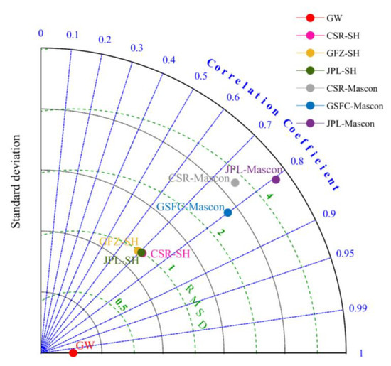
Figure 7.
Taylor diagram of six time-varying gravity field models.
The results demonstrate that all six categories exhibit NSE values exceeding 0.5 and small RMSE values, indicating a high agreement with the measured well water storage variability. In the Taylor diagram, the SD, RMSD and correlation coefficients of SH products are smaller than those of Mascon products, with the CSR-SH having the smallest SD and RMSD values and the correlation coefficient of about 0.7. Therefore, it is concluded that the CSR-SH-based groundwater storage variation exhibits the highest agreement with the measured well data and achieves the most effective inversion, while the JPL-Mascon-based inversion demonstrates lower effectiveness.
Figure 8a shows the time series of TWS changes in the North China Plain from 2005 to 2018 in the CSR-SH inversion. The equivalent water height decreased at (−0.76 ± 0.08) cm/a and the TWS decreased at (−9.68 ± 1.06) Gt/a during the whole study period. Figure 8b presents the time series of soil water storage changes in the plain based on the GLDAS_Noah model, where there is an annual variation in soil water storage changes in the region, with the equivalent water height changing at (−0.11 ± 0.10) cm/a and the decreasing trend in soil water storage at (−1.40 ± 1.25) Gt/a during the research phase. The time series of groundwater storage in the plain obtained after deducting soil water from land water is depicted in Figure 8c, where the equivalent water height of groundwater in the North China Plain based on CSR-SH inversion decreased at (−0.66 ± 0.08) cm/a from 2005 to 2018, and the groundwater storage decreased at (−8.28 ± 1.04) Gt/a; the time series of groundwater storage changes based on measured well data is presented in Figure 8d. The measured groundwater level in the North China Plain declined at a rate of (−0.22 ± 0.02) m/a during the research phase, and was multiplied by Fei’s [32] proposed feedwater degree of 0.03 to obtain the equivalent water height declining at a rate of (−0.65 ± 0.06) cm/a and groundwater storage declining at a trend of (−8.24 ± 0.08) Gt/a, which is in good agreement with the trend of (−8.28 ± 1.04) Gt/a obtained from the CSR-SH inversion.
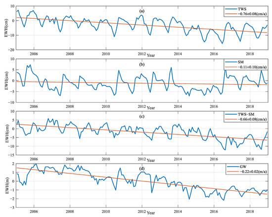
Figure 8.
January 2005~December 2018, (a) Time series of TWS in the North China Plain based on CSR-SH inversion; (b) Fitting trend in time series of soil moisture storage changes; (c) Time series of groundwater reserves change obtained by TWS−SM; (d) Fitting trend in measured groundwater table change time series.
The trend values of the above time series are calculated using the Sen’s slope estimator, followed by the Mann–Kendall trend test and Table 6 shows the results.
Table 6.
TWS, SM, TWS-SM and GW time series Mann–Kendall trend test results.
The p values for the TWS, SM, TWS-SM, and GW time series test results were all 0, less than the significance level (alpha = 0.05), indicating a significant trend in the TWS, SM, TWS-SM, and GW time series. The Pettitt test was used to determine points of change and the level of significance of the change points and results are shown in Figure 9.
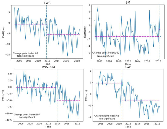
Figure 9.
TWS, SM, TWS−SM, and GW time series Pettitt test for the change points and significance level of the detected points.
The results show that all change points were nonsignificant, concluding that the abrupt changes in terrestrial, soil, and groundwater storage in the North China Plain were insignificant.
3.3. Influence of Meteorological Factors on Changes in Water Reserves in the North China Plain
To further assess the causes of TWS variability in the North China Plain, this section discusses the influence of meteorological factors on TWS variability in the plain. We used the precipitation, evaporation, and runoff data given by GLDAS_Noah [33] to calculate the TWS in the plain as a means of determining the influence of meteorological factors on the total TWS. Using the water balance equation:
where P, R, and E denote month-by-month precipitation, runoff, and evaporation, respectively. For each of these meteorological factors, their cumulative amounts were calculated separately, and their rates of change over the two periods were calculated by fitting the trends in segments using 2015 as the node. The results are listed in Table 7.
Table 7.
Comparison between the change rate of water reserves in the North China Plain and the average amount of water transferred through the South-to-North Water Transfer Project. Gt/a.
The rates of change in TWS during the two time periods were −0.10 Gt/a and −0.07 Gt/a, respectively, indicating a negative contribution of meteorological factors to TWS. The negative trend from 2015 to 2022showed a deceleration compared to the period of 2002–2014, thereby partially alleviating the water storage deficit in the North China Plain. However, compared to the South-to-North Water Transfer rate (13.91 Gt/a), the mitigating trend in water storage deficit due to meteorological factors (0.03 Gt/a) can only explain a small part of the post-2015 variation in the total water storage rate and is not a major factor.
Before the implementation of the South-to-North Water Transfer Project, the rate of water storage loss observed with GRACE/GRACE-FO was much higher than that caused by meteorological factors, suggesting that anthropogenic depletion of water resources in the North China Plain is the main factor in water storage loss. The rate of loss of TWS based on meteorological data remained unchanged after the commissioning of the middle and east lines of the project, whereas the rate of change in total water storage observed with GRACE/GRACE-FO increased by nearly two-fold, indicating that the project has significantly reduced the water deficit in the plain.
The significant disparity between TWS obtained from meteorological data and GRACE/GRACE-FO results is due to the large uncertainty in the runoff data of the GLDAS hydrological model, which does not take into account the influence of human activities such as the large-scale groundwater abstraction for agricultural irrigation in Northern China. In addition, the difference between them at the time before and after the project is indicative of the influence of meteorological factors on water storage.
3.4. Comparing Residuals Based on Time Series Decomposition
Multiple linear regression was used to decompose the time series of terrestrial water storage in the inversion of the six types of models, and the obtained results of the model residuals are listed in Table 8 below.
Table 8.
Residuals from time series decomposition of TWS changes from GRACE/GRACE-FO inversions. (cm).
It could be found that among the SH products, the time series of TWS changes based on CSR-SH and JPL-SH inversions had the smallest residuals in the North China Plain; among the Mascon products, the time series of TWS changes based on GSFC-Mascon inversions had the smallest residuals in the area. The difference between the residuals obtained with CSR-SH and JPL-SH was minimal, due to the similarity in data processing methods between the two agencies.
3.5. Estimating Uncertainty Based on the TCH Method
In order to comparatively study the noise variance of TWS changes in the North China Plain from GRACE/GRACE-FO product inversions, we used the TCH method to estimate the uncertainty in the time series of terrestrial water storage for six types of model inversions. The results are as shown in Table 9 below, where std is the zero-mean white noise process (representing the measurement error), here denoting the noise deviation of the corresponding GRACE/GRACE-FO processing center [34]. Additionally, xd_std is the relative value of std to the original time series.
Table 9.
Uncertainty of time series of TWS changes in GRACE/GRACE-FO inversions.
It can be found that the uncertainty of the time series of TWS changes based on GSFC-Mascon inversion was the smallest in the North China Plain, whereas the uncertainty of JPL-Mascon was the largest, and the overall noise variance of all six types of GRACE/GRACE-FO products was small. Then, we used the TCH method to estimate the uncertainty distribution of TWS changes in the plain for the inversion of the above six types of GRACE/GRACE-FO raw grid data, as presented in Figure 10.
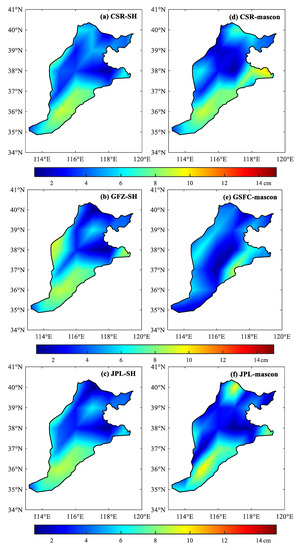
Figure 10.
The uncertainty of water reserve changes in the North China Plain calculated with GRACE/GRACE-FO.
Overall, the spatial distribution of uncertainty in TWS changes across the North China Plain is in line with the uncertainty results from the time series calculations above, with GSFC-Mascon having less uncertainty than the other models and GFZ-SH and JPL-Mascon having higher uncertainty. In the southern region of the plain, the uncertainty of the GRACE/GRACE-FO inversion is large. Additionally, in the border areas of the plain, there are large spatial differences in water storage variability. The uncertainty based on CSR-SH is in high agreement with that based on JPL-SH inversions. Considering that the two time-varying gravity field models and the methods used are relatively similar, the results are laterally justified.
3.6. Comprehensive Factor Evaluation of Inversion Effect
Combining the above various types of methods, the results of the comprehensive evaluation of the inversion effect are shown in Table 10.
Table 10.
Results of the comprehensive evaluation of inversion effects from good to bad.
From a practical standpoint, the inversion results based on various SH coefficients and Mascon solutions are more consistent with the actual situation of the products with good consistency with the water supply and well data of the project, and the products are recognized as having better quality. Combining the two methods of time series decomposition and TCH, the analysis concludes that among the SH products, CSR-SH and JPL-SH have better inversions, and the differences in uncertainties obtained are minimal due to the similar data processing strategies of the two organizations; among the Mascon solutions, GSFC-Mascon has the best inversions. The uncertainties calculated using the time series decomposition and TCH methods both overestimate or underestimate the true uncertainties, and only reflect the internal conformity accuracy of the inversion of the equivalent water height variation time series of the North China Plain based on various types of time-varying gravity fields, and have less impact on the assessment of whether the inversion effect conforms to the actual situation. Therefore, this study concludes that based on the influence of South-to-North Water Transfer on variations in water reserve in the North China Plain, CSR-SH is the best inversion.
4. Discussion
4.1. Analysis of the Inconsistency between the Results of the TCH Calculation and the Rest of the Methods
Considering the obvious differences in the ranking of the uncertainty results for the six types of time-varying gravity fields calculated using the TCH and the ranking of the consistency results between the inverse EWH time series and the water supply from the South-to-North Water Transfer Project, the measured well data, and the ranking of the magnitude of the residuals obtained from the time series decomposition, this section further analyses the reasons for the inconsistency between the results of the TCH method and the rest of the various methods.
The product with the lowest uncertainty obtained with TCH calculations was GSFC-Mascon. The latest version of the GSFC-Mascon products applies the latest background uptake dynamics model and L1B data. Months of GRACE-FO uses the new ACH0 accelerometer transplant file (solutions after April 2022). According to Loomis et al. [10], the GSFC-Mascon products improve the strength of signal recovery and reduce noise relative to the monthly SH and other Mascon products. Therefore, we consider the results calculated with the TCH method to be somewhat reasonable.
In a physical sense, the existence of external reference data was analyzed by comparing the inverse EWH time series with the water supply of the project and the measured well data, which is an external conformity accuracy check. The time series decomposition, on the other hand, is a multiple linear regression analysis to check the temporal variability of TWS, reflecting the signal strength of a single time-varying gravity field inversion time series of EWH variation in the North China Plain. The TCH method, on the other hand, is used to calculate std as a zero-mean white noise process, indicating the noise deviation of the corresponding product, an internal conformity accuracy check. The signal common to each series is removed by forming pairs of differences between the time series, so that the assumed value of the true signal is not required. When appropriate assumptions are made regarding the correlation between the series, the uncertainty of each series can be retrieved from the variance of the difference series [35]. The TCH method is used to estimate the relative uncertainty of six types of inverse time series in the absence of a reference dataset, reflecting the in-conformity accuracy between the six types of time-varying gravity field inverse time series. As the uncertainties calculated with both the time series decomposition and TCH methods overestimate or underestimate the true uncertainties, there is also a lack of external data as a reference for comparison, and it may be more accurate to use external checks of water wells or South-to-North Water Transfer volumes for the assessment results of the inversion effects of the six categories of products. In addition, previous studies such as Li [4], Zhang [5] and He [6] have used CSR-SH products for inversion, which also confirms that the CSR-SH model works best for inversion in the North China Plain.
4.2. Explanation for the Differences between SH Coefficient and Mascon Products
From the results in Section 3.1, it can be seen that there is a large discrepancy between the results inverted from the SH coefficient products and Mascon products. Therefore, the reasons for such differences are further analyzed and discussed in this section.
The most important feature of Mascon products compared to the traditional SH coefficients is that no smoothing filtering postprocessing is required. Traditional spherical harmonics require postprocessing such as low-order term replacement and supplementation, strip removal, GIA correction, etc. before they can be restored to their gridded EWH. While the Mascon products provide the gridded products directly, the postprocessing process, including GIA correction, is carried out before release and can be used directly. The SH coefficient products use the traditional kinetic integration method to establish interstellar observations as a function of SH coefficients during data processing, whereas the Mascon products directly establish Level 1B data as a function of the EWH of the grid, using a regularization method to deal with north–south strip noise. In addition, another feature of the Mascon products is that leakage errors are taken into account. Because of the spatial observations of the GRACE satellites and the removal of striping errors, the gravity signal recovered with GRACE can leak from the mass source region where it was generated to other regions, such as land signals to the ocean, seismic signals to the ocean, etc. The Mascon products, however, take into account and partially recover the leakage errors. For the SH coefficient products, a multi-scale factorization method was used to recover the leakage error. The multi-scale factor method, however, relies on the hydrological model used, and there is some uncertainty in using the hydrological model in the North China Plain. Therefore, this paper recognizes that the above is the main reason for the large discrepancy between the results of the Mascon products inversion and the SH coefficient products.
In addition, there are large differences in the inversion results between Mascon products, due to different data processing strategies. CSR-Mascon products use the SH coefficient as a transition to establish the observational equations when establishing the interstellar observations as a function of the EWH of the grid. JPL-Mascon products use exact partial differential equations to establish the functional expressions for the spacing data and the Mascon solutions when recovering the Mascon solutions. GSFC-Mascon products, on the other hand, are based on star spacing velocities or star spacing accelerations, and unlike JPL-Mascon, each Mascon basis function is not expressed analytically, but as a truncated finite order expression of the spherical harmonic coefficients [36]. Although the Mascon solutions are calculated using the regularization method, there are differences in the form of the established observation equations, inconsistencies in the regularization parameters and in the construction of the regularization matrix, the design of which directly affects the accuracy of the inverse Mascon solutions. If it is over-constrained, it can result in a weakening of the signal peak, and under-constraining it can result in a large number of strip errors filling the entire Mascon solution. As a result, there is a large variation between the inversion results of different Mascon products.
5. Conclusions
In this study, we calculated the changes in TWS in the North China Plain, respectively, by using GRACE/GRACE-FO products, including CSR-SH, GFZ-SH, JPL-SH, CSR-Mascon, GFSC-Mascon, and JPL-Mascon. These changes were compared with the water supply data of the South-to-North Water Transfer Project to assess the effects of the project on the terrestrial water, soil water, and groundwater storage in the plain. By comparing with the water supply data of the project and measured well data, and using the TCH method to calculate the uncertainty, we analyzed the inversion effect of the above six kinds of time-varying gravity field models. The results show that the middle and east lines of the project have greatly alleviated the loss of TWS in the plain since the end of 2014, from −8.48 Gt/a to 5.44 Gt/a, indicating that the project has a positive effect on the water supply in the area. It also contributes to the gradual recovery of groundwater in the North China Plain after long-term overexploitation. This study serves as a valuable reference for China’s water resource management decisions.
From practical considerations, by comparing the consistency of the inversion results of the six time-varying gravity field models (CSR-SH, GFZ-SH, JPL-SH, CSR-Mascon, GSFC-Mascon, and JPL-Mascon) with the water supply of the South–North Water Transfer Project and the measured groundwater well data, as well as the uncertainties derived from TCH, it was concluded that CSR-SH is the best inversion based on the impact of the project on water storage changes in the North China Plain. This study integrated and compared the inversion effects of various types of SH with Mascon products, which is indicative for the selection of time-varying gravity fields in subsequent studies.
Furthermore, certain quality changes outside the study area may have infiltrated the study area during the data processing phase, resulting in errors in the calculation results of the study area [4]. With the accumulation of GRACE Follow-On data and their further evaluation and optimization, we believe that the variation trend in water reserves in the North China Plain will be more accurately estimated, and then the mitigation effect of the South-to-North Water Transfer Project on the loss of water reserves and the inversion effect of various time-varying gravity fields in the North China Plain will be more accurately evaluated.
Author Contributions
Methodology, C.Z.; data curation, C.Z.; writing—original draft preparation, C.Z.; writing—review and editing, C.Z.; visualization, W.L. and C.Z.; supervision, W.L.; project administration, W.L. All authors have read and agreed to the published version of the manuscript.
Funding
This research received no external funding.
Institutional Review Board Statement
Not applicable.
Informed Consent Statement
Not applicable.
Data Availability Statement
The data presented in this study are available on request from the corresponding author.
Acknowledgments
The authors would like to thank Wei You and Xiangyu Wan of Southwest Jiaotong University for their guidance on this study and the reviewers for their comments.
Conflicts of Interest
The authors declare no conflict of interest.
References
- Zhang, Z.; Luo, G.; Wang, Z.; Liu, C.; Li, Y.; Jiang, X. Study on Sustainable Utilization of Groundwater in North China Plain. Resour. Sci. 2009, 31, 355–360. [Google Scholar]
- Feng, W.; Zhong, M.; Lemoine, J.; Biancale, R.; Hsu, H.-T.; Xia, J. Evaluation of groundwater depletion in North China using the Gravity Recovery and Climate Experiment (GRACE) data and ground-based measurements. Water Resour. Res. 2013, 49, 2110–2118. [Google Scholar] [CrossRef]
- Zhao, Q.; Zhang, B.; Yao, Y.; Wu, W.; Meng, G.; Chen, Q. Geodetic and hydrological measurements reveal the recent acceleration of groundwater depletion in North China Plain. J. Hydrol. 2019, 575, 1065–1072. [Google Scholar] [CrossRef]
- Li, J.; Tang, H.; Rao, W.; Zhang, L.; Sun, W. Influence of South-to-North Water Transfer Project on the changes of terrestrial water storage in North China Plain. J. Univ. Chin. Acad. Sci. 2020, 376, 775–783. [Google Scholar]
- Zhang, M.; Wei, C. Analysis of the spatial and temporal variation of groundwater storage in the North China Plain based on multi-source data. J. Geod. Geodyn. 2022, 42, 5. [Google Scholar]
- He, G. Detecting water storage changes in the North China Plain based on GRACE RL06 data. Geospat. Inf. 2022, 006, 020. [Google Scholar]
- Swenson, S.; Chambers, D.; Wahr, J. Estimating geocenter variations from a combination of GRACE and ocean model output. J. Geophys. Res. Solid Earth 2008, 113, 410–421. [Google Scholar] [CrossRef]
- Cheng, M.; Tapley, B. Variations in the Earth’s oblateness during the past 28 years. J. Geophys. Res. Solid Earth 2004, 109, 402–410. [Google Scholar] [CrossRef]
- Save, H.; Bettadpur, S.; Tapley, B.D. High resolution CSR GRACE RL05 mascons. J. Geophys. Res. Solid Earth 2016, 121, 7547–7549. [Google Scholar] [CrossRef]
- Loomis, B.D.; Felikson, D.; Sabaka, T.J.; Medley, B. High-Spatial-Resolution Mass Rates From GRACE and GRACE-FO: Global and Ice Sheet Analyses. J. Geophys. Res. Solid Earth 2021, 126, e2021JB023024. [Google Scholar] [CrossRef]
- Wiese, D.N.; Yuan, D.-N.; Boening, C.; Landerer, F.W.; Watkins, M. JPL GRACE Mascon Ocean, Ice, and Hydrology Equivalent Water Height Release 06 Coastal Resolution Improvement (CRI) Filtered Version 1.0. Ver. 1.0. PO.DAAC; Jet Propulsion Laboratory: Pasadena, CA, USA, 2018. [Google Scholar] [CrossRef]
- Ek, M.; Mitchell, K.; Lin, Y.; Rogers, E.; Grunmann, P.; Koren, V.; Gayno, G.; Tarpley, J.D. Implementation of Noah land surface model advances in the National Centers for Environmental Prediction operational mesoscale Eta model. Geophys. Res. 2003, 108, 8851. [Google Scholar] [CrossRef]
- National Earth System Science Data Center. National Science & Technology Infrastructure of China. Available online: http://www.geodata.cn (accessed on 14 April 2023).
- Wahr, J.; Molenaar, M.; Bryan, F. Time variability of the Earth’s gravity field: Hydrological and oceanic effects and their possible detection using GRACE. J. Geophys. Res. Solid Earth 1998, 103, 30205–30230. [Google Scholar] [CrossRef]
- Farrell, W. Deformation of the Earth by Surface Loads. Rev. Geophys. 1972, 10, 761. [Google Scholar] [CrossRef]
- Yi, S.; Sneeuw, N. Filling the data gaps within GRACE missions using Singular Spectrum Analysis. J. Geophys. Res. Solid Earth 2021, 126, e2020JB021227. [Google Scholar] [CrossRef]
- Swenson, S.; Wahr, J. Methods for inferring regional surface-mass anomalies from Gravity Recovery and Climate Experiment (GRACE) measurements of time-variable gravity. J. Geophys. Res. Solid Earth 2002, 107, 2193–2205. [Google Scholar] [CrossRef]
- Klees, R.; Zapreeva, E.; Winsemius, H.; Savenije, H.H.G. The bias in GRACE estimates of continental water storage. Hydrol. Earth Syst. Sci. 2007, 11, 1227–1241. [Google Scholar] [CrossRef]
- Landerer, F.; Swenson, S. Accuracy of scaled GRACE terrestrial water storage estimates. Water Resour. Res. 2012, 48, 531–541. [Google Scholar] [CrossRef]
- Yang, P.; Xia, J.; Zhan, C.; Qiao, Y.; Wang, Y. Monitoring the spatio-temporal changes of terrestrial water storage using GRACE data in the Tarim River basin between 2002 and 2015. Sci. Total Environ. 2017, 595, 218–228. [Google Scholar] [CrossRef]
- Feng, W. GRAMAT: A comprehensive Matlab toolbox for estimating global mass variations from GRACE satellite data. Earth Sci. Inform. 2019, 12, 389–404. [Google Scholar] [CrossRef]
- Moriasi, D.; Arnold, J.; Liew, M.; Bingner, R.; Harmmel, R.; Veith, T. Model evaluation guidelines for systematic quantification of accuracy in watershed simulations. Trans. ASABE 2007, 50, 885–900. [Google Scholar] [CrossRef]
- Koot, L.; De, V.; Dehant, V. Atmospheric angular momentum time-series: Characterization of their internal noise and creation of a combined series. J. Geod. 2006, 79, 663–674. [Google Scholar] [CrossRef]
- Galindo, F.; Palacio, J. Post-processing ROA data clocks for optimal stability in the ensemble timescale. Metrologia 2003, 40, S237–S244. [Google Scholar] [CrossRef]
- Galindo, F.; Palacio, J. Estimating the instabilities of N correlated clocks. In Proceedings of the 31th Annual Precise Time and Time Interval Systems and Applications Meeting, Real Instituto y Observatorio de la Armada, Dana Point, CA, USA, 7–9 December 1999; pp. 285–296. [Google Scholar]
- Fatichi, S. Mann-Kendall Test, MATLAB Central File Exchange. 2023. Available online: https://www.mathworks.com/matlabcentral/fileexchange/25531-mann-kendall-test (accessed on 6 June 2023).
- Dey, P. Pettitt Change Point Test for Univariate Time Series Data, MATLAB Central File Exchange. 2023. Available online: https://www.mathworks.com/matlabcentral/fileexchange/60973-pettitt-change-point-test-for-univariate-time-series-data (accessed on 7 June 2023).
- Su, X.; Ping, J.; Ye, Q. Terrestrial water variations in the North China Plain revealed by the GRACE mission. Sci. China Earth Sci. 2011, 54, 1965–1970. [Google Scholar] [CrossRef]
- Moiwo, J.; Tao, F.; Lu, W. Analysis of satellite-based and in situ hydro-climatic data depicts water storage depletion in North China Region. Hydrol. Process. 2013, 27, 1011–1020. [Google Scholar] [CrossRef]
- Rodell, M.; Chao, B.; Au, A.; Kimball, J.S.; McDonald, K.C. Global biomass variation and its geodynamic effects. Earth Interact. 2005, 9, 1–19. [Google Scholar] [CrossRef]
- Taylor, K. Summarizing multiple aspects of model performance in a single diagram. J. Geophys. Res. Atmos. 2001, 106, 7183–7192. [Google Scholar] [CrossRef]
- Fei, Y.; Jian, M.; Zhang, Z.; Qian, Y.; Chen, J.; Li, Y. Application of General Specific Yield in North China Plain Groundwater Resources Assessment. South-to-North Water Transf. Water Sci. 2010, 8, 55–59. [Google Scholar]
- Rodell, M.; Houser, P.; Jambor, U.; Gottschalck, J.; Mitchell, K.; Meng, C.-J.; Arsenault, K.; Cosgrove, B.; Radakovich, J.; Bosilovich, M.; et al. The global land data assimilation system. Bull. Am. Meteorol. Soc. 2004, 85, 381–394. [Google Scholar] [CrossRef]
- Ferreira, V.; Montecino, C.; Henry, D.; Kelly, C.; Heck, B. Uncertainties of the Gravity Recovery and Climate Experiment time-variable gravity-field solutions based on three-cornered hat method. J. Appl. Remote Sens. 2016, 10, 015015. [Google Scholar] [CrossRef]
- Chin, T.; Gross, R.; Dickey, J. Multi-reference evaluation of uncertainty in earth orientation parameter measurements. J. Geod. 2005, 79, 24–32. [Google Scholar] [CrossRef]
- Zhang, L.; Sun, W. Progress and prospect of GRACE Mascon product and its application. Rev. Geophys. Planet. Phys. 2022, 53, 35–52. [Google Scholar] [CrossRef]
Disclaimer/Publisher’s Note: The statements, opinions and data contained in all publications are solely those of the individual author(s) and contributor(s) and not of MDPI and/or the editor(s). MDPI and/or the editor(s) disclaim responsibility for any injury to people or property resulting from any ideas, methods, instructions or products referred to in the content. |
© 2023 by the authors. Licensee MDPI, Basel, Switzerland. This article is an open access article distributed under the terms and conditions of the Creative Commons Attribution (CC BY) license (https://creativecommons.org/licenses/by/4.0/).