Application of Machine Learning for Prediction and Monitoring of Manganese Concentration in Soil and Surface Water

Abstract

This study explored the application of machine learning, specifically artificial neural network (ANN), to create prediction models for manganese (Mn) concentration in soil and surface water (SW) on the island province with two open mine pits overflowing to two major rivers that experienced mining disasters. The two ANN models were created to predict Mn concentrations in soil and SW from 12 and 14 input parameters for soil and SW, respectively. These input parameters were extracted from extensive field data collected at the site during sampling program in 2019, 2021, 2022, and initially processed with spatial analysis via geographic information system (GIS). All datasets were then divided for model training and validation, using 85% and 15% ratio, respectively. Performance evaluation of each model with mean absolute percentage error (MAPE) and root mean squared error (RMSE) confirmed the accuracy of both models. The soil Mn model achieved MAPE and RMSE values of 2.01% and 23.98, respectively. The SW Mn model was split into two models based on SW Mn values within the 0–1 mg/L range and >1 mg/L range. The SW Mn model for >1 mg/L performed better with MAPE and RMSE of 4.61% and 0.17, respectively. Feature reduction was also conducted to identify how the models will perform if some input parameters were excluded. Result showed sufficient accuracy can still be obtained with the removal of 4–5 input parameters. This study and these models highlight the benefit of ANN to the scientific community and government units, for predicting Mn concentration, of similar environmental conditions.

1. Introduction

Protection of the environment is a major part of the United Nation’s sustainable development goals (SDGs), particularly SDG 2, 3, 6, 11, 13, 14, and 15 [1]. These SDGs demonstrate the critical importance of the environment in maintaining sustainable life in each country. Soil [1] and surface water (SW) [2,3] are the two media that should be given the most focus as they have high exposure to the accumulation of pollutants, while being accessible to human and animal consumption via various avenues, particularly food production [4,5]. According to food and agriculture organizations of the United Nations, 40.8% of Earth’s total surface is croplands, grasslands, and bare soils [6], while 0.27% of its freshwater is found in lakes and rivers [7].

Effective monitoring is essential to prevent or mitigate contamination in the environment that can adversely impact human health and natural ecosystems [8]. Despite significant advancements in instrumentation, environmental monitoring remains highly challenging due to various political and economic factors [9]. Hence, developing a tool that can predict metal concentration, such as manganese (Mn), could be useful in both data collection and evaluation, as well as making strategic programs and prompt decision. For instance, less developed countries have limited capacity to provide expensive equipment and expertise for effective monitoring [10]. Instead of always needing complex instruments, artificial intelligence (AI) may be used as an accessible alternative to characterize and/or predict environmental data [11,12]. Artificial neural network (ANN), which relies mainly on training data to learn and improve prediction capability, is now one of the most popular AI techniques to develop prediction models for security [13], economics [14], aerospace [15], healthcare [16], seismic activity [17], and weather forecasting [18], to name a few. ANN is a machine learning tool that combines related parameters to estimate a target parameter [19].

The accumulation of metals in soil and SW is influenced by various parameters that could be easily measured on site, such as soil pH [20], flood level and curve number [21], physicochemical properties of SW (i.e., pH, temperature, electric conductivity (EC), and total dissolved solids (TDS)) [12], river morphology [22,23], and atmospheric precipitation [24]. An ANN model would be highly beneficial if it was first trained on the relationship between accessible parameters and the target parameter (e.g., pH/TDS to metal concentration) and then used to predict future target parameter values from input parameter values only, without the need of complex equipment. Previous studies developed prediction models for soil [25,26] and water [27,28,29]; however, this study considered the physicochemical properties of both media, that are frequently monitored, to provide scientific-based information in making prompt decisions. In 2018, Shi et al. [30] demonstrated the very important role of hydrodynamic conditions on metal transport in rivers, where it induces more dispersion compared to hydrostatic conditions. Climate change could generate more frequent flooding in rivers [31], which can contribute to the accumulation of metals in both soil and SW [32]. High runoff rates can carry metals to rivers, which, in turn, can transfer to soils via adsorption and desorption [33,34].

Marinduque is an island province in the Philippines where extensive mining activities used to exist. Unfortunately, two catastrophic mining disasters [35] occurred in 1993 and 1996. In 1993, toxic mine tailings spilled from the San Antonio pit into the adjacent Mogpog River, while in 1996, a drainage tunnel burst in the Tapian pit, spilling 1.6 million m³ of mine tailings into Boac River. The soil and SW in both Mogpog and Boac River are now highly contaminated with toxic metals [21,35,36,37], posing a great environmental concern in the surrounding areas. Furthermore, no remediation strategies have been developed, and the two mining pits still exist and are liable to flooding and overflow during extreme storm events [38]. It is evident from studies conducted in 1998 [39] and 2019 [35] that the concentration of metals has increased in soil and SW over time, particularly Mn.

Mn is a naturally occurring element in soils that is essential to plant growth and reproduction [40]; however, excessive Mn can trigger oxidative stress and disrupt photosynthesis [41] while also being very harmful to humans. The exposure of humans to toxic amounts of Mn can result in neurotoxicity [42] and damage to the central nervous system [43]. According to the United States Environmental Protection Agency (USEPA), humans are only allowed to consume 0.14 mg/kg-day of Mn to avoid toxicity [44]. Alarming levels of Mn have been found in some agricultural products on the island of Marinduque, such as rice [36,45], and products in aqueous environments, such as crustaceans and tilapia [46]. Limited environmental monitoring has been performed in the area, with communities mostly unaware of the excessive levels of Mn in nearby soils and SW. Most of the municipalities in Marinduque are classified as third-class, and according to the report of Department of Trade and Industry, the total revenue for Marinduque was only PHP 682,353,324 (USD 12,565,898) in 2022 [47]. This highlights the challenge for the island to continuously monitor the environment with complex equipment.

Hence, the main objective of this study is to develop an ANN model to predict Mn concentration in soil and SW within the Mogpog and Boac river areas in Marinduque, Philippines. The developed model will reduce the need for complex and expensive equipment to estimate and predict metal concentrations in soil and surface water. Moreover, it will address the challenges in implementing sampling and analysis activities in rural areas where access to appropriate laboratories is difficult. These model predictions could provide guidance to local communities and government units to design and implement efficient mitigation strategies. This study specifically aims to: (i) spatially analyze Mn concentration from collected soil and SW samples within the areas surrounding the rivers; (ii) identify input parameters that have the highest association with the target parameter Mn; and (iii) develop and train an ANN model for both soil and SW to predict Mn concentration. The developed models could provide information that will aid in making prompt decisions that would contribute to socio-economic development of the island.

2. Materials and Methods

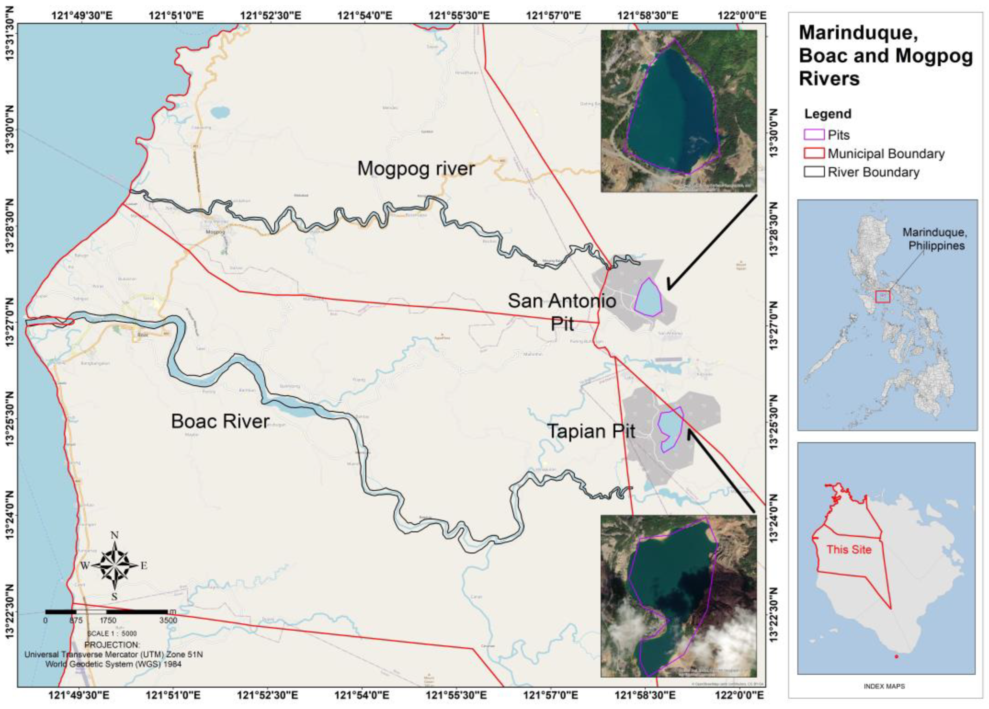
2.1. Project Site Location

Marinduque is an island province in the Philippines (Figure 1) that hosted extensive mining activities [48] using an open-mining pit process. Two of the worst mining disasters in the world occurred on the island in 1993 and 1996. Enormous volumes of toxic mine tailings spilled from the San Antonio and Tapian mine pits into the Mogpog and Boac Rivers, respectively [8], flooding neighboring towns and villages and heavily contaminating associated soil and surface water bodies. Although mining operations ceased after the disasters, the soil and SW within the rivers and surrounding areas remain contaminated [12,21,35,36,39]. Despite being abandoned, the two open pits produce sheet flows, especially during intense rainfall and flooding, that discharge mine tailings to both rivers and adjacent land [21]. This has resulted in significant increases in metal concentration from 1998 to 2019, particularly Mn, which increased from 1060 ppm to 68,169 ppm [35,39].

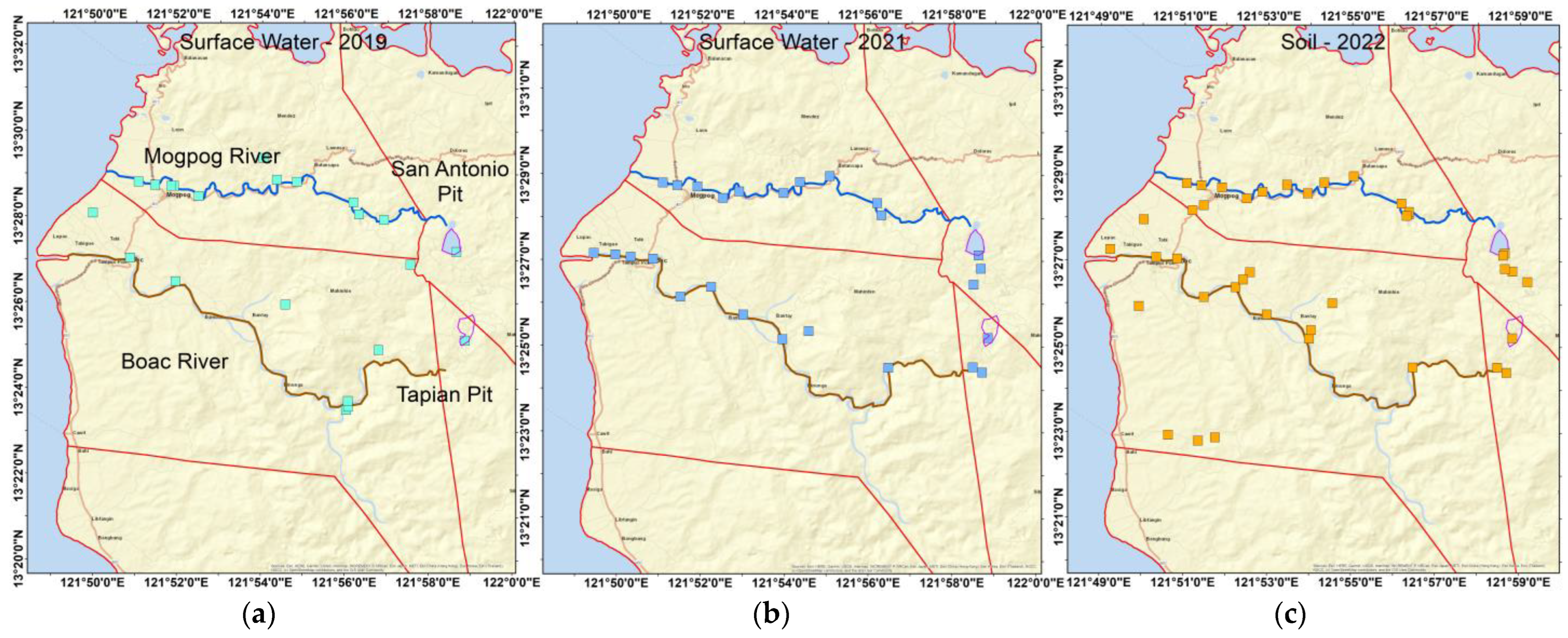
2.2. Soil and Surface Water Sampling in Mogpog and Boac Municipalities

Field sampling events were conducted in three different years to collect soil and SW samples in strategic locations inside the Mogpog and Boac municipalities only. The location of all sampling points is indicated in Figure 2, with most samples collected near the two rivers and the open mining pits. A total of 40 soil samples were collected in February 2022 by following the procedures outlined in the USEPA guidelines LSASDPROC-300-R4 [49], while 22 and 26 SW samples were collected in December 2019 and July 2021, respectively, using USEPA LSASDPROC-201 R5 [50].

The physicochemical properties of SW, such as pH, temperature, electric conductivity (EC), and total dissolved solids (TDS), were analyzed with a portable multi-parameter meter (HANNA, Woonsocket, RI, USA) with a HI1285-5 probe and accompanying calibration and cleaning solutions (e.g., HI70007, HI70031, HI70032, HI700661). The physicochemical properties of the soil, including pH, temperature, EC, and humidity, were also measured using a Renke portable soil analyzer with multi-probes. Soil moisture content (MC) was also calculated for the soil samples using the oven drying method. Mn concentrations in soil and SW were measured with a portable Olympus Vanta X-ray fluorescence (XRF) analyzer (Olympus, Bartlett, TN, USA) and Optima 8000 Inductively Coupled Plasma Optical Emission Spectrometry (ICP-OES) (PerkinElmer, Waltham, MA, USA), respectively. The ICP-OES used the multi-element standard solution IV and resulting R² equal to 0.99 during the analysis. The XRF was calibrated using its standard reference material and the Olympus Vanta blank in resealable plastic no. 2. The XRF device was extremely beneficial for measuring soil Mn as the study site is on a remote island without an appropriate analytical laboratory. It can analyze metal concentrations in soil samples, though the focus of this study is Mn, with a confidence level of 99.7% [51] and has been employed for a range of environmental monitoring studies [52,53,54].

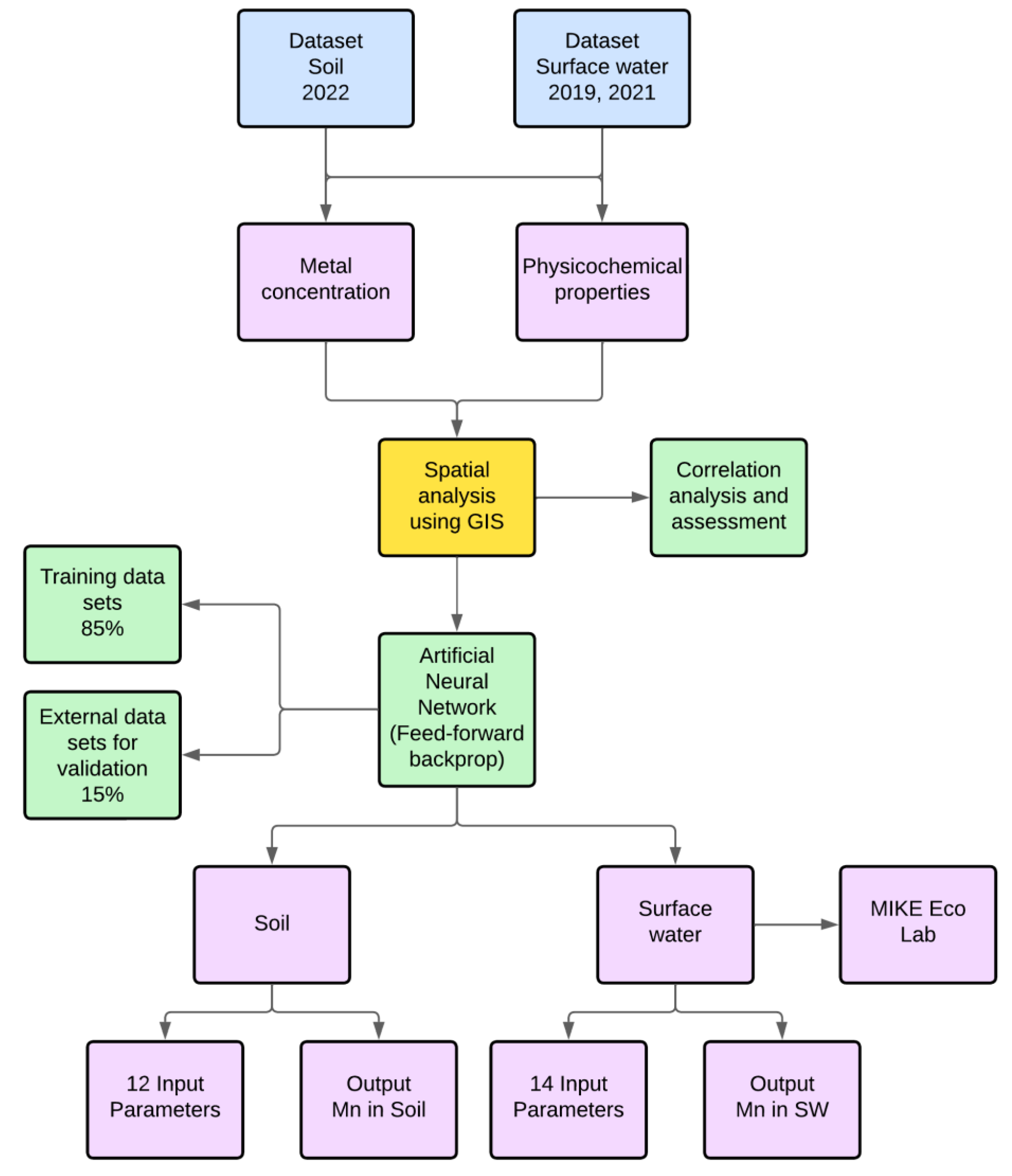
2.3. Prediction Model Development Framework

Figure 3 illustrates the framework that was developed to create the ANN prediction model aided by spatial analysis using a geographic information system (GIS). The two sets of data for SW (2019 and 2021) and the one set of data for soil (2022) contained the physicochemical properties and Mn concentrations measured at each sampling point. In this study, 12 parameters were considered in the prediction of soil Mn, namely pH, temperature, EC, humidity, soil MC, ground slope, ground elevation, curve number (CN), flood level, soil texture, average rainfall, and average atmospheric temperature. All these parameters were gathered using spatial analysis to assess their relationship to the corresponding Mn concentration in soil. Fourteen parameters were considered for SW, namely pH, temperature, EC/TDS, ground slope, ground elevation, CN, flood level, soil texture, average rainfall, average atmospheric temperature, and morphologic parameters such as river bends, river width, and sinuosity. Morphologic parameters for SW were employed to account for the hydrodynamics of the river.

Correlation analysis was also performed to determine the degree of relationship of the identified parameters in soil and SW to their respective concentration of Mn. Sets of spatial data were extracted with the aid of GIS, which were used to create the prediction model using ANN. For the training of the ANN model, 85% of all data extracted from the spatial analysis were used, with the remaining 15% used for external validation. External validation is very important to ensure that the trained model will perform strongly in predicting data outside of the datasets used for training [55]. MIKE Eco Lab was used to validate river morphology parameters as an additional input to the ANN model that significantly affects Mn accumulation in SW.

2.3.1. GIS Spatial Analysis of Identified Parameters

Spatial analysis was performed using a GIS to convert point data into spatially continuous data, with systematic interpolation assigning data to unsampled sites. Spatial interpolation is widely employed in environmental studies, where it can be highly effective [56] in improving the assessment of an area’s condition [57,58]. In this study, the inverse distance weighting (IDW) method was used to estimate values in unsampled locations using the weighted average of known data points, with these weights inversely correlated to the distances between the sampled and predicted points.

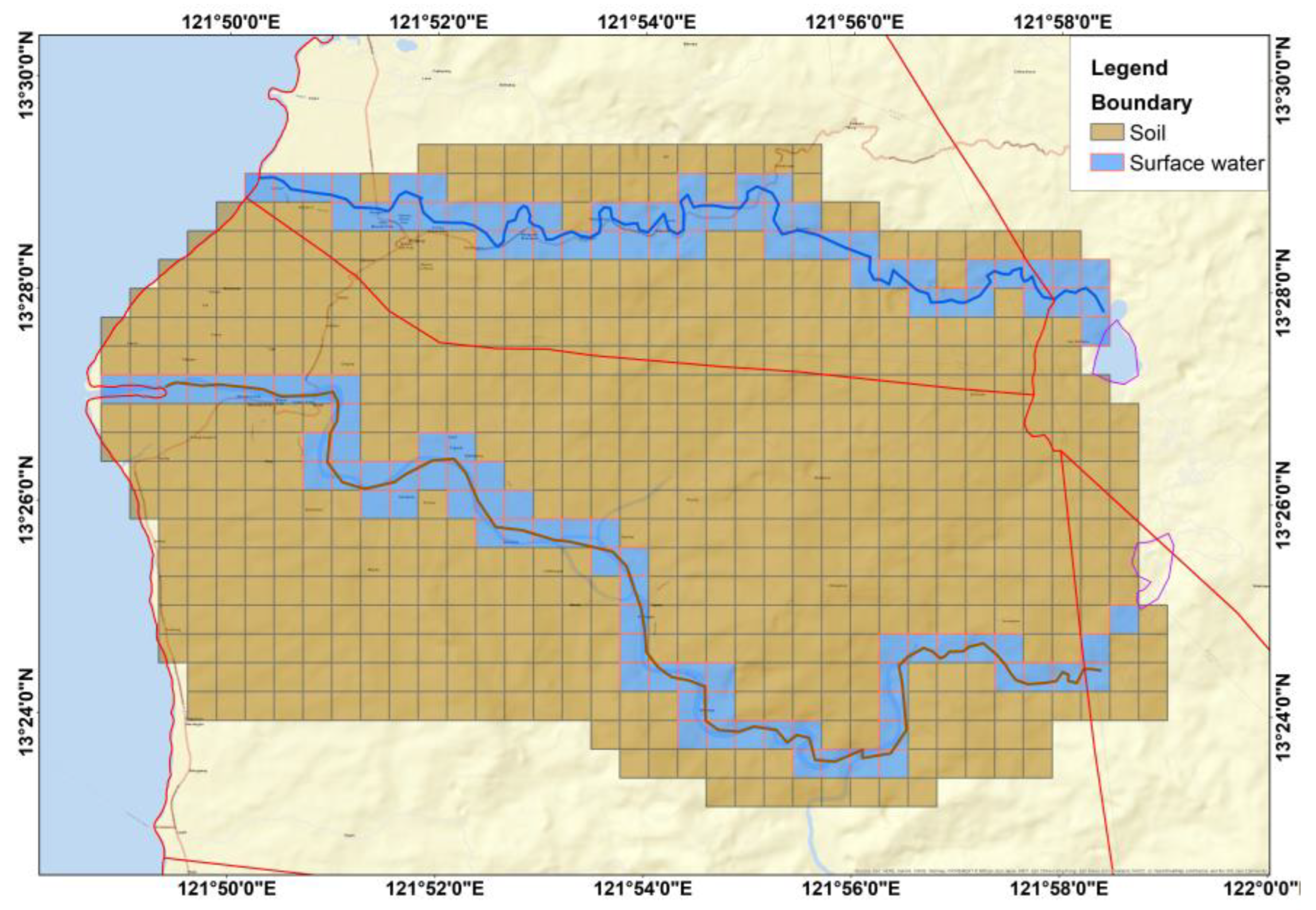
2.3.2. Spatial Grid Mapping and Zonal Statistics

Grid mapping was performed on the study area to assign spatial data to specific locations [59]. While point data only represent a value specific to that location, grid data take the average of all point data enclosed within each node using zonal statistics [60]. Figure 4 presents the developed grid map with a node size of 500 m, with soil and SW having 563 and 117 grid nodes, respectively. Note that both 2019 and 2021 SW data consisted of 117 grid nodes and were lumped together into a single SW dataset with 234 nodes.

The spatial grid nodes and zonal statistics were integrated to assign and process data for each identified input parameter. A variety of maps were superimposed over the gridded map to determine the various parameters: (i) CN was determined from land cover maps; (ii) ground elevation, ground slope, and river morphology were determined from digital elevation models such as in-SAR; (iii) flood level from hazard maps of the Mines and Geosciences Bureau; (iv) soil texture from the National Mapping and Resource Information Authority (NAMRIA); and (v) rainfall and temperature from the Philippine Atmospheric, Geophysical and Astronomical Services Administration (PAGASA).

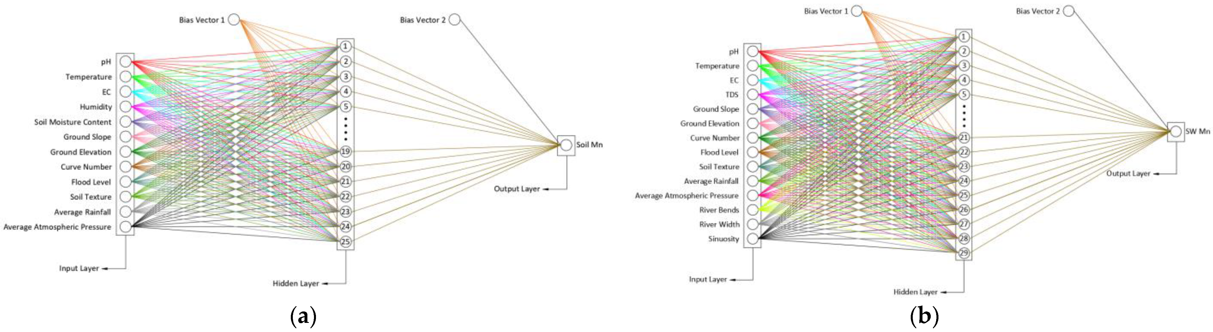
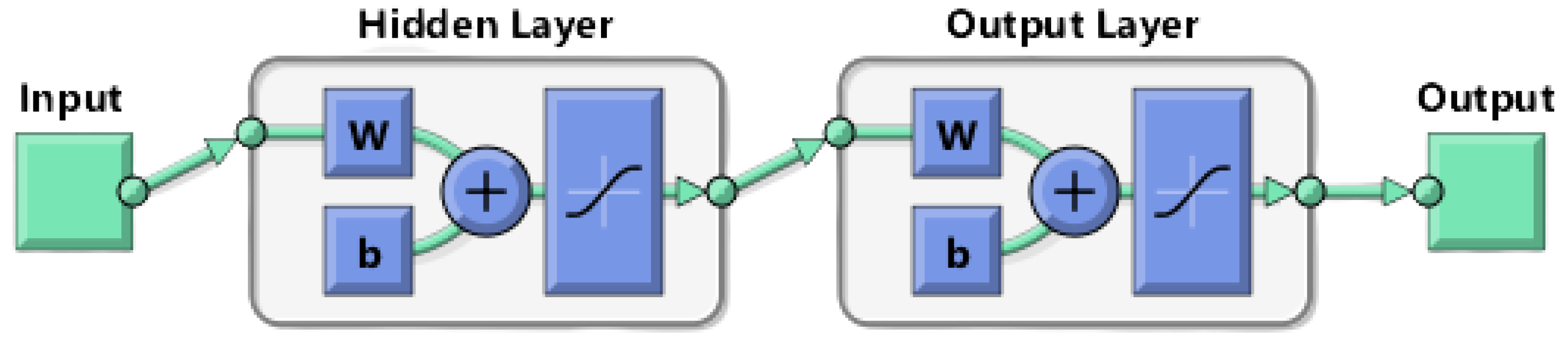
2.3.3. Artificial Neural Network Modelling

ANN is a machine-learning approach that mimics the function of a real biological neuron in the prediction and forecasting of complicated systems. ANN has been used in different environmental studies to provide reliable results in the assessment and prediction of contaminants in media, such as water [61], air [62], and soil [63]. The prediction capability of an ANN model relies on the dataset training quality. Datasets with known input and output parameter values are used to train the model, with ANN then identifying the relationship and patterns between input and output [64]. Backpropagation neural network learning is a subset of supervised learning that focuses on error minimization in this study. It needs a training dataset with a defined output and uses training to reduce the discrepancy between the projected output and the actual output [65]. The architecture of the ANN model is shown in Figure A1 in Appendix A.

In this study, the ANN models were created with MATLAB R2021a following the architecture as presented in Figure 5a,b for So and SW. The network type used was feed-forward backdrop, while Levenberg–Marquardt was chosen as the training algorithm due to its time efficiency in training moderate-sized feed-forward neural network models [66], with the Learn Gradient Descent with Momentum weight for the adaption learning function. The developed model used a hyperbolic tangent sigmoid (tansig) as the transfer function to connect the weight of the neuron with the input elements in the model. Complete internal characteristics of the ANN model used are presented in

Table 1. Simulation environment used in the ANN model.

Internal Characteristic	Max
Network Type	Feed-forward backdrop
Training Algorithm	Levenberg–Marquardt
Learning Function	Gradient descent with momentum weight and bias
Performance Function	Mean Squared Error
Transfer Function	Hyperbolic Tangent Sigmoid
Number of Layer	2
Hidden Neurons	25, 29

. All the datasets in this study that were extracted from the spatial grid maps (i.e., 563 soil + 117 SW 2019 + 117 SW 2021) were divided for the training and validation steps, with 85% of the data used to train the model, and 15% of the data used for external validation (see Figure 3) [67]. The network structure followed the equation 2m + 1, wherein “m” is the number of hidden neurons, as suggested in the study by Law et al. (in 2020) [68]. According to Nguyen et al. [69], excessive numbers of training datasets could lead to overfitting and provide erroneous results, thereby suggesting that training should not use all datasets and a portion should be left for validation.

2.3.4. Correlation Analysis of Identified Parameters and Feature Reduction

Correlation analysis was performed using Pearson correlation on all identified parameters for both soil and SW (input) and Mn concentration (output) to identify the degree of relationship [70]. The respective correlation between each input parameter and output Mn establishes how critical it would be in the developed ANN prediction model [71].

Feature reduction was also performed by reducing the number of input parameters in the training of the model. The input parameters for soil and SW were removed one by one, with the removal order based on the degree of correlation between input parameters and Mn (i.e., input parameter with the lowest degree of correlation would be removed first, and so on). This parameter reduction was performed to assess how the prediction model would perform with less input parameters [72], which may replicate the scenario at some sites or site areas where data and parameters are more limited and determine which parameters are critical and which can be neglected. For each scenario, parameter reduction was performed prior to model training.

2.3.5. Performance Evaluation

Performance evaluation of the ANN model is very important to determine the reliability of its prediction ability [73]. It can show whether the model is performing as desired or if it needs to undergo further training. The correlation coefficient (R) and mean squared error (MSE) were utilized to assess the performance of the soil ANN and SW ANN models during training within MATLAB. The R value indicates the performance of the network generalization and signals training termination when generalization ceases to improve. Both R and MSE were used by the model as basis in terminating its iteration or training. R and MSE can be seen as Figure A2 and Figure A3 in Appendix A.

In this study, the mean absolute percentage error (MAPE) was also computed to identify the average error of the model via comparison of the predicted value with the actual/measured value (see Equation (1)). Jierula et al. [74] evaluated a range of equations for measuring the accuracy of prediction models and indicated that MAPE is one of the best and most logical methods to employ.

$$MAPE=\frac{measured value-predicted value}{measured value}\times 100\%$$

(1)

The root mean squared error (RMSE) was also computed to provide the standard deviation of the residuals or prediction errors of the model. Using Euclidean distance, RMSE shows how far predictions are from measured values [75], as shown in Equation (2).

$$RMSE=\sqrt{\frac{{\sum }_{i=1}^N‖y\left(i\right)-\widehat{y}({i)‖}^2}{N}}$$

(2)

where N is the number of data points, $y$(i) is the i-th measurement, and $\widehat{y}$(i) is the predicted value.

Willmott’s Index was also used as an extra criterion to assess how well the created ANN models performed, as shown in Equation (3). Willmott’s Index, which ranges from 0 to 1, with 1 being the optimum value signifying an excellent match, is a metric of the agreement for the systematic evaluation of the extent of model prediction error. The index is able to calculate the proportional and cumulative differences between actual and forecasted averages and variances, but it is also excessively susceptible to extreme values because of squared disparities [76,77].

$$WI=1-\left[\frac{{\displaystyle \sum _{i=1}^N{\left(M{n}_{predicted}-M{n}_{observed}\right)}^2}}{{\displaystyle \sum _{i=1}^N{\left(\left|M{n}_{predicted}-\overline{M{n}_{observed}}\right|+\left|M{n}_{observed}-\overline{M{n}_{observed}}\right|\right)}^2}}\right]$$

(3)

3. Results

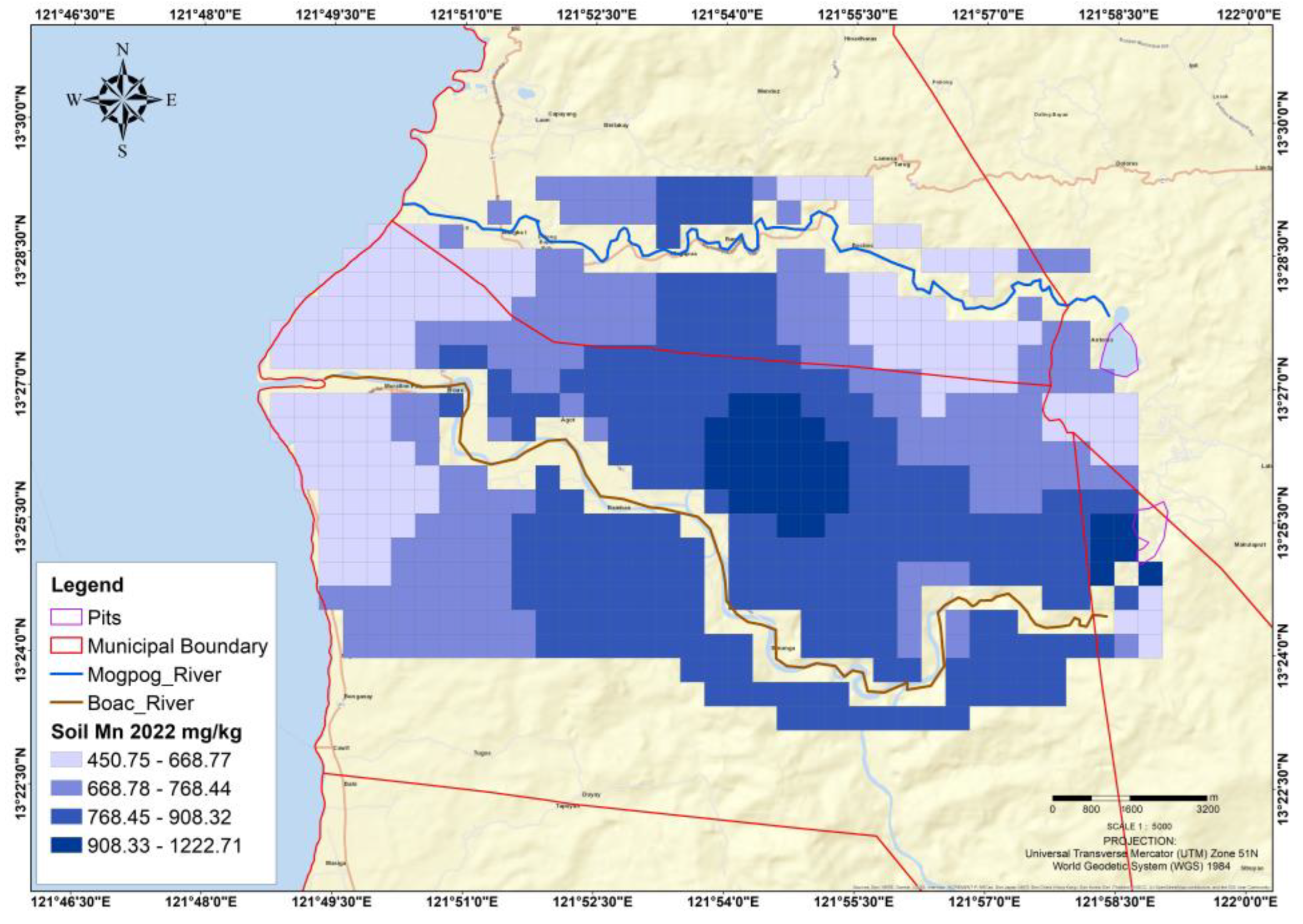
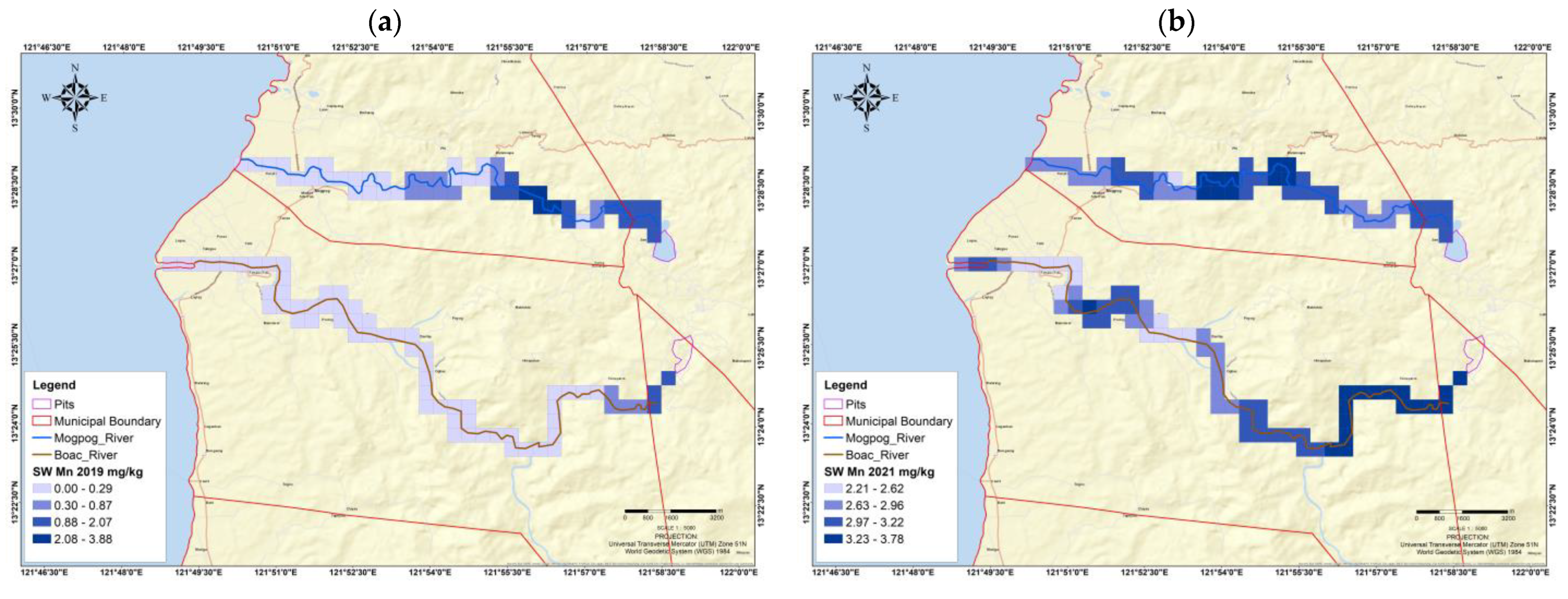
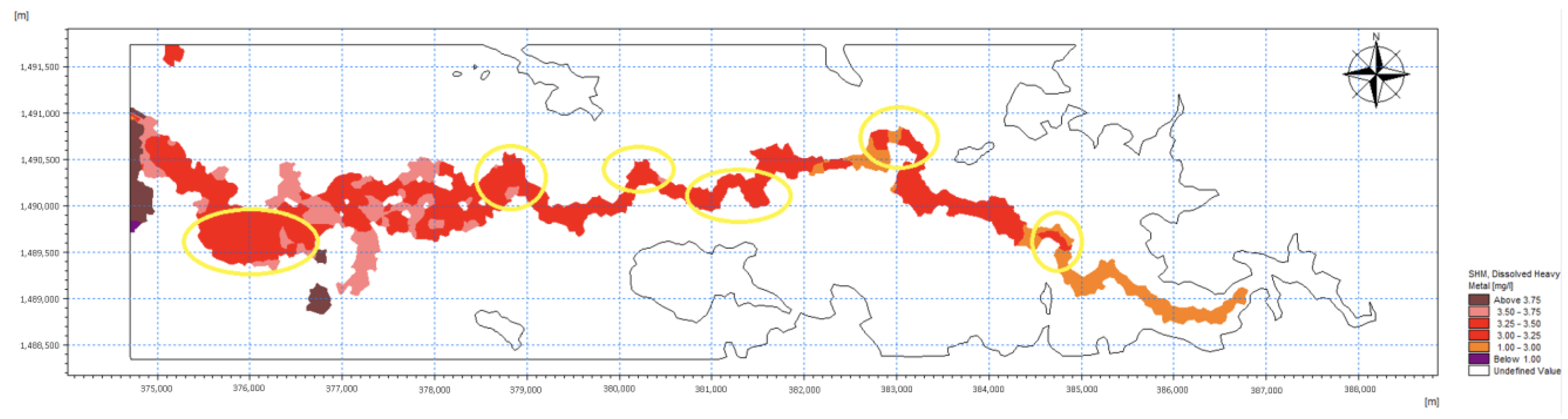
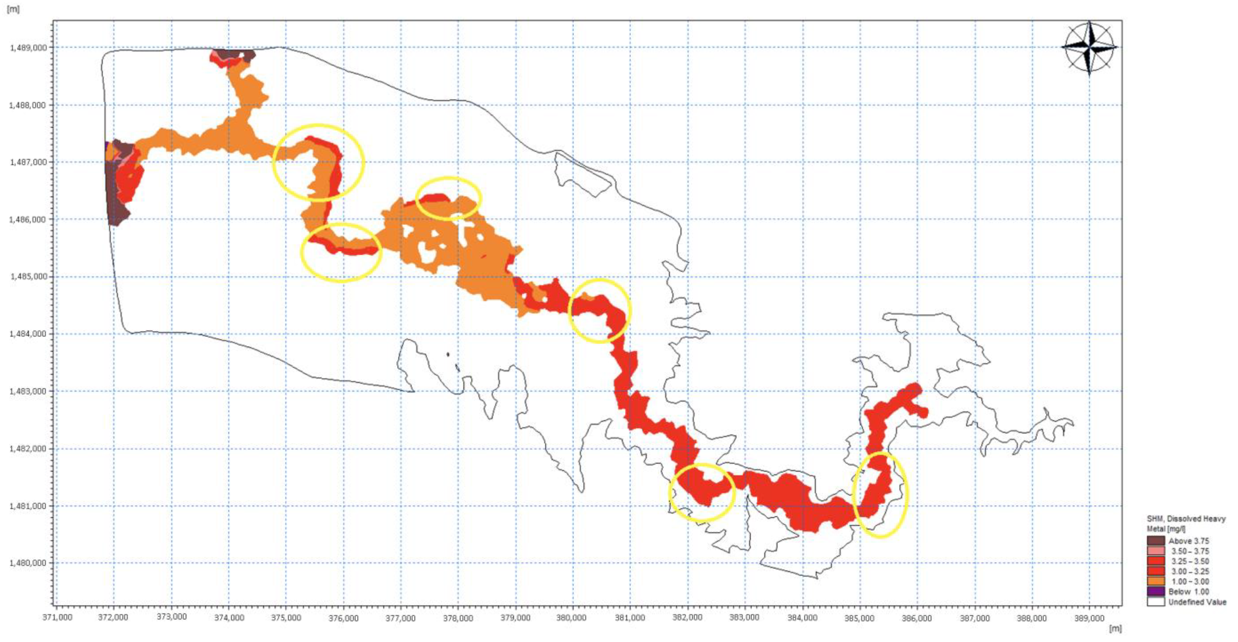
3.1. Spatial Grid Maps for Soil and SW

Figure 6 and Figure 7 present the spatially interpolated grid maps for soil and SW Mn concentrations, respectively. Each grid node illustrates the associated Mn concentration, ranging from low (light purple) to high (dark blue). Figure 5 shows that soil Mn concentration is higher in parts of Boac compared to Mogpog and highly concentrated near the pits. Figure 6 shows a higher concentration of SW Mn in the upstream regions and near the two pits. With this simple spatial analysis, it could be perceived that two mining pits are contributing a lot to the elevation of Mn in both soil and SW. The concentration of Mn in SW was also compared to the simulation performed using the MIKE Eco lab model as shown in Figure A4 and Figure A5 (Appendix A).

Results showed that accumulation happens mostly in the bends of the river and near the mining pits, providing more significance in considering the morphology of the river as an input parameter. While not shown here, each grid node also contains each input parameter with these datasets used in the ANN model. These datasets associated with the grid maps are summarized by descriptive statistics in

Table 2. Summary of descriptive statistics for all input parameters in the ANN model for soil.

Parameters	Max	Min	Mean	SD	Skewness	Kurtosis
Soil pH	6.282	3.193	5.251	0.641	−0.870	−0.246
Soil EC	593.715	98.758	308.565	65.105	1.101	2.623
Soil Humidity	124.069	12.654	27.682	12.700	3.100	15.554
Soil Temp	31.938	25.239	27.965	1.291	0.887	0.188
Soil MC	100.000	8.548	27.540	13.671	3.316	13.798
Ground Slope	29.284	2.252	13.610	5.587	0.041	−0.474
Ground Elevation	526.593	8.378	183.195	124.954	0.461	−0.695
CN	92.139	35.923	79.817	7.553	−1.803	5.835
Flood Level	3.000	1.000	1.086	0.288	3.192	9.333
Soil Texture	3.000	1.000	1.139	0.445	3.345	10.053
Rainfall	188.973	178.079	183.829	2.912	−0.146	−1.119
Atm. Temp	25.834	25.745	25.782	0.024	0.381	−0.944
Soil Mn	1222.710	450.750	757.698	111.224	0.584	1.580

and

Table 3. Summary of descriptive statistics for all input parameters in the ANN model for SW.

Parameters	Max	Min	Mean	SD	Skewness	Kurtosis
SW pH	8.381	3.652	6.903	0.944	−1.684	2.566
SW EC	4094.130	113.617	781.436	455.648	3.550	16.932
SW TDS	2032.230	51.636	380.204	227.379	3.545	16.862
SW Temp	34.320	29.118	31.313	0.954	0.298	0.066
Ground Slope	28.052	2.601	11.751	6.692	0.380	−1.056
Ground Elevation	365.968	8.978	97.859	83.287	1.097	0.369
River Bends	4.000	0.000	1.971	1.008	0.197	−0.624
Width	261.750	57.213	138.472	67.436	0.416	−1.227
Sinuosity	1.924	1.000	1.339	0.254	0.709	−0.461
CN	92.973	36.193	73.982	14.235	−0.988	−0.242
Flood Level	3.000	1.000	1.371	0.518	0.917	−0.364
Soil Texture	3.000	1.000	1.549	0.783	0.972	−0.800
Rainfall	473.605	354.518	411.147	50.359	0.023	−1.961
Atm. Temp	27.773	26.670	27.222	0.521	−0.001	−2.008
SW Mn	3.884	0.002	1.714	1.409	−0.134	−1.833

.

Table 2 presents the descriptive statistics for the 12 selected input parameters for soil that have potential correlation to Mn. Soil pH and EC have previously been correlated to increased metal concentrations [78], with higher pH shown to promote higher Mn concentration in soils since alkalinity of soils reduces Mn availability to plants [79]. In this study, soil pH ranged from 3.19 to 6.28, while the average EC for the whole area was 308.565 mS/cm, with a higher standard deviation (SD) indicating higher variability of EC throughout the area. Soil temperature can greatly affect the accumulation of metals in plants and also affect the availability of metals in soil during this process. According to Lee et al. [80], increasing soil temperatures also increases the soil-to-plant transfer of heavy metals. The average soil temperature in Mogpog and Boac was 28.0 °C, with a SD of 1.3. Ground elevation and ground slope were also considered as input parameters since the terrain of an area can affect the spatial distribution of heavy metals in soils [81]. The highest elevation in the study was 526.59 masl, while the highest slope was 29.3°. As these values are based in the terrain, they do not really change with time.

The CN and flood level have also been correlated to Mn in soil [82], with CN related to the capability of soil to be infiltrated by water, and flood level indicating the extent and level of floods that these soils are subjected to. Average CN in the study area was 79.82, while the average normalized value for flood level was 1.09, which is equivalent to 0.136 m. The corresponding actual value of flood level is shown in

Table A1. Summary of the flood level codes related to flood height.

FL Code	Flood Height
0–1	No flood
1–2	0.1–0.5 m
2–3	0.5–1.5 m
Above 3	Above 1.5 m

in Appendix A. Soil texture is also a normalized value that corresponds with 1-clay loam, 2-sand, and 3-sandy loam. Average soil code in the study area was 1.14, indicating that the majority of soil in Mogpog and Boac is clay loam. Climate change occurs everywhere and can affect metal transport in catchment areas [32]. This study includes the possible effect of climate change by considering both rainfall and atmospheric temperature. The highest rainfall in the area was 188.97 mm, with a small SD. Similarly, atmospheric temperature in the area showed little deviation, with its highest value of 25.8 °C and lowest value of 25.7 °C. Finally, Table 3 shows that the highest concentration of Mn in soil was 1222.7 mg/kg, with an average concentration of 757.7 mg/kg for the whole area.

Table 3 presents the descriptive statistics for the 14 input parameters for SW that may be correlated to SW Mn. The physicochemical properties of water, such as pH, temperature, EC, and TDS, have long been used in studies due to their relationship to metal contamination [12,83]. The pH is critical as metals are more soluble in acidic water [84], while the pH also affects the adsorption–desorption process in sediments [85]. In this study, the lowest SW pH was 3.65, which was located in areas nearest to the open mine pits [82]. EC and TDS have values directly correlated to one another, with average readings for EC and TDS equal to 781.4 mS/cm and 380.2 mg/L, respectively [86]. Ground elevation and ground slope have also been shown to affect SW quality. Ground elevation ranged from 8.98 masl to 365.968 masl, highlighting the difference in elevation between upstream and downstream portions of the rivers, which can strongly influence its flow velocity. Ground slope has an average value of 11.75°, which can also affect the velocity of flow and retention of SW in the river channel.

In contrast to the ANN model for soil, the ANN model for SW is applied to river systems and influenced by its hydrodynamics. The morphological parameters of the river, such as river bends, width, and sinuosity, were measured for this study. River bends [87] and sinuosity [23] control how sediments can accumulate along a river channel and act like a storage facility for metals that can be stored and released depending on environmental conditions. The average number of river bends within each grid node in this study was 1.97, with an average sinuosity of 1.34, with these values considered significant to induce sediment accumulation. The average river width was 138.5 m. Similar to the ANN model for soil, CN, flood level, soil code, rainfall average, and atmospheric temperature were also considered for the SW model, with average values of 73.98, 1.371 (0.1–0.5 m), 1.549 (clay loam), 411.15 mm, and 27.2 °C, respectively. The average concentration of Mn in SW was 1.71 mg/L, with a maximum value of 3.88 mg/L located nearest to the mine pits.

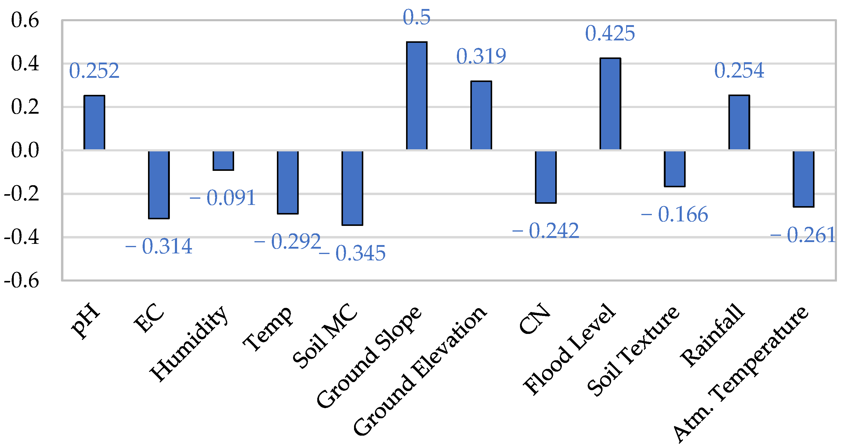
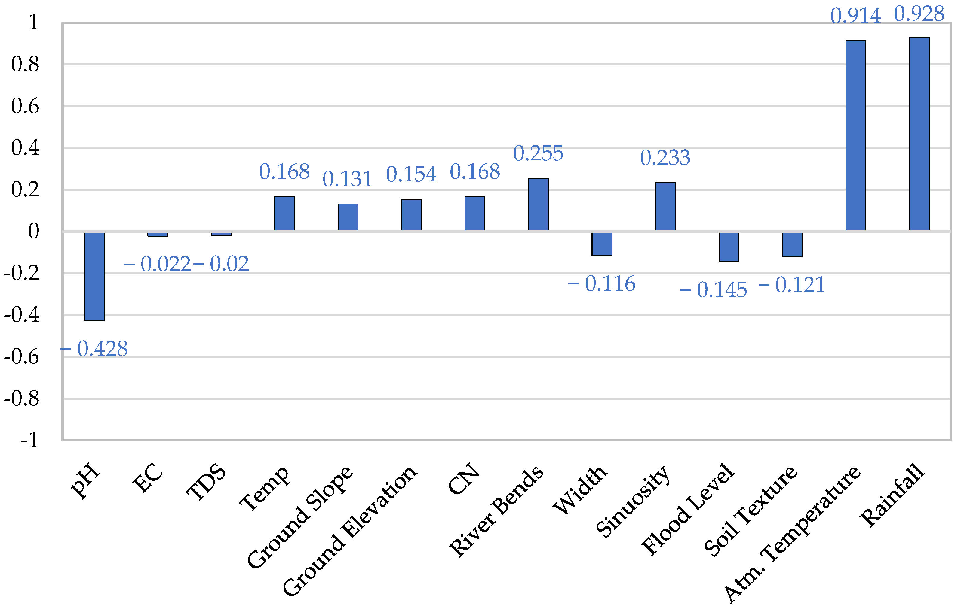
3.2. Correlation Analysis

Figure 8 presents the degree of correlation for each of the 12 input parameters for soil to the output parameter (soil Mn). Each parameter has a different degree of correlation, whether it is direct or inverse. Ground slope has the highest correlation value of 0.499, while humidity has the lowest with −0.091. It is noted that correlation of soil pH (0.252) and rainfall (0.254) are very similar, as soil pH is known to decrease over time due to leaching caused by high amounts of rainfall that produce acidification [86]. As shown in Figure 7, the degree of correlation from highest to lowest for all parameters is as follows: Ground Slope > Flood Level > Soil MC > Ground Elevation > EC > Soil Temperature > Atmospheric Temperature > Rainfall > Soil pH > CN > Soil Texture > Humidity. All correlation values for each parameter are provided in

Table A2. Degree of correlation between each soil input parameter and soil Mn.

	pH	EC	Hum	Temp	Mo	Sl	El	CN	Fl	ST	Rave	Tave	So Mn
pH	1.000
EC	0.476	1.000
Hum	0.175	0.508	1.000
Temp	−0.632	−0.397	−0.342	1.000
Mo	0.355	0.815	0.485	−0.386	1.000
Sl	−0.093	−0.441	−0.142	−0.172	−0.452	1.000
El	−0.348	−0.639	−0.391	0.241	−0.496	0.587	1.000
CN	−0.301	−0.043	0.012	0.373	−0.061	−0.086	0.125	1.000
Fl	0.130	−0.036	−0.050	−0.177	−0.028	0.075	0.063	−0.034	1.000
ST	0.235	0.211	0.026	−0.220	0.252	−0.393	−0.345	−0.548	−0.062	1.000
Rave	−0.677	−0.727	−0.369	0.477	−0.555	0.405	0.738	0.265	0.069	−0.342	1.000
Tave	0.677	0.666	0.287	−0.409	0.485	−0.391	−0.709	−0.263	−0.086	0.324	−0.989	1.000
Soil Mn	0.252	−0.314	−0.091	−0.292	−0.345	0.500	0.319	−0.242	0.425	−0.166	0.254	−0.261	1.000

.

Figure 9 presents the degree of correlation between each of the 14 SW input parameters and the Mn concentration in SW. Average rainfall received in the area was found to have the highest correlation of 0.928 since it can be related to the overflow from the two open mine pits during rainfall events [21]. This crucial parameter can also control future contamination in the area due to the continuous existence of the pits. SW pH also has a significant correlation of −0.428 since it is known that acidic water can induce desorption of metals from sediments, making them more soluble [84,85]. The lowest correlation was SW TDS (−0.019) since TDS can also be affected by saltwater intrusion unrelated to Mn and/or discharge from the open pits. It is also evident from

Table A3. Degree of correlation between each SW input parameter and SW Mn.

	pH	EC	TDS	Temp	Sl	El	CN	RB	W	Si	Fl	ST	Tave	Rave	SW Mn
pH	1.000
EC	−0.168	1.000
TDS	−0.164	0.998	1.000
Temp	0.352	−0.124	−0.108	1.000
Sl	−0.327	0.025	0.017	−0.447	1.000
El	−0.403	0.077	0.091	−0.427	0.751	1.000
CN	−0.487	0.024	0.023	−0.147	0.216	0.229	1.000
RB	−0.482	0.105	0.099	−0.080	0.128	0.143	0.438	1.000
W	0.409	−0.282	−0.277	0.403	−0.314	−0.361	−0.390	−0.458	1.000
Si	−0.404	0.137	0.131	−0.165	0.243	0.222	0.384	0.602	−0.396	1.000
Fl	0.156	−0.228	−0.220	0.168	−0.432	−0.315	−0.098	−0.031	0.141	−0.075	1.000
ST	0.470	0.002	−0.006	0.228	−0.389	−0.393	−0.871	−0.465	0.442	−0.426	0.107	1.000
Tave	−0.266	−0.052	−0.062	0.190	0.021	−0.010	0.077	0.164	0.120	0.145	−0.067	0.005	1.000
Rave	−0.041	−0.108	−0.112	0.280	−0.047	−0.053	−0.059	0.065	0.176	0.006	−0.003	0.083	0.903	1.000
SW Mn	−0.428	−0.022	−0.020	0.168	0.131	0.154	0.168	0.255	−0.116	0.233	−0.145	−0.121	0.914	0.928	1.000

that river morphology affects Mn accumulation in SW, with sinuosity and river bend values of 0.223 and 0.255, respectively. The degree of correlation from highest to lowest is Rainfall > Atmospheric Temperature > SW pH > River Bends > Sinuosity > SW Temperature > CN > Ground Elevation > Flood Level > Ground Slope > Soil Texture > River Width > SW EC > SW TDS. The correlation values for each parameter are shown in Table A3.

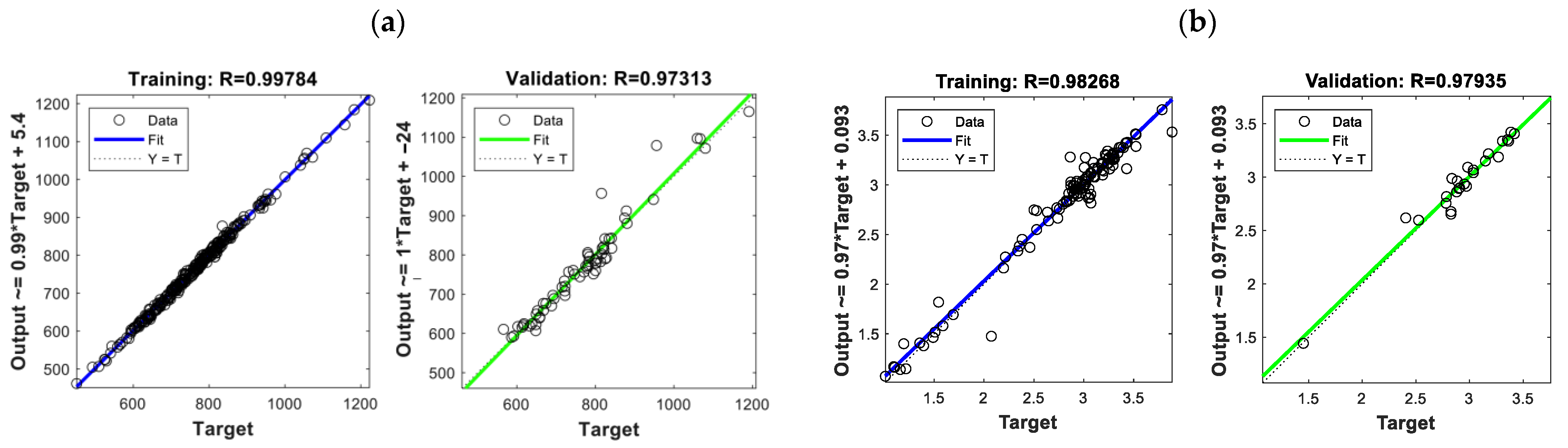
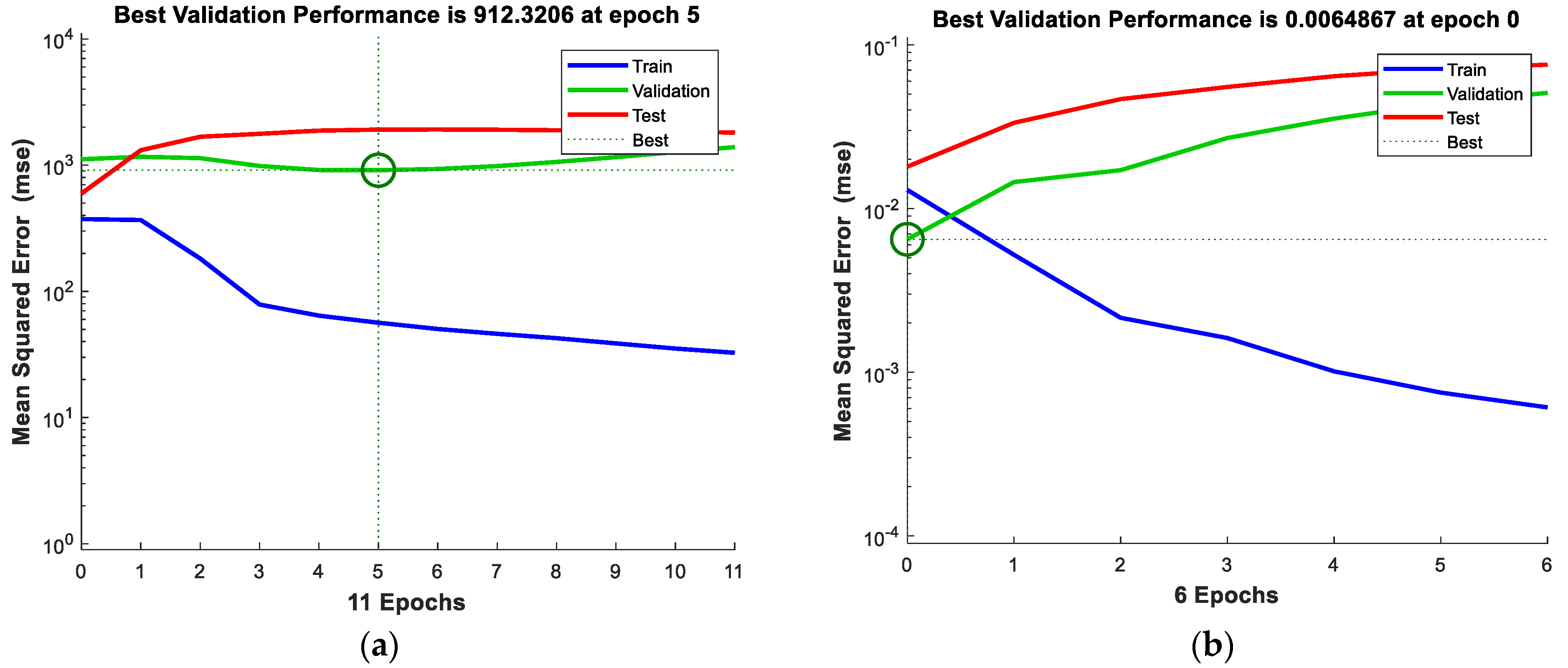
3.3. ANN Modelling and Feature Reduction

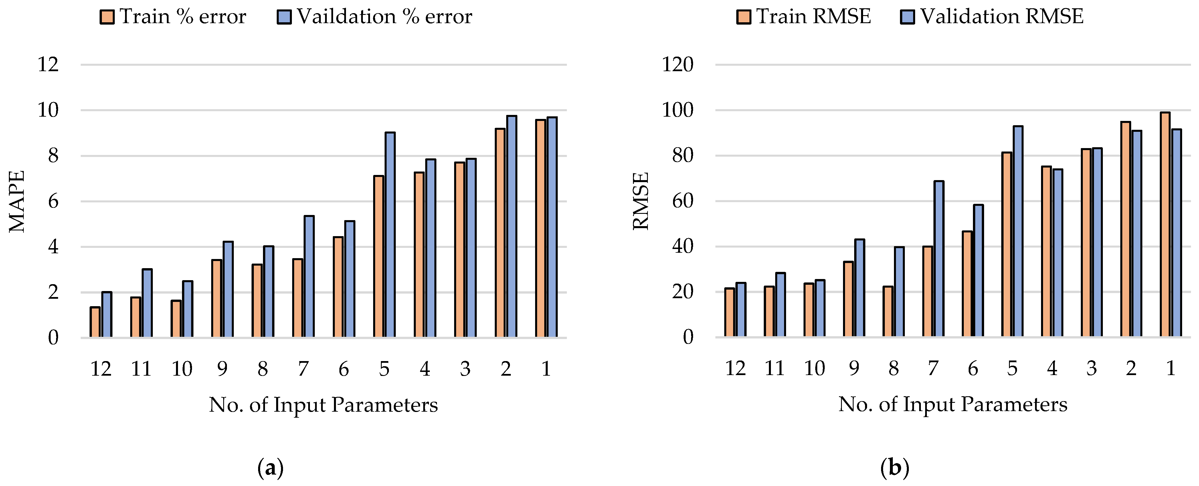
3.3.1. ANN Model for Soil and Feature Reduction Analysis

The ANN model for soil Mn was first trained for the scenario with 12 input parameters, with the training of the model continually repeated until the minimum gradient was reached and the result stopped changing. The model was then validated with an unbiased comparison of the trained model results (output Mn) with actual results (field-measured Mn). Figure 10a presents the performance evaluation results of the ANN model for 12 inputs (leftmost bars) in terms of MAPE for training (orange) and validation (blue). The MAPE value was lower for training (1.34%) than validation (3.01%). It is logical that the MAPE value is lower for training since the training datasets were directly used in the actual training itself and had a model bias, unlike the validation datasets.

The ANN model training and validation were then repeated for decreasing numbers of input parameters. The order for the one-by-one removal of input was based on the degree of correlation values in Table A3 and

Table A4. Summary of results for the feature reduction analysis in the ANN model for soil Mn.

Input Parameters	Train		Validation
	%Error	RMSE	%Error	RMSE	Features Reduced
12	1.343	21.535	2.01	23.979	None
11	1.779	22.327	3.016	28.303	Hum
10	1.637	23.656	2.494	25.210	Hum, ST
9	3.423	33.236	4.231	43.133	Hum, ST, CN
8	3.223	22.360	4.025	39.728	Hum, ST, CN, pH
7	3.459	39.980	5.351	68.714	Hum, ST, CN, pH, Rave
6	4.430	46.577	5.130	58.294	Hum, ST, CN, pH, Rave, Tave
5	7.114	81.418	9.020	92.894	Hum, ST, CN, pH, Rave, Tave, Temp
4	7.271	75.205	7.843	73.951	Hum, ST, CN, pH, Rave, Tave, Temp, EC
3	7.710	82.912	7.871	83.253	Hum, ST, CN, pH, Rave, Tave, Temp, EC, El
2	9.187	94.868	9.756	90.994	Hum, ST, CN, pH, Rave, Tave, Temp, EC, El, Mo
1	9.581	98.963	9.694	91.525	Hum, ST, CN, pH, Rave, Tave, Temp, EC, El, Mo, Fl

(i.e., ground slope had the lowest correlation and was removed first to run the scenario with 11 input parameters). Figure 10a also presents the MAPE performance evaluation results for each of the reduced input parameter model scenarios. It shows that the training and validation of the ANN model gradually decline in performance with the reduction in input parameters, with the highest MAPE and values for training (9.58%) and validation (9.69%) occurring when only one input parameter is used. There is no specified allowable MAPE value to evaluate prediction models; it will always be dependent on the intended application of the model. Shi et al. [86] developed machine learning models with seven input parameters for heavy metal estimation in soils, and despite having an average MAPE of 12.14%, the prediction model was wholly sufficient for metal estimation in their study [86].

RMSE was also computed for each model scenario to identify how much predicted values deviate from the actual value [75], with lower RMSE values indicating higher model estimation accuracy [86]. As shown in Figure 10b, the lowest RMSE computed in the training and validation steps for the model with 12 input parameters was 21.54 mg/kg and 23.98 mg/kg, respectively. As shown in Table 2, the average Mn in soil was 757.7 mg/kg, so obtaining an RMSE of 23.98 in external validation can be considered acceptable given the high range of values. The highest RMSE was found in the model scenario with a single input parameter, with only values of 98.96 and 91.53 for training and validation, respectively.

These ANN model results indicate that Mn in soil can be best predicted using the model with all 12 input parameters. However, the models with 11, 10, 9, and 8 input parameters still provide MAPE values of <5% in the external validation. This suggests that even if humidity, soil texture, CN, and soil pH are not available, the model could still provide sufficient estimates of Mn concentration in soil. The detailed results of the soil ANN model are presented in Table A4.

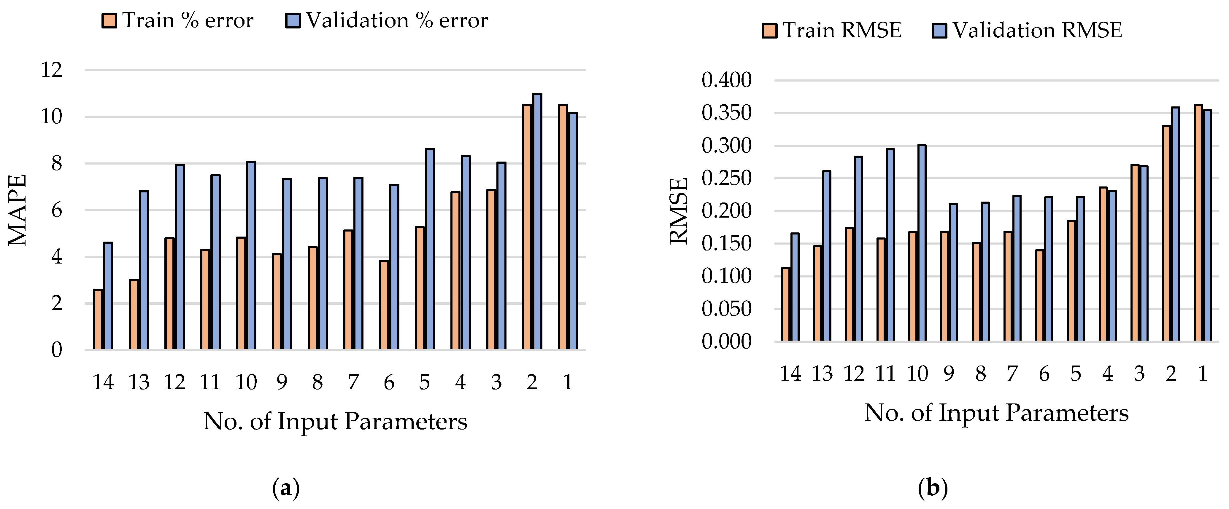
3.3.2. ANN Model for SW and Feature Reduction Analysis

The ANN model for predicting SW Mn from all 14 input parameters did not initially produce a good prediction model, with MAPE values of 38.34% and 154.00% in the training and validation steps, respectively. Due to this poor performance, two ANN models for SW Mn were developed based on ranges of SW Mn values, which has been shown to provide better results if combining all SW values together did not work [87]. The SW data were divided into two groups for these two models based on the range of Mn in SW. The first model used SW Mn values within the 0–1 mg/L range, obtaining MAPE values of 13.55% and 85.95% for the training and validation steps, respectively. The second model used SW Mn values >1 mg/L, achieving MAPE values of 2.59% and 4.61%, respectively.

Figure 11 presents the performance evaluation results of the ANN model for predicting SW Mn, where only Mn values >1 mg/L were considered. Similar to the soil Mn model, the lowest MAPE and RMSE were achieved with all 14 input parameters. This indicates how important both the chemical properties of SW and the physical properties of the river are to best predict Mn concentration in SW. The MAPE for this scenario was 2.59% and 4.61% for the training and validation steps, respectively. Again, the model with a single input parameter had the lowest performance, with the MAPE for training and validation equal to 10.52% and 10.18%, respectively. The full details of the ANN model for SW Mn are presented in

Table A5. Summary of results for the feature reduction analysis in the ANN model for SW Mn.

Input Parameters	Train		Validation
	%Error	RMSE	%Error	RMSE	Features Reduced
14	2.590	0.113	4.609	0.166	None
13	3.012	0.146	6.808	0.261	TDS
12	4.795	0.174	7.933	0.283	TDS, EC
11	4.298	0.158	7.506	0.295	TDS, EC, W
10	4.828	0.168	8.075	0.301	TDS, EC, W, ST
9	4.106	0.169	7.334	0.210	TDS, EC, W, ST, Sl
8	4.415	0.151	7.387	0.213	TDS, EC, W, ST, Sl, Fl
7	5.126	0.168	7.391	0.223	TDS, EC, W, ST, Sl, Fl, El
6	4.212	0.140	7.086	0.221	TDS, EC, W, ST, Sl, Fl, El, CN
5	5.266	0.185	8.625	0.221	TDS, EC, W, ST, Sl, Fl, El, CN, Temp
4	6.762	0.236	8.330	0.230	TDS, EC, W, ST, Sl, Fl, El, CN, Temp, Si
3	6.862	0.271	8.045	0.269	TDS, EC, W, ST, Sl, Fl, El, CN, Temp, Si, RB
2	10.512	0.330	10.986	0.359	TDS, EC, W, ST, Sl, Fl, El, CN, Temp, Si, RB, pH
1	10.521	0.363	10.175	0.354	TDS, EC, W, ST, Sl, Fl, El, CN, Temp, Si, RB, pH, Rave

.

Utilizing the observed and predicted values of the Mn concentrations for the soil and SW models, the WI values for the soil Mn and SW Mn models are 0.996 and 0.998, respectively. These values indicate the efficiency and reliability of the developed soil and SW Mn models since the calculated values were approaching the ideal value of 1. This provides an additional layer of validation for the prediction model developed in this study.

4. Discussion

ANN models have become highly popular in environmental studies [12,88] due to their extensive capabilities to solve complex problems [89]. In this study, ANN was employed to create prediction models for Mn in soil and SW. Previous studies have developed prediction models but only included a limited number of input parameters that did not combine chemical with physical parameters. In this study, extensive data were collected and analyzed to create datasets that can be used for the training and validation of the two ANN models for soil Mn and SW Mn.

The soil Mn model used 12 input parameters varying in their degree of correlation to Mn, with ground slope having the highest correlation (r = 0.500) and humidity having the lowest (r = −0.091). Similarly, the 14 input parameters for the SW Mn model were arranged according to their correlation with SW Mn. SW Mn is highly correlated to rainfall in the area (r = 0.928), which can be associated with the overflow of the contaminants from the open mine pits to the Mogpog and Boac Rivers [21,35,36,45,46]. SW pH was also highly correlated to Mn concentration (r = −0.428). According to Saalidong et al. [84], lower pH could stimulate the desorption of metals from sediments in rivers [84]. This also highlights the importance of river morphology as it controls sediment deposition [22], which can also contribute to elevated Mn in the area.

Performance evaluation of both models [74,90,91] confirmed their prediction accuracy, with MAPE values of <5%, even lower than acceptable values in other studies [86,91,92,93]. The feature reduction for each ANN model helped to identify how each model responded when certain input parameters were removed. Previous studies have used this approach to assess whether and which parameters can be removed to improve model accuracy [94]. The two ANN models for soil Mn and SW Mn achieved the highest performance when all possible input parameters were included, highlighting the influence of each parameter on Mn accumulation that has been demonstrated in a wealth of studies [21,32,78,79,80,81]. Nevertheless, the feature reduction did demonstrate that the prediction models can still provide sufficient accuracy even if 4–5 input parameters were excluded from the model training. The trained and validated ANN models can provide a more accessible and less expensive strategy for environmental monitoring. The ANN models developed in this study are useful to LGUs, communities, researchers, engineers, and scientists who are monitoring the SW and soil quality. Moreover, these models are beneficial in areas and neighboring countries with similar environmental conditions that need to be monitored. Basic and easier-to-measure in situ parameters, such as pH, EC, river morphology, and rainfall, can be used to predict Mn concentrations. These models are important to communities in remote and less developed areas, such as the study site on the island of Marinduque. Adjusting input parameter values and predicting their effect on Mn concentrations can be very beneficial to help local authorities design and implement more efficient mitigation strategies.

The model developed in this study should be continually refined, especially with future advances in machine-learning approaches [95]. New algorithms in neural networks are expected to improve the prediction accuracy of the models. Furthermore, the model approach in this study can be extended to predict the concentration of other heavy metals and contaminants in the environment and could also be used for projections that consider the effect of climate change since climate data are one of the inputs of the model. Future work could consider developing a model for different species of Mn as it could react differently with other identified parameters.

5. Conclusions

The areas surrounding the Mogpog and Boac Rivers on the island of Marinduque in the Philippines have been contaminated with toxic mine tailings from the two abandoned open mine pits. The Mn concentrations in soil and SW were well above standard limits, with values of 1222.7 mg/kg and 3.884 mg/L, respectively. Unfortunately, local communities were unaware of the associated risks and continue to rely on SW from the rivers and adjacent agricultural lands for everyday needs. Soil and SW quality should be better monitored; however, expertise and funds to support the needed monitoring activities of more complex parameters of heavy metals is a challenge in many areas including the islands of the Philippines. This motivated the need to develop a model with ANN to predict Mn concentrations in the environment, specifically in soil and SW, from correlated parameters that can be measured more easily.

ANN models were developed to predict Mn in soil and SW, using 12 and 14 input parameters, respectively, that were extracted from spatial grid maps of the study area. The ANN model for soil Mn achieved MAPE values of 1.34% and 2.01% for the training and external validation steps of the model development, respectively. The SW Mn model was split into two models based on SW concentrations ranges of 0–1 mg/L and >1 mg/L. The model for the 0–1 mg/L SW Mn range achieved MAPE values of 13.55% and 85.95% for training and validation, respectively, while the model for the >1 mg/L SW Mn range achieved MAPE values of 2.59% and 4.61% for training and validation, respectively. The ANN models were also trained and validated with successive reductions in the number of input parameters to investigate whether such an extensive list of parameters is always necessary. To determine the order in which the input parameters were removed, the degree of correlation between each parameter and the concentration of Mn in soil and SW was first calculated. For soil Mn, ground slope had the highest correlation (r = 0.500), followed by flood level (r = 0.425), while the lowest correlation was found with soil humidity. For SW Mn, rainfall had the highest correlation (r = 0.928), which can be expected as it directly contributes to overflow from the mine pits, with EC and TDS having the lowest correlation, which may occur due to the influence of salinity from saltwater intrusion. The ANN models with reduced input parameters did diminish the accuracy of the model predictions relative to the initial scenarios with 12 and 14 input parameters; however, sufficient accuracy can still be obtained if certain parameters are removed or retained. For example, the ANN model for soil Mn maintained a MAPE value <5% even when the input parameters were reduced from 12 to 8.

References

1. Tóth, G.; Hermann, T.; da Silva, M.R.; Montanarella, L. Monitoring Soil for Sustainable Development and Land Degradation Neutrality. Environ. Monit. Assess. 2018, 190, 57. [Google Scholar] [CrossRef] [PubMed] [Green Version]
2. Why Monitor Water Quality? Available online: https://water.usgs.gov/owq/WhyMonitorWaterQuality.pdf (accessed on 22 February 2023).
3. Ahuja, S. Monitoring Water Quality: Pollution Assessment, Analysis, and Remediation, 1st ed.; Elsevier: Amsterdam, The Netherlands, 2013. [Google Scholar]
4. Bhagwat, V.R. Safety of Water Used in Food Production. In Food Safety and Human Health; Elsevier: Amsterdam, The Netherlands, 2019; pp. 219–247. [Google Scholar]
5. Askari, M.S.; O’Rourke, S.M.; Holden, N.M. Evaluation of Soil Quality for Agricultural Production Using Visible–near-Infrared Spectroscopy. Geoderma 2015, 243–244, 80–91. [Google Scholar] [CrossRef]
6. FAO Initiative Brings Global Land Cover Data under One Roof for the First Time. Available online: https://www.fao.org/news/story/en/item/216144/icode/#:~:text=artificial%20surfaces%20(which%20cover%200.6,grasslands%20(13.0%20percent) (accessed on 22 February 2023).
7. Where Is Earth’s Water? Available online: https://www.usgs.gov/special-topics/water-science-school/science/where-earths-water#:~:text=Almost%20all%20of%20it%20is,serves%20most%20of%20life’s%20needs (accessed on 22 February 2023).
8. Environmental Monitoring. Available online: https://unece.org/environmental-monitoring (accessed on 22 February 2023).
9. Biber, E. The Challenge of Collecting and Using Environmental Monitoring Data. Ecol. Soc. 2013, 18, art68. [Google Scholar] [CrossRef] [Green Version]
10. Kirschke, S.; Avellán, T.; Bärlund, I.; Bogardi, J.J.; Carvalho, L.; Chapman, D.; Dickens, C.W.S.; Irvine, K.; Lee, S.; Mehner, T.; et al. Capacity Challenges in Water Quality Monitoring: Understanding the Role of Human Development. Environ. Monit. Assess. 2020, 192, 298. [Google Scholar] [CrossRef] [Green Version]
11. Huynh, T.-M.-T.; Ni, C.-F.; Su, Y.-S.; Nguyen, V.-C.-N.; Lee, I.-H.; Lin, C.-P.; Nguyen, H.-H. Predicting Heavy Metal Concentrations in Shallow Aquifer Systems Based on Low-Cost Physiochemical Parameters Using Machine Learning Techniques. Int. J. Environ. Res. Public. Health 2022, 19, 12180. [Google Scholar] [CrossRef]
12. De Jesus, K.L.M.; Senoro, D.B.; Dela Cruz, J.C.; Chan, E.B. Neuro-Particle Swarm Optimization Based In-Situ Prediction Model for Heavy Metals Concentration in Groundwater and Surface Water. Toxics 2022, 10, 95. [Google Scholar] [CrossRef]
13. Saxena, N.; Varshney, D. Smart Home Security Solutions Using Facial Authentication and Speaker Recognition through Artificial Neural Networks. Int. J. Cogn. Comput. Eng. 2021, 2, 154–164. [Google Scholar] [CrossRef]
14. Milačić, L.; Jović, S.; Vujović, T.; Miljković, J. Application of Artificial Neural Network with Extreme Learning Machine for Economic Growth Estimation. Phys. A Stat. Mech. Its Appl. 2017, 465, 285–288. [Google Scholar] [CrossRef]
15. Ogunsina, K.; Okolo, W.A. Artificial Neural Network Modeling for Airline Disruption Management. J. Aerosp. Inf. Syst. 2022, 19, 382–393. [Google Scholar] [CrossRef]
16. Shahid, N.; Rappon, T.; Berta, W. Applications of Artificial Neural Networks in Health Care Organizational Decision-Making: A Scoping Review. PLoS ONE 2019, 14, e0212356. [Google Scholar] [CrossRef]
17. Otake, R.; Kurima, J.; Goto, H.; Sawada, S. Deep Learning Model for Spatial Interpolation of Real-Time Seismic Intensity. Seismol. Res. Lett. 2020, 91, 3433–3443. [Google Scholar] [CrossRef]
18. Kakar, S.A.; Sheikh, N.; Naseem, A.; Iqbal, S.; Rehman, A.; Ullah, A.; Ahmad, B.; Ali, H.; Khan, B. Artificial Neural Network Based Weather Prediction Using Back Propagation Technique. Int. J. Adv. Comp. Sci. App. 2018, 9, 462–470. [Google Scholar] [CrossRef] [Green Version]
19. IBM: What Are Neural Networks. Available online: https://www.ibm.com/topics/neural-networks (accessed on 28 February 2023).
20. Kicińska, A.; Pomykała, R.; Izquierdo-Diaz, M. Changes in Soil pH and Mobility of Heavy Metals in Contaminated Soils. Eur. J. Soil. Sci. 2022, 73, e13203. [Google Scholar] [CrossRef]
21. Monjardin, C.E.F.; Senoro, D.B.; Magbanlac, J.J.M.; de Jesus, K.L.M.; Tabelin, C.B.; Natal, P.M. Geo-Accumulation Index of Manganese in Soils Due to Flooding in Boac and Mogpog Rivers, Marinduque, Philippines with Mining Disaster Exposure. App. Sci. 2022, 12, 3527. [Google Scholar] [CrossRef]
22. Xiao, C.; Chen, J.; Yuan, X.; Chen, R.; Song, X. Model Test of the Effect of River Sinuosity on Nitrogen Purification Efficiency. Water 2020, 12, 1677. [Google Scholar] [CrossRef]
23. Huang, H.; Chen, G.; Zhang, Q.F. Influence of River Sinuosity on the Distribution of Conservative Pollutants. J. Hydrol. Eng. 2012, 17, 1296–1301. [Google Scholar] [CrossRef]
24. Song, L.; Han, Z.; Li, Z.; Zhao, G.; Yang, R. Effects of Atmospheric Precipitation on Heavy Metal Accumulation and Deactivation Amendment in Wheat Around a Lead Smelter. Water Air Soil. Pollut. 2020, 231, 327. [Google Scholar] [CrossRef]
25. Dinić, Z.; Maksimović, J.; Stanojković-Sebić, A.; Pivić, R. Prediction Models for Bioavailability of Mn, Cu, Zn, Ni and Pb in Soils of Republic of Serbia. Agronomy 2019, 9, 856. [Google Scholar] [CrossRef] [Green Version]
26. Zhao, W.; Ma, J.; Liu, Q.; Dou, L.; Qu, Y.; Shi, H.; Sun, Y.; Chen, H.; Tian, Y.; Wu, F. Accurate Prediction of Soil Heavy Metal Pollution Using an Improved Machine Learning Method: A Case Study in the Pearl River Delta, China. Environ. Sci. Technol. 2023. [Google Scholar] [CrossRef]
27. Ahangar, A.G.; Soltani, J.; Abdolmaleki, A.S. Predicting Mn concentration in water reservoir using Artificial neural network (Chahnimeh1 reservoir, Iran). Int. J. Agric. Crop Sci. 2013, 6, 1413. [Google Scholar]
28. Aryafar, A.; Gholami, R.; Rooki, R.; Doulati Ardejani, F. Heavy Metal Pollution Assessment Using Support Vector Machine in the Shur River, Sarcheshmeh Copper Mine, Iran. Environ. Earth Sci. 2012, 67, 1191–1199. [Google Scholar] [CrossRef]
29. Fattahi, H.; Agah, A.; Soleimanpourmoghadam, N. Multi-Output Adaptive Neuro-Fuzzy Inference System for Prediction of Dissolved Metal Levels in Acid Rock Drainage: A Case Study. J. AI Data Min. 2018, 6, 121–132. [Google Scholar]
30. Shi, X.; Zhang, W. Experimental Study on Release of Heavy Metals in Sediment under Hydrodynamic Conditions. IOP Conf. Ser. Earth Environ. Sci. 2018, 208, 012040. [Google Scholar] [CrossRef]
31. Monjardin, C.E.; Cabundocan, C.; Ignacio, C.; Tesnado, C.J. Impact of Climate Change on the Frequency and Severity of Floods in the Pasig-Marikina River Basin. E3S Web Conf. 2019, 117, 00005. [Google Scholar] [CrossRef] [Green Version]
32. Wijngaard, R.R.; van der Perk, M.; van der Grift, B.; de Nijs, T.C.M.; Bierkens, M.F.P. The Impact of Climate Change on Metal Transport in a Lowland Catchment. Water Air Soil. Pollut. 2017, 228, 107. [Google Scholar] [CrossRef] [PubMed] [Green Version]
33. Na Nagara, V.; Sarkar, D.; Datta, R. Phosphorus and Heavy Metals Removal from Stormwater Runoff Using Granulated Industrial Waste for Retrofitting Catch Basins. Molecules 2022, 27, 7169. [Google Scholar] [CrossRef] [PubMed]
34. Monjardin, C.E.F.; Gomez, R.A.; Dela Cruz, M.N.G.; Capili, D.L.R.; Tan, F.J.; Uy, F.A.A. Sediment Transport and Water Quality Analyses of Naic River, Cavite, Philippines. In Proceedings of the 2021 IEEE Conference on Technologies for Sustainability (SusTech), Virtual, 21–23 April 2022; IEEE: Pitscataway, NJ, USA, 2022; pp. 1–8. [Google Scholar]
35. The Marcopper Toxic Mine Disaster-Philippines’ Biggest Industrial Accident. Available online: https://twn.my/title/toxic-ch.htm (accessed on 1 March 2023).
36. Senoro, D.B.; de Jesus, K.L.M.; Yanuaria, C.A.; Bonifacio, P.B.; Manuel, M.T.; Wang, B.-N.; Kao, C.-C.; Wu, T.-N.; Ney, F.P.; Natal, P. Rapid Site Assessment in a Small Island of the Philippines Contaminated with Mine Tailings Using Ground and Areal Technique: The Environmental Quality after Twenty Years. IOP Conf. Ser. Earth Environ. Sci. 2019, 351, 012022. [Google Scholar] [CrossRef]
37. Senoro, D.B.; Bonifacio, P.B.; Mascareñas, D.R.; Tabelin, C.B.; Ney, F.P.; Lamac, M.R.L.; Tan, F.J. Spatial Distribution of Agricultural Yields with Elevated Metal Concentration of the Island Exposed to Acid Mine Drainage. J. Degrad. Min. Lands Manag. 2021, 8, 2551–2558. [Google Scholar] [CrossRef]
38. Gigantone, C.B.; Sobremisana, M.J.; Trinidad, L.C.; Migo, V.P. Impact of Abandoned Mining Facility Wastes on the Aquatic Ecosystem of the Mogpog River, Marinduque, Philippines. J. Health Pollut. 2020, 10, 200611. [Google Scholar] [CrossRef]
39. David, C. Heavy Metal Concentrations in Marine Sediments Impacted by a Mine-Tailings Spill, Marinduque Island, Philippines. Environ. Geol. 2002, 42, 955–965. [Google Scholar]
40. Manganese. Available online: https://www.tfi.org/sites/default/files/tfi-manganese.pdf (accessed on 1 March 2023).
41. Li, J.; Jia, Y.; Dong, R.; Huang, R.; Liu, P.; Li, X.; Wang, Z.; Liu, G.; Chen, Z. Advances in the Mechanisms of Plant Tolerance to Manganese Toxicity. Int. J. Mol. Sci. 2019, 20, 5096. [Google Scholar] [CrossRef] [PubMed] [Green Version]
42. Evans, G.R.; Masullo, L.N. Manganese Toxicity. 2020. Available online: https://www.ncbi.nlm.nih.gov/books/NBK560903/ (accessed on 1 March 2023).
43. Aronson, J.K. (Ed.) Meyler’s Side Effects of Drugs: The International Encyclopedia of Adverse Drug Reactions and Interactions; Elsevier: Amsterdam, The Netherlands, 2015; Available online: https://books.google.ca/books?hl=en&lr=&id=NOKoBAAAQBAJ&oi=fnd&pg=PP1&ots=v50kLLz7Ke&sig=gxLJqTdrxulK6VnLIMnPn4kzODs&redir_esc=y#v=onepage&q&f=false (accessed on 1 March 2023).
44. Manganese; CASRN 7439-96-5. Available online: https://iris.epa.gov/static/pdfs/0373_summary.pdf (accessed on 1 March 2023).
45. Nolos, R.C.; Agarin, C.J.M.; Domino, M.Y.R.; Bonifacio, P.B.; Chan, E.B.; Mascareñas, D.R.; Senoro, D.B. Health Risks Due to Metal Concentrations in Soil and Vegetables from the Six Municipalities of the Island Province in the Philippines. Int. J. Environ. Res. Public. Health 2022, 19, 1587. [Google Scholar] [CrossRef] [PubMed]
46. Agarin, C.J.M.; Mascareñas, D.R.; Nolos, R.; Chan, E.; Senoro, D.B. Transition Metals in Freshwater Crustaceans, Tilapia, and Inland Water: Hazardous to the Population of the Small Island Province. Toxics 2021, 9, 71. [Google Scholar] [CrossRef] [PubMed]
47. Department of Trade and Industry Philippines. Available online: https://cmci.dti.gov.ph/prov-profile.php?prov=Marinduque&year=2022 (accessed on 1 March 2023).
48. Marinduque Philatlas. Available online: https://www.philatlas.com/luzon/mimaropa/marinduque.html (accessed on 1 March 2023).
49. Soil Sampling Operating Procedure by US EPA. Available online: https://www.epa.gov/sites/default/files/2015-06/documents/Soil-Sampling.pdf (accessed on 15 January 2022).
50. Surface Water Sampling Operating Procedure. Available online: https://www.epa.gov/sites/default/files/2017-07/documents/surface_water_sampling201_af.r4.pdf (accessed on 1 December 2022).
51. Olypmus XRF Analyzers Vanta. Available online: https://www.olympus-ims.com/en/vanta/#!cms[focus]=cmsContent14329 (accessed on 2 March 2023).
52. Huang, F.; Peng, S.; Yang, H.; Cao, H.; Ma, N.; Ma, L. Development of a Novel and Fast XRF Instrument for Large Area Heavy Metal Detection Integrated with UAV. Environ. Res. 2022, 214, 113841. [Google Scholar] [CrossRef] [PubMed]
53. Caporale, A.G.; Adamo, P.; Capozzi, F.; Langella, G.; Terribile, F.; Vingiani, S. Monitoring Metal Pollution in Soils Using Portable-XRF and Conventional Laboratory-Based Techniques: Evaluation of the Performance and Limitations According to Metal Properties and Sources. Sci. Total Environ. 2018, 643, 516–526. [Google Scholar] [CrossRef]
54. Senoro, D.B.; de Jesus, K.L.M.; Monjardin, C.E.F. Pollution and Risk Evaluation of Toxic Metals and Metalloid in Water Resources of San Jose, Occidental Mindoro, Philippines. Sustainability 2023, 15, 3667. [Google Scholar] [CrossRef]
55. Collins, G.S.; de Groot, J.A.; Dutton, S.; Omar, O.; Shanyinde, M.; Tajar, A.; Voysey, M.; Wharton, R.; Yu, L.-M.; Moons, K.G.; et al. External Validation of Multivariable Prediction Models: A Systematic Review of Methodological Conduct and Reporting. BMC Med. Res. Methodol. 2014, 14, 40. [Google Scholar] [CrossRef] [Green Version]
56. Li, J.; Heap, A.D. Spatial Interpolation Methods Applied in the Environmental Sciences: A Review. Environ. Model. Softw. 2014, 53, 173–189. [Google Scholar] [CrossRef]
57. Li, X.; Tang, Y.; Wang, X.; Song, X.; Yang, J. Heavy Metals in Soil around a Typical Antimony Mine Area of China: Pollution Characteristics, Land Cover Influence and Source Identification. Int. J. Environ. Res. Public. Health 2023, 20, 2177. [Google Scholar] [CrossRef]
58. Chen, Z.; Zhang, S.; Geng, W.; Ding, Y.; Jiang, X. Use of Geographically Weighted Regression (GWR) to Reveal Spatially Varying Relationships between Cd Accumulation and Soil Properties at Field Scale. Land 2022, 11, 635. [Google Scholar] [CrossRef]
59. Gacu, J.G.; Monjardin, C.E.F.; Senoro, D.B.; Tan, F.J. Flood Risk Assessment Using GIS-Based Analytical Hierarchy Process in the Municipality of Odiongan, Romblon, Philippines. App. Sci. 2022, 12, 9456. [Google Scholar] [CrossRef]
60. Ramsdale, J.D.; Balme, M.R.; Conway, S.J.; Gallagher, C.; van Gasselt, S.A.; Hauber, E.; Orgel, C.; Séjourné, A.; Skinner, J.A.; Costard, F.; et al. Grid-Based Mapping: A Method for Rapidly Determining the Spatial Distributions of Small Features over Very Large Areas. Planet. Space Sci. 2017, 140, 49–61. [Google Scholar] [CrossRef] [Green Version]
61. Sarkar, A.; Pandey, P. River Water Quality Modelling Using Artificial Neural Network Technique. Aquat. Procedia 2015, 4, 1070–1077. [Google Scholar] [CrossRef]
62. Cabaneros, S.M.; Calautit, J.K.; Hughes, B.R. A Review of Artificial Neural Network Models for Ambient Air Pollution Prediction. Env. Mod. Soft. 2019, 119, 285–304. [Google Scholar] [CrossRef]
63. Keshavarzi, A.; Sarmadian, F.; Omran, E.-S.E.; Iqbal, M. A Neural Network Model for Estimating Soil Phosphorus Using Terrain Analysis. Egypt. J. Remote. Sens. Space Sci. 2015, 18, 127–135. [Google Scholar] [CrossRef] [Green Version]
64. Kucukoglu, I.; Atici-Ulusu, H.; Gunduz, T.; Tokcalar, O. Application of the Artificial Neural Network Method to Detect Defective Assembling Processes by Using a Wearable Technology. J. Manuf. Syst. 2018, 49, 163–171. [Google Scholar] [CrossRef]
65. Tao, H.; Liao, X.; Zhao, D.; Gong, X.; Cassidy, D.P. Delineation of Soil Contaminant Plumes at a Co-Contaminated Site Using BP Neural Networks and Geostatistics. Geoderma 2019, 354, 113878. [Google Scholar] [CrossRef]
66. de Ramón-Fernández, A.; Salar-García, M.J.; Ruiz Fernández, D.; Greenman, J.; Ieropoulos, I.A. Evaluation of Artificial Neural Network Algorithms for Predicting the Effect of the Urine Flow Rate on the Power Performance of Microbial Fuel Cells. Energy 2020, 213, 118806. [Google Scholar] [CrossRef]
67. Lahiri, D.; Nag, M.; Sarkar, T.; Dutta, B.; Ray, R.R. Antibiofilm Activity of α-Amylase from Bacillus Subtilis and Prediction of the Optimized Conditions for Biofilm Removal by Response Surface Methodology (RSM) and Artificial Neural Network (ANN). Appl. Biochem. Biotechnol. 2021, 193, 1853–1872. [Google Scholar] [CrossRef]
68. Law, Y.Z.; Santo, H.; Lim, K.Y.; Chan, E.S. Deterministic Wave Prediction for Unidirectional Sea-States in Real-Time Using Artificial Neural Network. Ocean. Eng. 2020, 195, 106722. [Google Scholar] [CrossRef]
69. Nguyen, Q.H.; Ly, H.-B.; Ho, L.S.; Al-Ansari, N.; Van Le, H.; Tran, V.Q.; Prakash, I.; Pham, B.T. Influence of Data Splitting on Performance of Machine Learning Models in Prediction of Shear Strength of Soil. Math. Probl. Eng. 2021, 2021, 1–15. [Google Scholar] [CrossRef]
70. Robinson, G.M. Statistics, Overview. In International Encyclopedia of Human Geography; Elsevier: Amsterdam, The Netherlands, 2020; pp. 29–48. [Google Scholar]
71. Zhang, Y.; Evans, J.R.G.; Yang, S. Exploring Correlations Between Properties Using Artificial Neural Networks. Metall. Mater. Trans. A 2020, 51, 58–75. [Google Scholar] [CrossRef] [Green Version]
72. Pasha, S.J.; Mohamed, E.S. Novel Feature Reduction (NFR) Model with Machine Learning and Data Mining Algorithms for Effective Disease Risk Prediction. IEEE Access 2020, 8, 184087–184108. [Google Scholar] [CrossRef]
73. Sahi, G. Performance Evaluation of Artificial Neural Network for Usability Assessment of E-Commerce Websites. In Proceedings of the 2018 3rd International Conference for Convergence in Technology (I2CT), Pune, India, 6–8 April 2018; IEEE: Pitscataway, NJ, USA, 2018; pp. 1–6. [Google Scholar]
74. Jierula, A.; Wang, S.; OH, T.-M.; Wang, P. Study on Accuracy Metrics for Evaluating the Predictions of Damage Locations in Deep Piles Using Artificial Neural Networks with Acoustic Emission Data. Appl. Sci. 2021, 11, 2314. [Google Scholar] [CrossRef]
75. Root Mean Square Error (RMSE). Available online: https://c3.ai/glossary/data-science/root-mean-square-error-rmse/ (accessed on 5 March 2023).
76. Sammen, S.S.; Ghorbani, M.A.; Malik, A.; Tikhamarine, Y.; AmirRahmani, M.; Al-Ansari, N.; Chau, K.-W. Enhanced Artificial Neural Network with Harris Hawks Optimization for Predicting Scour Depth Downstream of Ski-Jump Spillway. Appl. Sci. 2020, 10, 5160. [Google Scholar] [CrossRef]
77. Malik, A.; Kumar, A. Meteorological Drought Prediction Using Heuristic Approaches Based on Effective Drought Index: A Case Study in Uttarakhand. Arab. J. Geosci. 2020, 13, 276. [Google Scholar] [CrossRef]
78. Salem, M.A.; Bedade, D.K.; Al-Ethawi, L.; Al-waleed, S.M. Assessment of Physiochemical Properties and Concentration of Heavy Metals in Agricultural Soils Fertilized with Chemical Fertilizers. Heliyon 2020, 6, e05224. [Google Scholar] [CrossRef] [PubMed]
79. Sintorini, M.M.; Widyatmoko, H.; Sinaga, E.; Aliyah, N. Effect of PH on Metal Mobility in the Soil. IOP Conf. Ser. Earth Environ. Sci. 2021, 737, 012071. [Google Scholar] [CrossRef]
80. Lee, S. Effects of Temperature on Soil Geochemical Properties and Accumulation of Heavy Metals in Brassica Napus. Preprint 2022. [Google Scholar] [CrossRef]
81. Yang, Y.; Cui, Q.; Jia, P.; Liu, J.; Bai, H. Estimating the Heavy Metal Concentrations in Topsoil in the Daxigou Mining Area, China, Using Multispectral Satellite Imagery. Sci. Rep. 2021, 11, 11718. [Google Scholar] [CrossRef]
82. Ali Khan, M.; Wen, J. Evaluation of Physicochemical and Heavy Metals Characteristics in Surface Water under Anthropogenic Activities Using Multivariate Statistical Methods, Garra River, Ganges Basin, India. Environ. Eng. Res. 2020, 26, 200280. [Google Scholar] [CrossRef]
83. Saalidong, B.M.; Aram, S.A.; Otu, S.; Lartey, P.O. Examining the Dynamics of the Relationship between Water PH and Other Water Quality Parameters in Ground and Surface Water Systems. PLoS ONE 2022, 17, e0262117. [Google Scholar] [CrossRef] [PubMed]
84. Miranda, L.S.; Ayoko, G.A.; Egodawatta, P.; Goonetilleke, A. Adsorption-Desorption Behavior of Heavy Metals in Aquatic Environments: Influence of Sediment, Water and Metal Ionic Properties. J. Hazard. Mater. 2022, 421, 126743. [Google Scholar] [CrossRef] [PubMed]
85. Zhang, Y.; Zhang, H.; Zhang, Z.; Liu, C.; Sun, C.; Zhang, W.; Marhaba, T. PH Effect on Heavy Metal Release from a Polluted Sediment. J. Chem. 2018, 2018, 1–7. [Google Scholar] [CrossRef]
86. Shi, S.; Hou, M.; Gu, Z.; Jiang, C.; Zhang, W.; Hou, M.; Li, C.; Xi, Z. Estimation of Heavy Metal Content in Soil Based on Machine Learning Models. Land 2022, 11, 1037. [Google Scholar] [CrossRef]
87. Lee, J.; Yang, D.; Yoon, K.; Kim, J. Effects of Input Parameter Range on the Accuracy of Artificial Neural Network Prediction for the Injection Molding Process. Polymers 2022, 14, 1724. [Google Scholar] [CrossRef]
88. Han, K.; Wang, Y. A Review of Artificial Neural Network Techniques for Environmental Issues Prediction. J. Therm. Anal. Calorim. 2021, 145, 2191–2207. [Google Scholar] [CrossRef]
89. Kumar, K.; Thakur, G.S.M. Advanced Applications of Neural Networks and Artificial Intelligence: A Review. Int. J. Info. Tech. Comp. Sci. 2012, 4, 57–68. [Google Scholar] [CrossRef]
90. Anagnostis, A.; Papageorgiou, E.; Bochtis, D. Application of Artificial Neural Networks for Natural Gas Consumption Forecasting. Sustainability 2020, 12, 6409. [Google Scholar] [CrossRef]
91. Mohamed, Z.E. Using the Artificial Neural Networks for Prediction and Validating Solar Radiation. J. Egypt. Math. Soc. 2019, 27, 47. [Google Scholar] [CrossRef] [Green Version]
92. Rehman, S.; Mohandes, M. Artificial Neural Network Estimation of Global Solar Radiation Using Air Temperature and Relative Humidity. Energy Policy 2008, 36, 571–576. [Google Scholar] [CrossRef] [Green Version]
93. Mohandes, M.; Balghonaim, A.; Kassas, M.; Rehman, S.; Halawani, T.O. Use of Radial Basis Functions for Estimating Monthly Mean Daily Solar Radiation. Sol. Energy 2000, 68, 161–168. [Google Scholar] [CrossRef]
94. Caggiano, A.; Angelone, R.; Napolitano, F.; Nele, L.; Teti, R. Dimensionality Reduction of Sensorial Features by Principal Component Analysis for ANN Machine Learning in Tool Condition Monitoring of CFRP Drilling. Procedia CIRP 2018, 78, 307–312. [Google Scholar] [CrossRef]
95. Wasukar, A.R. Artificial Neural Network-An Important Asset for Future Computing. Int. J. For. Res. Emerg. Sci. Technol. 2014, 1, 28–34. [Google Scholar]
Figure 1. Site map of Marinduque island in the Philippines, the location of the San Antonio and Tapian open mine pits, and Mogpog and Boac Rivers.
Water 15 02318 g001
Figure 2. Soil and SW sampling locations in (a) 2019, (b) 2021, and (c) 2022. Blue and cyan color stand for SW and soil, respectively.
Water 15 02318 g002
Figure 3. Schematic of the framework developed for the development of the ANN model.
Water 15 02318 g003
Figure 4. Site map of the study area showing the grid nodes associated with soil and SW.
Water 15 02318 g004
Figure 5. ANN network structure for (a) So ANN and (b) SW ANN.
Water 15 02318 g005
Figure 6. Spatial grid maps of manganese in soil in 2022.
Water 15 02318 g006
Figure 7. Spatial grid maps of manganese in surface water in (a) 2019 and (b) 2021.
Water 15 02318 g007
Figure 8. Degree of correlation of each input parameter with Mn in Soil.
Water 15 02318 g008
Figure 9. Degree of correlation of each input parameter with Mn in SW.
Water 15 02318 g009
Figure 10. Performance evaluation of the ANN model for soil Mn, in terms of (a) MAPE and (b) RMSE for the training and validation steps.
Water 15 02318 g010
Figure 11. Performance evaluation of the ANN model for SW Mn, in terms of (a) MAPE and (b) RMSE for the training and validation steps.
Water 15 02318 g011