Article

Impact of Future Climate and Land Use Changes on Runoff in a Typical Karst Basin, Southwest China

1
College of Architecture and Civil Engineering, Guangxi University, Nanning 530004, China
2
Guangxi Provincial Engineering Research Center of Water Security and Intelligent Control for Karst Region, Guangxi University, Nanning 530004, China
3
Key Laboratory of Disaster Prevention and Structural Safety of Ministry of Education, College of Civil Engineering and Architecture, Guangxi University, Nanning 530004, China
4
Three Gorges Smart Water Technology Co., Ltd., Shanghai 200020, China
5
School of Water Conservancy and Civil Engineering, Northeast Agricultural University, Harbin 150038, China
6
Guangxi Water & Power Design Institute Co., Ltd., Nanning 530023, China
*
Author to whom correspondence should be addressed.
Water 2023, 15(12), 2240; https://doi.org/10.3390/w15122240
Submission received: 5 May 2023 / Revised: 11 June 2023 / Accepted: 12 June 2023 / Published: 14 June 2023

Abstract

:
Climate change and land use change are the two main factors affecting the regional water cycle and water resources management. However, runoff studies in the karst basin based on future scenario projections are still lacking. To fill this gap, this study proposes a framework consisting of a future land use simulation model (FLUS), an automated statistical downscaling model (ASD), a soil and water assessment tool (SWAT) and a multi-point calibration strategy. This frameword was used to investigate runoff changes under future climate and land use changes in karst watersheds. The Chengbi River basin, a typical karst region in southwest China, was selected as the study area. The ASD method was developed for climate change projections based on the CanESM5 climate model. Future land use scenarios were projected using the FLUS model and historical land use data. Finally, the SWAT model was calibrated using a multi-site calibration strategy and was used to predict future runoff from 2025–2100. The results show that: (1) the developed SWAT model obtained a Nash efficiency coefficient of 0.83, which can adequately capture the spatial heterogeneity characteristics of karst hydro-climate; (2) land use changes significantly in all three future scenarios, with the main phenomena being the interconversion of farmland and grassland in SSPs1-2.6, the interconversion of grassland, farmland and artificial surfaces in SSPs2-4.5 and the interconversion of woodland, grassland and artificial surfaces in SSPs5-8.5; (3) the average annual temperature will show an upward trend in the future, and the average annual precipitation will increase by 11.53–14.43% and (4) the future annual runoff will show a significant upward trend, with monthly runoff mainly concentrated in July–September. The variability and uncertainty of future runoff during the main-flood period may increase compared to the historical situation. The findings will benefit future water resources management and water security in the karst basin.

1. Introduction

The Intergovernmental Panel on Climate Change assessment reports that greenhouse gas emissions have accelerated since the industrial revolution and that rising temperatures remain a major global climate trend for the 21st century [1]. With climate change and land use changes, the natural runoff status of several basins around the globe has changed, bringing certain impacts on local water resources and water security [2,3]. Meanwhile, the effects of climate change and land use changes on runoff vary considerably among different regions [4,5,6]. Therefore, in order to adapt to the effects of climate change and land use changes on runoff changes, there is an urgent need to predict and assess the characteristics of hydro-meteorological changes and their effects on runoff in future periods in specific regions, which is of great importance for regional flood prevention and mitigation and optimal water resources management.
Since the advent of the Coupled Model Intercomparison Project (CMIP) [7], general circulation models (GCMs) have been widely used in studies to assess the impacts of future climate change [8]. The high-resolution meteorological information from CMIP6 GCMs may help to achieve finer regional-scale hydrological modeling and provide opportunities to better assess the impact of climate change on runoff processes [9,10]. However, the spatial resolution of GCM data (approximately several hundreds of kilometers) is too coarse to be directly used in regional or local climate change studies, so downscaling methods (e.g., dynamical downscaling [11] and statistical downscaling [12]) are often used to compensate for the scale deficiencies of GCM data [13]. The ASD model developed by Hessami et al. [14] offers the possibility of using ridge regression to mitigate the effects of non-orthogonality in the predictor variable vectors, with better performance than typical statistical downscaling models. In addition, land use change, as an important proxy for human activity, has also influenced runoff changes in the basin [15,16]. The prediction of future land use data is currently divided into two main types of models: quantitative prediction models and spatial prediction models. The FLUS model proposed by Liu [17] has been proven to have good simulation performance (Kappa = 0.8470), and has been widely used to simulate the spatial pattern of land use change under different socioeconomic development scenarios.
The simulation and prediction of runoff can be achieved using different methods such as climate elasticity [18], Bayesian methods [19], machine learning [20] and hydrological models [21,22]. Compared with other methods, one of the most significant advantages of hydrological models is that they are able to detect the hydroclimate response to changes to a certain basin by offering a comprehensive and reliable approach [22,23]. Currently, hydrological models are widely used as powerful tools for studying runoff simulation and prediction [22,24,25]. Among the hydrological models, the soil and water assessment tools (SWAT) model [26] is widely regarded as one of the top hydrological models for solving global hydrological and environmental problems, as it integrates digital technologies such as remote sensing (RS), geographic information systems (GIS) and digital elevation models (DEM), and can be used to simulate and predict hydrological processes under different climatic and subsurface conditions [27]. In recent years, various scholars have applied the SWAT model to hydrological simulation. For example, Zhang et al. [28] established a SWAT model based on an improved, high-precision land use map to simulate and analyze the response of 2022 runoff production to post-Olympic construction land use changes in the core area of Zhangjiakou. Sîrodoev et al. [29] applied the SWAT model to simulate surface runoff in the Bălśata River basin considering climate change projections, and noted that SWAT modeling can be successfully applied to the development of future scenarios of small rivers’ runoff transformations caused by climate change, despite the uncertainties. Yang et al. [30] combined multi-source remote sensing data and included solar radiation effects to construct the SWAT+ model. This model was applied to study of the effect of glacier melting on downstream water supply in the upper Yarkant River (UYR) basin, and demonstrated good model performance ( N S E ¯ = 0.83, R 2 ¯ = 0.915). In addition, Van Liew et al. [31] found that SWAT may be more appropriate for studying the long-term effects of climate change on surface water resources when estimating runoff from basins under different climatic conditions.
Climate and land use changes are important influences on the hydrological cycle process. Many scholars have analyzed the linkages among land use, climate change and runoff response at the future scale. Wu et al. [32] used the SPHY model to simulate the changes of hydrological processes in the Upper Shule River based on hydro-meteorological and glacier inventory data. The results showed that the annual contribution of glacier and snow runoff to total runoff is decreasing due to the decrease of glacier area and the increase of temperature, while the increase of rainfall was responsible for the increase of future total runoff. In a process-based runoff formation model with boundary conditions, Kalugin [33] used data from an ensemble of GCMs to study future hydrological processes under climate change in the Amur, Lena, and Selenga River basins. The results showed that summer–autumn–winter runoff of the Amur River is highly variable under RCP 6.0 in the future, spring and winter runoff of the Lena River increases significantly under RCP 0.21 by the end of 21st century. Tang et al. [34] used a hypothetical climate change scenario and two shared socioeconomic pathways (SSP6-3.7 and SSP0-2.0) of the MRI-ESM1-2 GCM to investigate potential changes and trends in future runoff by using SPHY model simulations. The results indicated that increasing temperatures exacerbate glacier melt, which leads to lake expansion and poses significant challenges to water management. However, studies in different basins show variability in model results, which may be influenced by the variability among regional hydrometeorological conditions. Therefore, revealing the impact of future climate and land use changes on basin-specific runoff remains a challenge that needs to be addressed.
Karst areas are widespread, covering about 7–12% of the Earth’s surface, and about 20% or even a few percent more of the global population largely depend on karstic groundwater [35]. Unique to karst basins are severe rocky desertification, fragile ecology, porous rocky matrix, sparse vegetation and skylight, which lead to more complex changes in runoff [36,37]. The CbR basin is a typical karst basin in southwest China. Since the 1980s, hydrological processes in the basin have changed dramatically due to climate change and land use changes, bringing potential impacts on local water resources and water security [38]. The prediction and assessment of future runoff is of scientific importance for future water resource management in karst areas, including flood prevention and mitigation. Currently, the prediction of future runoff applied to the CbR basin and the assessment of its dynamic changes remain to be studied.
Thus, this study constructed a SWAT simulation process, integrating ADS and FLUS models, suitable to predict future runoff under climate and land use changes, and to evaluate its evolution characteristics. The purpose of this study was achieved through the following four steps: (1) future climate projections based on multisite calibration of ASD method with CanESM5 climate model; (2) future land use projections through FLUS model; (3) runoff prediction (2025–2100) under different land use/land cover scenarios (2030, 2060 and 2090) and three SSPs (i.e., SSPs1-2.6, SSPs2-4.5 and SSPs5-8.5 and (4) studying the impact of LUCC and climate change scenarios on future runoff. To the best of our knowledge, few studies have previously combined FLUS method, ASD model, SWAT and multi-site calibration strategy to conduct a future runoff assessment under climate change and human activities in karst basins, indicating that this paper has the potential to fill a significant research gap.

2. Study Area and Data

2.1. Study Area

The CbR basin is located in Guangxi of China, ranging from 106°21′ E–106°48′ E and 23°50′ N–24°45′ N, with a basin area of 2087 km2 (Figure 1). It is a typical karst basin in Southwest China, featuring karst depressions, sinkholes and funnels. The CbR basin has a high northwest and low southeast terrain, with an average elevation of 650 m and a total drop of 491 m. The basin belongs to the subtropical monsoon climate, with high temperature and precipitation in summer. The precipitation is frequent in the basin and unevenly distributed throughout the year, mostly concentrated in May to September, accounting for about 87% of the annual precipitation [39]. The average maximum and minimum temperatures for the period 1963–2017 were 20.0 °C and 11.1 °C, respectively. Influenced by climate change and human activities, the hydrological processes in the CbR have changed to some extent, increasing the uncertainty of future runoff development [40]. In summary, CbR Karst Basin was selected as the target basin in this study for several reasons. First, the CbR Basin is of national strategic importance because of its potential for hydropower, agriculture, urban and industrial water supply and tourism. Second, the CbR Basin has typical karst features and is sensitive to climate change and human activities. Finally, the CbR basin has sufficient historical hydrometeorological observations to meet the needs of this study.

2.2. Data

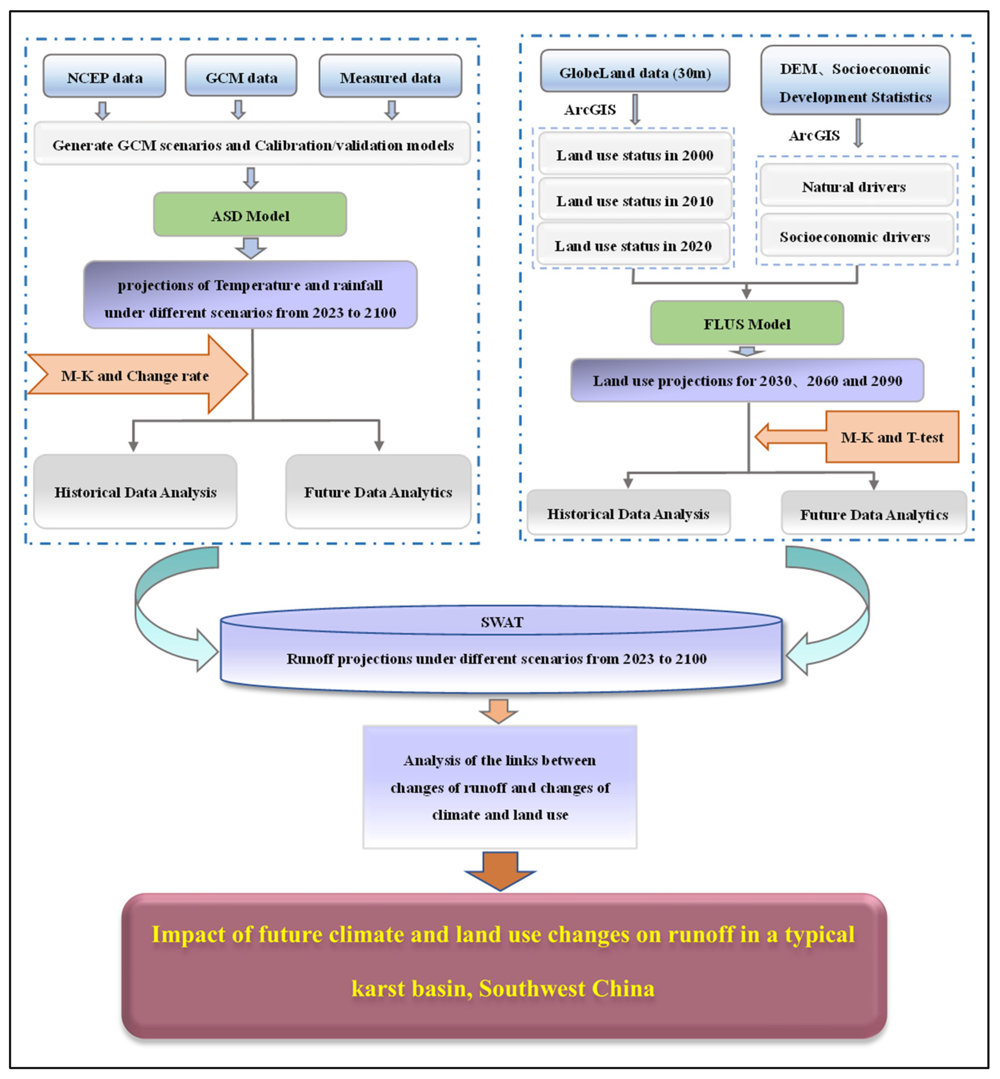
Daily precipitation data were recorded by nine precipitation stations and three hydrological stations: Donghe station (DHS), Linyun station (LYS), Xiajia station (XJS), Jiefu station (JFS), Haokun station (HKS), Chaoli station (CLS), Nongtang station (NTS), Xiatang station (XTS), Pingtang station (PTS), Linhe station (LHS), Bashou station (BSS) and Bailian station (BLS). Daily runoff data were provided by three stations: XJS, PTS and BSS. Meteorological data include daily maximum/minimum temperature, wind speed, relative humidity, solar radiation P data and CanESM5 climate model data in CMIP6 (https://esgf-node.llnl.gov (accessed on 24 September 2021)). Daily precipitation and daily maximum/minimum temperatures for the SSPs1-2.6 scenario (sustainable development road, influenced by a combination of low social vulnerability and low levels of coercion), SSPs2-4.5 scenario (moderate road, influenced by moderate social vulnerability and moderate levels of imposition), and SSPs5-8.5 scenario (fossil-fueled development road, influenced by a combination of high social vulnerability and high levels of forcing) from 2023 to 2100 were obtained by downscaling the NCEP data and CanESM5 climate model data in CMIP6 (https://esgf-node.llnl.gov (accessed on 26 October 2021)). The digital elevation model (DEM) data with a resolution of 30 m was obtained from the geospatial data cloud of the Chinese Academy of Sciences (https://www.gscloud.cn/ (accessed on 12 December 2021)). The soil data were obtained from the HWSDv1.2 soil library and processed using SPAW software by selecting 3 soil parameters SOL_BD, SOL_AWC and SOL_K. The land-use data was provided by GlobeLand30, a global 30 m surface coverage remote sensing data product (http://www.globallandcover.cm (accessed on 12 December 2021)). The methodological framework of this research was shown in Figure 2.

3. Methodology

3.1. Mann-Kendall Trend Test

Mann-Kendall (M-K) is a non-parametric test method that is based on the correlation rank and order of the time series to determine if there is an increasing or decreasing trend in the data [41]. This method judges the presence of a statistically positive or negative trend of data series based on positive or negative of Z-value. In detail, when the absolute value of Z is greater than or equal to 1.645, 1.96 or 2.576, it means that it passes the significance test with a 90%, 95%, or 99% confidence level, respectively. When the absolute value of Z is greater than or equal to 1.645, 1.96 or 2.576, this is indicated by a “*”, “**” or “***”, respectively.

3.2. Downscaling of Global Climate Model

Meteorological data are important input data for hydrological simulation. In order to obtain more accurate future regional meteorological data, this paper uses the ASD model [14] to statistically downscale the GCM and predict the precipitation and temperature under different future scenarios. The NCEP reanalysis data and GCM data are each compared to the corresponding meteorological simulated values output from the ASD statistical downscaling method.
The simulation accuracy of the ASD is analyzed for the calibration period (1963–1998) and the validation period (1999–2014) using two evaluation metrics (θ and RMSE). The θ and RMSE are calculated using the following equations:
θ = 1 n | Q o , i Q s ¯ |
and
R M S E = 1 n i = 1 n ( Q o , i Q s ) 2 ,
where n is the length of the monthly time series; Q o , i is the observed runoff for i-th day; Q s is the simulated runoff in the research period and Q s ¯ is the average simulated runoff.

3.3. Land Use Change Prediction Model

The FLUS model is a portfolio model used to simulate future land use change [42]. Based on the ANN module of the FLUS model, the training samples of each category are randomly selected to complete the neural network training, and then DEM data, natural data and economic data are input as the driving factors and the distribution of each driving factor through standardization is obtained as the land suitability transfer layer. Next, based on the CA module, the initial land use type data is used as input data, and the Land-Use Harmonization 2 (LUH2) dataset is used to preset the target number of changes in each category under different scenarios, then the domain factors of each category are determined according to the regional geomorphological characteristics and economic development, and restricted areas are set up to simulate and predict the land use types in the study area, based on the actual situation of the basin. Finally, the Kappa coefficient is used to test the spatial consistency of land use. The Kappa coefficient ranges from 0 to 1. Generally, when 0.75 < Kappa ≤ 1, the model’s simulation accuracy is high. The Kappa is calculated with the following equation:
K a p p a = P o P e 1 P e ,
where P o and P e are the observed and expected fractions of LUCC, respectively.

3.4. Hydrological Model

The SWAT model is a typical, basin-scale, distributed dynamic hydrological model [43]. It integrates climate, subsurface and other factors to simulate hydrological processes. The model can simulate the quantity and quality of surface and groundwater in various basins, and has been widely used in hydrological simulations [44,45]. In this paper, surface runoff was calculated by using the SCS curve method [46]; evapotranspiration was obtained by the Penman-Monteith method [47] and the Muskingum method [48] was applied to the channel catchment. Thirteen parameters that best describe the spatial heterogeneity of the study area were preferentially selected, and the model was calibrated by using the SUFI-2 algorithm [49] and a multi-site approach [39]. A multi-site calibration was used to calibrate the model parameters to reduce parameter uncertainties and improve the simulation performance of the hydrological model in karst basins [50,51].
The accuracy of the model was quantified using NSE and R 2 as suggested by Ghoraba [52] and Moriasi et al. [53]:
N S E = 1 i = 1 n ( Q o , i Q s , i ) i 2 i = 1 n ( Q o , i Q ¯ o ) 2
and
R 2 = [ i = 1 n ( Q o , i Q ¯ o ) ( Q s , i Q ¯ s ) ] 2 i = 1 n ( Q o , i Q ¯ o ) 2 i = 1 n ( Q s , i Q ¯ s ) 2 ,
where n is the length of the monthly time series; Q o , i is the observed runoff for i-th day; Q s , i is the simulated runoff for i-th day; Q 0 ¯ and Q s ¯ are the average observed and simulated runoff.

4. Results

4.1. Prediction of Climate Factors

4.1.1. Historical Trend Analysis

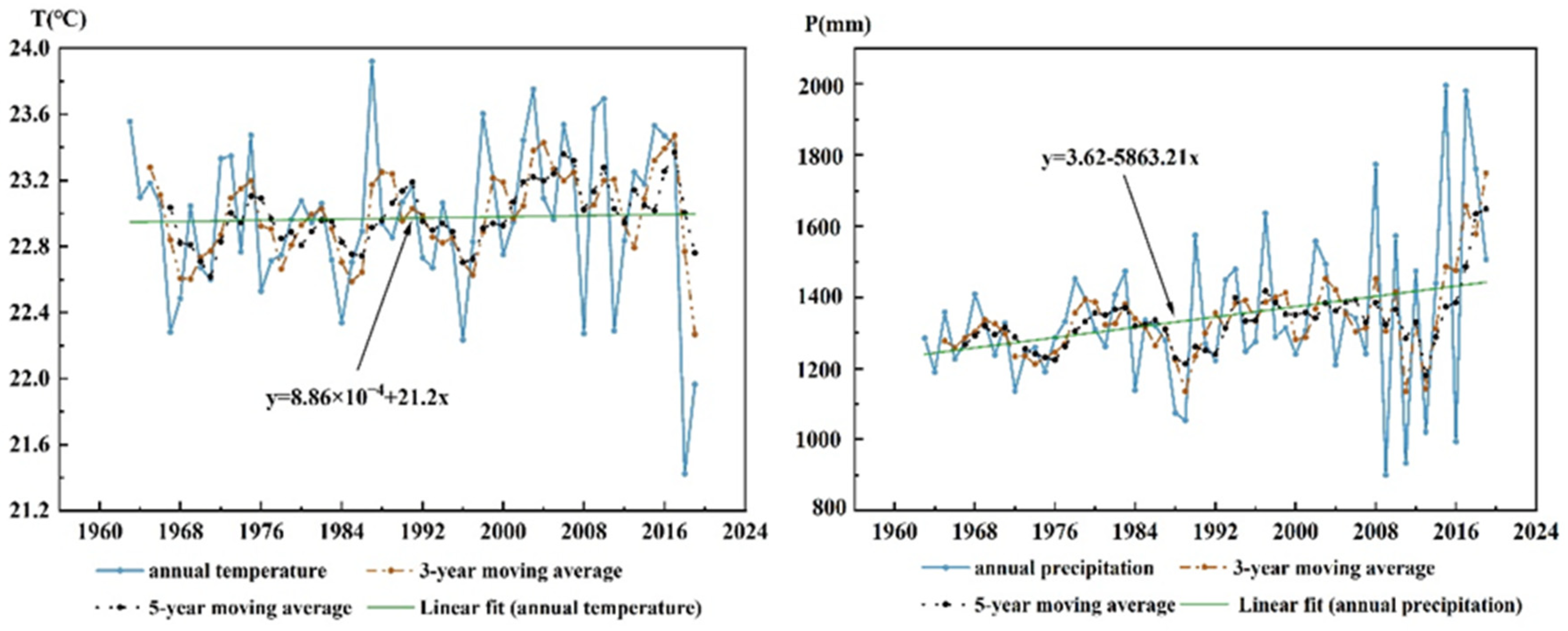
Figure 3 shows the annual precipitation and temperature trend changes from 1963–2019. In terms of precipitation, there was a fluctuating trend with varying rules before 2008, while there was an overall upward trend change after 2008. There was an insignificant upward trend (Z = 1.19) in temperature during 1963–2019. Table 1 shows the statistics of historical annual precipitation and temperature. The multi-year average precipitation was 1341.20 (remark valid for the whole paper), and the multi-year average maximum and minimum temperatures were 27.40 °C and 18.54 °C, respectively. The Z-value of precipitation was 1.93, implying a significant increasing trend of annual average precipitation from 1963–2019. The Z-values of Tmax and Tmin were −0.72 and 4.23, respectively, indicating a slight decrease in maximum temperatures and a significant increasing trend (Z = 4.23 ***) in minimum temperatures during the historical period (1963–2019). Figure 4 shows the variation characteristics of precipitation and temperature.
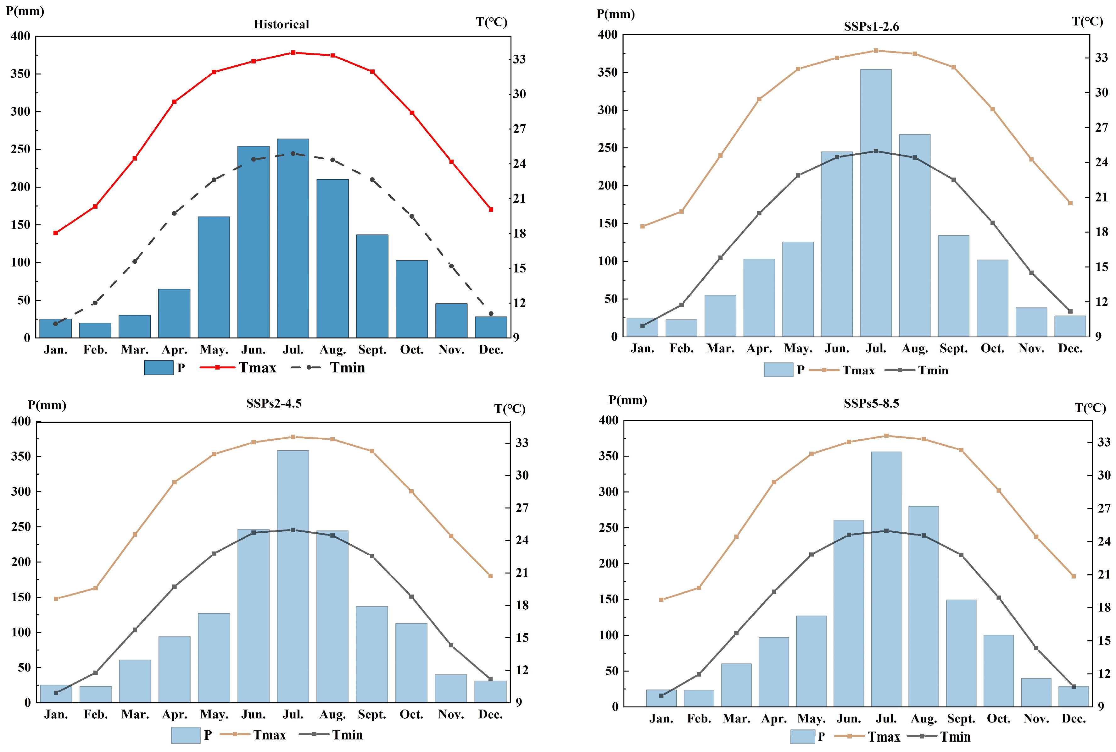
The seasonal variation of precipitation is large, with more precipitation in summer and autumn (May to September) and less precipitation in spring and winter (October to April). The changes in temperature and precipitation have similar characteristics, with the highest temperatures occurring in June or July and the lowest temperatures in January or February. The variations in temperature and precipitation have similar characteristics, with the highest temperatures occurring in summer and the lowest temperatures in winter or spring.

4.1.2. Projection of Precipitation and Temperature

In the calibration period (1963~1998), the average deviation θ of NCEP for the monthly average daily precipitation data is controlled from 0.06 to 0.22 and RMSE from 0.08 to 0.38; the average deviation θ of GCM data (CanESM5 mode) is controlled from 0.22 to 1.32 and RMSE from 0.37 to 1.70. For temperature, daily average maximum/minimum temperature mean and standard deviation (Stcd)with θ and RMSE are less than 0.01, and the simulation is very good. During the validation period (1999~2014), the average deviation θ of NCEP for the monthly average daily precipitation data is controlled from 0.35 to 0.92 and RMSE from 0.44 to 1.20; the average deviation θ of GCM data (CanESM5 model) is controlled from 0.50 to 1.22 and RMSE from 0.88 to 1.80. For temperature, the daily maximum/minimum air temperature mean value in the validation period is slightly less than the accuracy of the calibration period (the daily maximum/minimum temperature standard deviation (Stcd) with θ and RMSE less than 0.229), but also within the accuracy index of good simulation.
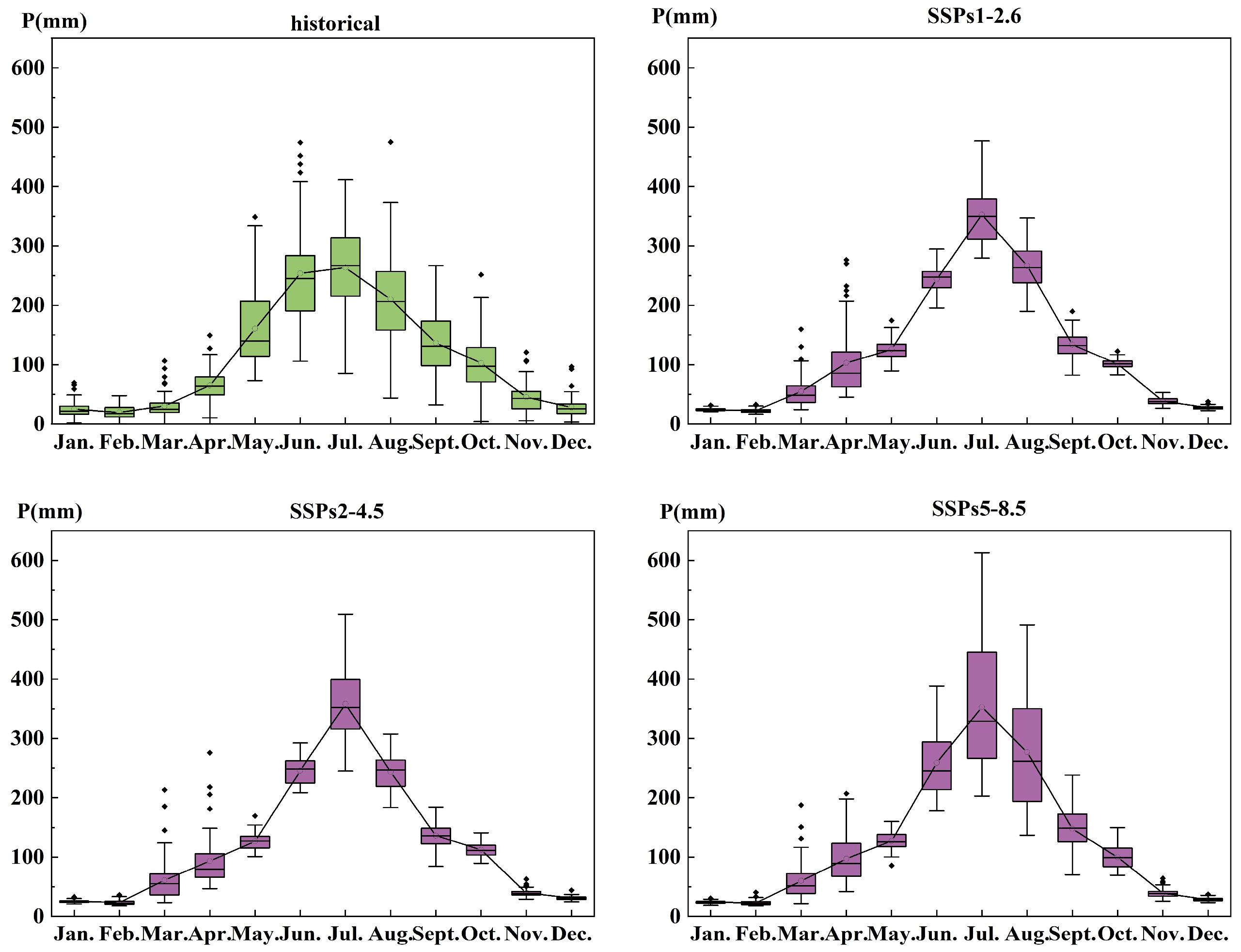
The annual precipitation and temperature in the three scenarios have significant upward trends (Figure 5); the upward trend of SSP5-8.5 is the most obvious (Z = 10.89 ***). The future annual average precipitation will be in the range of 1495.78 mm to 1534.67 mm, representing an increase of 11.53–14.43% compared to the historical average (1341.20 mm). The annual average temperature in the three scenarios suggest increasing trends (Figure 5), with the most pronounced increase in SSP5-8.5 (Z = 6.10 ***). The average annual temperature under different scenarios ranged from 22.98 °C to 23.01 °C, increasing by 0.02–0.15% compared to the historical average (22.97 °C). The increase of average annual precipitation exacerbates the increase of future runoff, further increasing the probability of future flooding. Intuitively, higher temperature should result in higher evaporation, resulting in more evaporation and lower runoff. However, a smaller increase in temperature (0.02–0.15%) may not be effective in reducing the increase in runoff from increased precipitation (11.53–14.43%). As shown in Table 2 and Figure 6, future precipitation increases during the flood season, and rarely increases or decreases during the dry season, which leads to a more uneven intra-annual distribution of precipitation. The shape of the precipitation histogram for the three scenarios is approximately the same as the historical distribution, with the peak occurring in July. However, the July precipitation under the SSPs1-2.6, SSPs2-4.5 and SSPs5-8.5 scenarios increased by 34.2%, 36.0% and 35.0%, respectively, compared to history, which increases the probability of flooding in July. The temperature prediction results under different scenarios had higher consistency. The changes in Tmin were completely unlike those in Tmax, with the minimum temperature increasing and the maximum temperature decreasing for all three climate scenarios (Table 3).

4.2. Prediction of Land Use Change

4.2.1. Historical Land Use

According to the average land use area in 2000, 2010 and 2020, the major land use type was forest and cropland, which accounts for 75.12% and 12.23%, respectively (Table 4). The average proportions of the area of water and artificial surface were both less than 2%. However, the changing trends of these two land use types during the historical period were quite different. The water area was fluctuating, while the artificial surface area was rapidly increasing. At the same time, the area of forest land decreased, grassland increased, and cultivated land fluctuated. The results of the land use transfer matrix calculations (see Supplementary Tables S1 and S2) showed that forests were converted to cropland and grassland in the period 2000–2010. During 2010–2020, cropland was converted to forest land, forest land was converted to grassland and cropland and forest and grassland were converted to impervious area.

4.2.2. Future Land Use

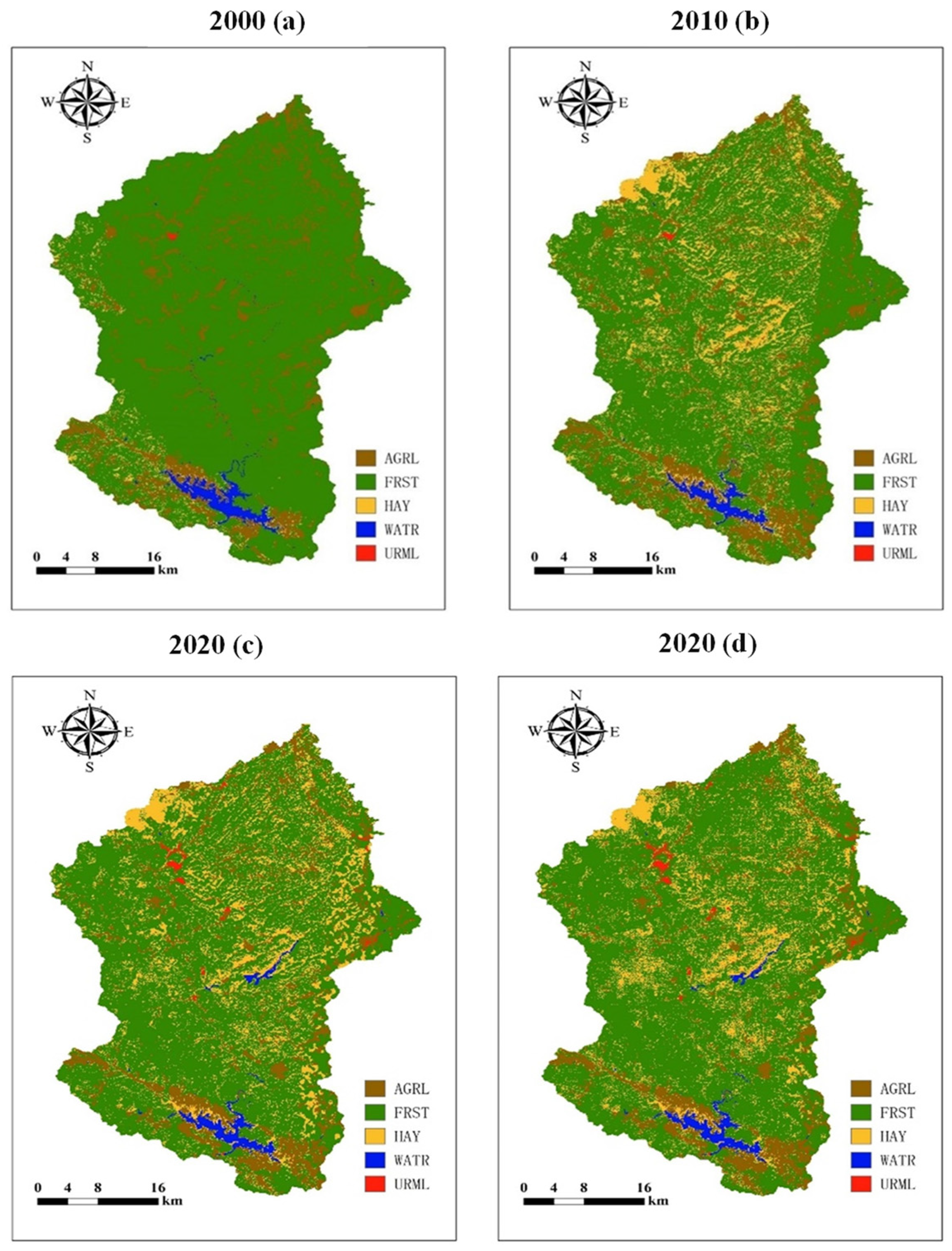
To assess the reliability of the FLUS model, we compared the predicted 2020 land use scenario with the actual land use (Figure 7). It can be seen that the predicted results show spatial characteristics similar to the actual results. In addition, the calculated Kappa coefficient value is 0.78, and the overall accuracy is 0.89. In general, the constructed FLUS model presents good prediction results and can be applied to predict future land spatial patterns under different scenarios.
From the calculation of the transfer matrix (Supplementary Tables S3–S5), under the SSPs1-2.6 scenario, most of the increase in grassland area in 2020–2030 is mainly converted from cropland; in 2060 the area of grassland plummets to zero and is mainly converted to cropland and forest; in 2090 the sudden increase in artificial surface is mainly converted from forest and the area of cropland is mainly converted from forest. Under the SSPs2-4.5 scenario, the increased area of grassland in 2020–2030 is mainly from cropland and forest; the increased area of artificial surface in 2030–2060 is mainly from grassland. Under the SSPs5-8.5 scenario, the area of grassland and artificial surface grows fastest in 2020–2030, mainly from forest land. In general, under the SSPs1-2.6 scenario, a large amount of cropland will be converted to grassland in 2020–2030, grassland will be converted to cropland and forest land in 2060, forest land will be converted to cropland in 2090, and artificial surface will be converted to forest land; under the SSPs2-4.5 scenario, grassland, cropland and artificial surface will be converted in a balanced-cyclic manner; under the SSPs5-8.5 scenario, changes will be mainly concentrated in 2020–2060, and a large amount of forest land will be converted to grassland and artificial surface.

4.3. Hydrological Responses

4.3.1. Calibration and Validation of the SWAT Model

The sequential uncertainty fitting procedure (SUFI-2 algorithm) performed by SWAT-CUP software was used for parameter calibration and uncertainty analysis. Parameter uncertainty was measured by P (the proportion of the measured sequence length in 95 PPU) and r (the mean width divided by the standard deviation of the observed data). First, a large parameter variation space is assumed. Then, the uncertainty range is gradually reduced while monitoring the changes in P and r. The sensitivity matrix and covariance matrix are recalculated each time the parameter range is changed. Finally, the parameters are updated and the next step is performed to bring the simulated values closer to the measured values. Thirteen parameters were selected to characterize the spatial heterogeneity of the study area, and the results of the monthly and daily SWAT model parameters are shown in Supplementary Tables S6 and S7, respectively.
The SWAT model was calibrated using 2003–2006 data, and validated using 2007–2020 data. The model achieved the simulation of daily runoff and monthly runoff, and the simulation results were generally in high agreement with the measured results (see Supplementary Figures S1 and S2). As can be seen in Table 5, in comparison to other stations, the accuracy of the simulation results using XJS data are slightly lower (R2 reaches above 0.8 in the daily runoff simulation except for the XJS (0.71), R2 reaches above 0.9 in the monthly runoff simulation except for the XJS (0.81)), which may be due to the fact that it is located in a karst area with very complex hydrological processes. In general, the SWAT model has high hydrological simulation ( N S E ¯ = 0.83, R 2 ¯ = 0.915) accuracy and is applicable for CbR basin.

4.3.2. Future Runoff Response

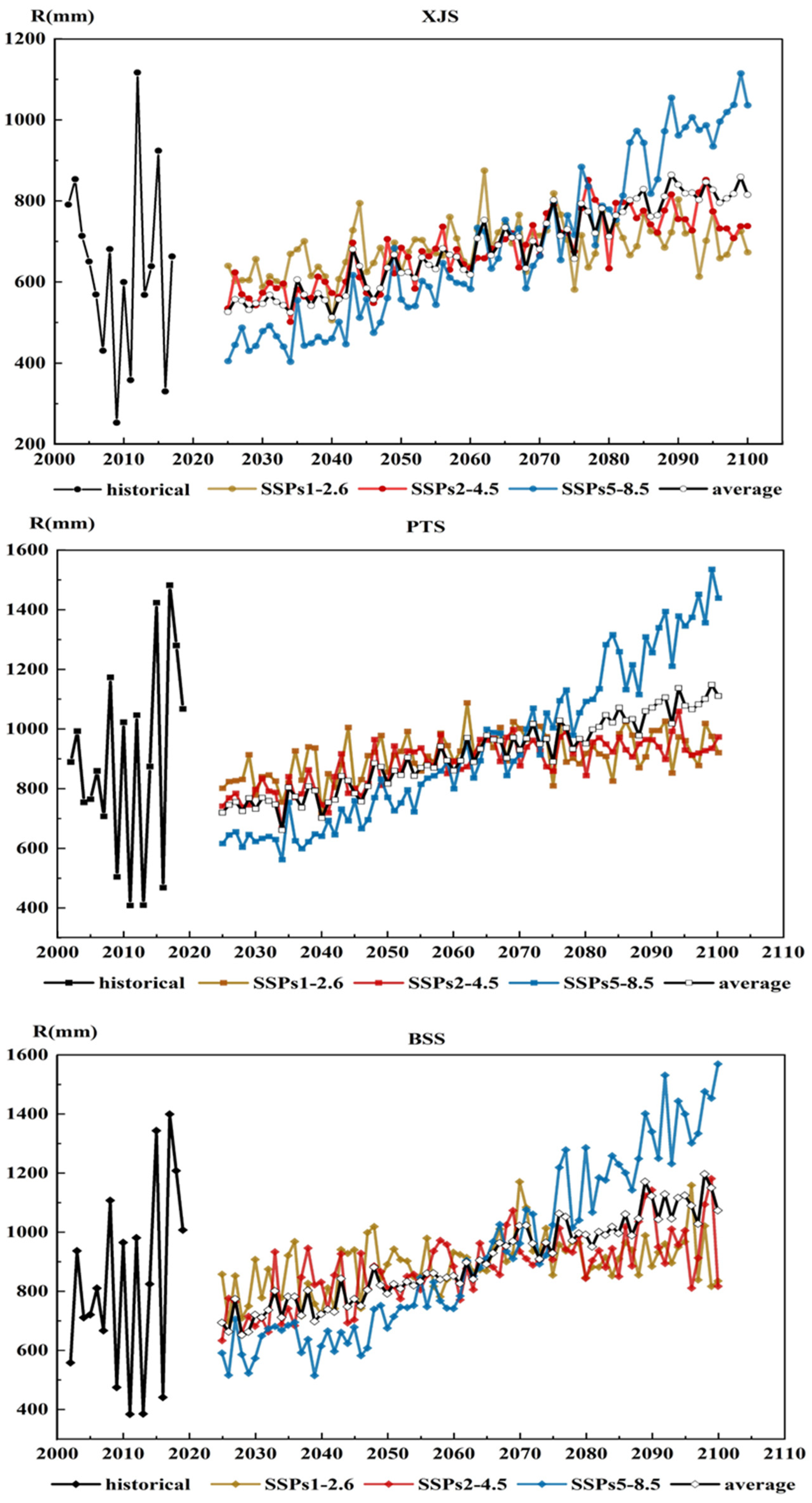
The future land use (2030, 2060, and 2090) as well as future daily precipitation and temperature (2023–2100) were input into SWAT, and future runoff under different scenarios was simulated. Table 6 showed statistics of annual runoff under different future scenarios. The M-K test showed a significant upward trend in future annual runoff (Z > 2.576); the t-test showed there was a significant difference between the simulated future runoff and historical mean (p < 0.05). Compared with the historical mean annual runoff, the simulated mean annual runoff increased under different climate scenarios, and the upward trend is clear (Figure 8).
The differences between the monthly runoff ratios of the three stations in the future period (2025–2100) and the historical period (1963–2019) are shown in Table 7. As can be seen from Table 7, runoff in April is the most sensitive and will increase by 104.35–140.40% compared to the baseline period value (424.34 m3/s), while runoff in July is the least sensitive, with a rate of change between −0.46% and −0.27% of the baseline (4552.03 m3/s).
The runoff box plots (Figure 9) show that the variability and uncertainty of runoff before the main-flood season (June to August) under the three future scenarios are greater than historical, and more frequent and severe flood disasters may occur in the spring. In addition, the bimodal structure of future runoff processes may increase the number of future floods. Under the SSPs5-8.5 scenario, the peak flow in July may continue into August, increasing the probability and duration of floods. Overall, future runoff in the basin is likely to continue to increase, especially during the pre-flood period (April to May). This phenomenon will further exacerbate flood control pressure during the flood season (April to October) and is not conducive to future water management in the basin.
Table 8 shows the differences between the seasonal runoff proportions in the future period (2025–2100) and the historical period (1963–2019). Compared to the historical period, the runoff proportion of XJS and PTS in spring and summer have a decreasing trend, with increases in autumn and winter. The runoff proportion of BSS in summer has a decreasing trend, and increases in spring, autumn and winter. In summary, the three hydrological stations have the same trend in summer, autumn and winter; the proportion of spring runoff is increasing only in BSS. As can be seen from Figure 10, compared to the historical period, runoff proportions of spring (7.73–8.11%), autumn (46.22–47.25%), and winter (13.52–14.8%) will show an increasing trend under three scenarios, while the runoff proportion of summer (30.87–31.50%) will show a decreasing trend. Overall, these changes will result in a more even intra-annual distribution of water resources.

5. Discussion

5.1. Impact of Different Discharge Scenarios and LUCC on Runoff

According to the simulation results, runoff has an increasing trend in its interannual distribution (Figure 8), as well as an uneven seasonal distribution (Figure 10). The above analysis reveals that the average annual temperature, average annual precipitation and average annual runoff will show an increasing trend under different future scenarios. At the annual scale, the increase in precipitation determines the increase in runoff, which is consistent with the conclusions of Wang et al. [54] and Wu et al. [55].
There is more uncertainty on the seasonal scale. In spring, when precipitation increases significantly, the simulated spring runoff will increase, which is the same phenomenon as the overall annual runoff. However, precipitation and temperature will increase and runoff will decrease in summer. Then, precipitation will decrease, but temperature and runoff will increase in winter. Carbonate fractures and crevices in karst areas have high water storage and infiltration rates. Under normal conditions, most of the precipitation infiltrates into the subsurface system of karst areas and usually generates little or no surface runoff; when extreme precipitation events occur, surface karst zone may be temporarily saturated and generate large amounts of runoff [36]. As can be seen in Figure 10, summer runoff in the basin will decrease in the future, possibly due to the small percentage increase in summer precipitation (the increase can be considered as an additional normal precipitation event), which is not sufficient to generate significant runoff in the karst basin. Furthermore, the impact of temperature-increased evaporation may outweigh the impact of precipitation-increased runoff, which may also be a reason for the non-negligible decrease in summer runoff. In the future, the increase in the area of weakly permeable or even impermeable surfaces due to the expansion of urbanization and the reduction of vegetation in winter may have a stronger hindering effect on rainwater infiltration, which may be the direct cause of the increase in winter runoff.

5.2. Discussion on Tmax Decrease and Damped Runoff

In this study, we combined a FLUS model, ASD model, SWAT and multi-site calibration strategy to assess future runoff under climate change and human activities in a karst basin, and found some interesting phenomena, discussed in detail below.
  • In the three future scenarios, Tmax will show a slight downward trend.
It should be noted that the slight downward trend of Tmax in this paper is not contradictory to global warming. The increase in greenhouse gas concentrations forcing temperature rise is global, but other factors such as natural factors, local feedback and regional variations in atmospheric and oceanic circulation can enhance this effect in some regions while weakening it in others. Furthermore, there is some uncertainty in the temperature predictions from the ASD model. As the temperature data we entered were provided by the Baise site in Guangxi, there is some uncertainty in this single site’s ability to represent historical temperature values throughout our study area. Finally, haze has an inhibitory effect on high temperatures. When the haze concentration increases, it is able to reflect the ultraviolet light from the air causing the ground temperature to decrease. In summary, there are many potential reasons for the existence of a decreasing trend in maximum temperatures, such as latitude, topography, atmospheric and oceanic circulation and haze.
2.
There is a difference in runoff variability between the historical and simulated periods.
In the future scenario runoff simulations, the model does not yet adequately capture the monsoon-driven variability of precipitation and associated runoff. Analysis of the simulated and measured results of daily and monthly runoff (see Supplementary Figures S1 and S2) shows that the model is indeed not very good at simulating the extremes, and the simulated extremes of future runoff may be smaller than the actual values. Undeniably, the model has some shortcomings in capturing the characteristics of karst basins. From previous studies [56,57,58], it is known that using multi-site to calibrate and validate model will gain more reasonable results than a single site. As described by Mo et al. [39], for karst with heterogeneous physical properties and irregular and complex flow regimes, multi-site calibrated hydrological models may obtain better simulation results during calibration or validation. On monthly and daily scales, the lowest NSE value is 0.681 and highest is 0.900 for the single-site method, and the lowest NSE value is 0.743 and highest is 0.953 for the multi-site method. Therefore, we used the multi-site method to calibrate and validate the model. The main purpose of this study is to simulate future overall runoff and provide some theoretical basis for ecological protection of the basin and optimization of water resources management, thus, the requirements for the extreme values may not have been sufficiently restrictive. It is certain that the simulation of extreme values will become a difficult and important point for future study. We will also work on improving the model in future studies to make it more applicable to karst zone basins.
Comparing the precipitation box plots (Figure 11) and the runoff box plots (Figure 9), it can be seen that the monthly distribution characteristics of precipitation have some similarity with runoff, especially for the low (SSPs1-2.6) and medium (SSPs2-4.5) discharge scenarios. Precipitation may be an important reason for the generation of runoff damping. The precipitation box plots (Figure 11) shows that the monthly precipitation variability decreases in the SSPs1-2.6 and SSPs2-4.5 scenarios, compared to the historical period. Meanwhile, the monthly runoff variability decreases in the SSPs1-2.6 and SSPs2-4.5 scenarios. It is worth noting that this link between precipitation and runoff seems to be weakened in the high emission scenario (SSPs5-8.5), where monthly precipitation variability increases while monthly runoff variability decreases. The reason for this phenomenon may be that the land use and temperature of the high emission scenario (SSPs5-8.5) also affect damped runoff.
3.
Future research
In future work, we could use the Monte Carlo method to randomly add precipitation variability deviations to the precipitation patterns of the three future scenarios using the characteristic values of the statistical parameters of historical precipitation to produce more realistic runoff variability. Furthermore, we could also use the ensemble Kalman filter to process historical precipitation and intentionally add to the precipitation patterns of the three future scenarios to obtain more realistic runoff variability. Finally, a more accurate prediction of runoff extremes should be generated for the analysis of the severity of future societal impacts.

5.3. Uncertainty Analysis and Future Research

The selection of climate models, simulation models for land use change, and hydrological models, as well as the calibration and validation process of these model parameters, may create uncertainty in the results. Different GCMs can bring different variability characteristics in different study areas. Compared to the CMIP5 model, CMIP6 adds a new concept of shared socioeconomic routes, improves the ability to simulate the current regional temperature and precipitation in China [59], and has been applied by more scholars to the study of the future climate of China [18,60,61]. However, we only selected three emission scenarios from the CMIP6 model in an attempt to provide a range of precipitation and temperature projection data for this study area, which leaves some uncertainty in future climate simulation results. In addition, the construction of hydraulic structures or facilities may destroy the consistency of hydrological data, and generate uncertainty in the model calibration and validation process.

6. Conclusions

To analyze the response of runoff to future climate change and land use changes in the basin, we constructed a framework for future runoff prediction based on ASD, FLUS and SWAT models, and investigated the spatial and temporal characteristics of future precipitation, temperature and land use and assessed their effects on future runoff. Our study’s findings suggest four overarching points. First, the SWAT model based on multi-site calibration have good performance and possess good accuracy in future climate prediction as well as future runoff simulation. Second, throughout the future period, the average temperature will increase by 0.02–0.15% and the average annual precipitation will increase by 11.53–14.43%. Third, responses vary across emission scenarios. Under the SSPs1-2.6 scenario, there is mainly interconversion between cropland and grassland. Under the SSPs2-4.5 scenario, there is an equilibrium-cyclic conversion of grassland, cropland and artificial surface. Under the SSPs5-8.5 scenario, there is a large conversion of forest land to grassland and artificial surface from 2020 to 2060, and little change in all types of land by 2090. Fourth, the future annual runoff will show a significant upward trend, with monthly runoff concentrated in July (peak), August and September. The box plots reflect the increased variability and uncertainty of runoff before the main flood period (June–August) compared to historical runoff, with spring runoff showing more anomalously large values and the potential for more frequent and severe flood hazards. In addition, the future runoff processes will show a bimodal form, which may increase the number of floods occurring in the future. Monsoon precipitation is an important factor affecting future runoff changes. Under the SSPs5-8.5 scenario, there is no significant downward trend in the July peak through August, which may result in a backward shift in the total runoff peak and increase the probability and duration of flooding. The effects of land use and temperature on runoff simulation should not be neglected in the SSPs5-8.5 scenario. The results of the study can provide a reference for water resources allocation and land use management in the CbR Basin.

Supplementary Materials

The following supporting information can be downloaded at: https://www.mdpi.com/article/10.3390/w15122240/s1. Table S1: Area transfer matrix of land use types in Chengbi River Basin from 2000 to 2010, Table S2: Area transfer matrix of land use types in Chengbi River Basin from 2010 to 2020, Table S3: Area transfer matrix of land use types in Chengbi River Basin from 2020 to 2030, Table S4: Area transfer matrix of land use types in Chengbi River Basin from 2030 to 2060, Table S5: Area transfer matrix of land use types in Chengbi River Basin from 2060 to 2090, Table S6: Monthly calibration results of SWAT model parameters, Table S7: Daily calibration results of SWAT model parameters, Figure S1: Results of multi-site monthly runoff simulations for calibration and validation periods, Figure S2: Results of multi-site daily runoff simulations for calibration and validation periods.

Author Contributions

Data curation, Resources, Writing—original draft, C.M.; Conceptualization, Methodology, Writing—original draft, M.B.; Software, Supervision, Writing—reviewing and editing, S.L.; Writing—reviewing and editing, J.D.; Validation, P.T.; Supervision, Z.X.; Investigation, G.T.; Investigation, L.L. All authors have read and agreed to the published version of the manuscript.

Funding

This study was supported by the National Natural Science Foundation of China (Grant Nos. 52269002, 51969004), the Science and Technology Award Incubation Project of Guangxi University (Grant No. 2022BZJL023), and the Guangxi Water Resource Technology Promotion Foundation (SK2021-3-23).

Data Availability Statement

Data cannot be made publicly available; readers should contact the corresponding author for details.

Conflicts of Interest

The authors declare no conflict of interest.

References

  1. Intergovernmental Panel on Climate Change (IPCC). Climate Change 2014: Mitigation of Climate Change: Working Group III Contribution to the Fifth Assessment Report of the Intergovernmental Panel on Climate Change; Cambridge University Press: Cambridge, UK, 2014. [Google Scholar]
  2. Alifu, H.; Hirabayashi, Y.; Imada, Y.; Shiogama, H. Enhancement of river flooding due to global warming. Sci. Rep. 2022, 12, 20687. [Google Scholar] [CrossRef]
  3. Li, Z.L.; Li, W.; Li, Z.J.; Lv, X.Y. Responses of Runoff and Its Extremes to Climate Change in the Upper Catchment of the Heihe River Basin, China. Atmosphere 2023, 14, 539. [Google Scholar] [CrossRef]
  4. Xue, D.X.; Zhou, J.J.; Zhao, X.; Liu, C.F.; Wei, W.; Yang, X.M.; Li, Q.Q.; Zhao, Y.R. Impacts of climate change and human activities on runoff change in a typical arid watershed, NW China. Ecol. Indic. 2021, 121, 107013. [Google Scholar] [CrossRef]
  5. Luo, Y.Y.; Yang, Y.T.; Yang, D.W.; Zhang, S.L. Quantifying the impact of vegetation changes on global terrestrial runoff using the Budyko framework. J. Hydrol. 2020, 590, 125389. [Google Scholar] [CrossRef]
  6. Cheng, G.W.; Liu, Y.; Chen, Y.; Gao, W. Spatiotemporal variation and hotspots of climate change in the Yangtze River Watershed during 1958–2017. J. Geogr. Sci. 2022, 32, 141–155. [Google Scholar] [CrossRef]
  7. Zhou, T.J.; Zou, L.W.; Chen, X.L. Review of the Sixth International Coupling Model Comparison Program (CMIP6). Clim. Chang. Res. 2019, 15, 445–456. (In Chinese) [Google Scholar]
  8. Song, Y.H.; Chung, E.-S.; Shahid, S. Spatiotemporal differences and uncertainties in projections of precipitation and temperature in South Korea from CMIP6 and CMIP5 general circulation models. Int. J. Climatol. 2021, 41, 5899–5919. [Google Scholar] [CrossRef]
  9. Song, Y.H.; Chung, E.-S.; Shahid, S. Differences in extremes and uncertainties in future runoff simulations using SWAT and LSTM for SSP scenarios. Sci. Total Environ. 2022, 838, 156162. [Google Scholar] [CrossRef] [PubMed]
  10. Chen, C.Z.; Gan, R.; Feng, D.M.; Yang, F.; Zuo, Q.T. Quantifying the contribution of SWAT modeling and CMIP6 inputting to streamflow prediction uncertainty under climate change. J. Clean. Prod. 2022, 364, 132675. [Google Scholar] [CrossRef]
  11. Adachi, S.A.; Tomita, H. Methodology of the Constraint Condition in Dynamical Downscaling for Regional Climate Evaluation: A Review. Atmosphere 2020, 125, e2019JD032166. [Google Scholar] [CrossRef]
  12. Araya-Osses, D.; Casanueva, A.; Román-Figueroa, C.; Uribe, J.M.; Paneque, M. Climate change projections of temperature and precipitation in Chile based on statistical downscaling. Clim. Dyn. 2020, 54, 4309–4330. [Google Scholar] [CrossRef] [Green Version]
  13. Li, X.; Zhang, K.; Babovic, V. Projections of Future Climate Change in Singapore Based on a Multi-site Multivariate Downscaling Approach. Water 2019, 11, 2300. [Google Scholar] [CrossRef] [Green Version]
  14. Hessami, M.; Gachon, P.; Ouarda, T.B.M.J.; St-Hilaire, A. Automated regression-based statistical downscaling tool. Environ. Model. Softw. 2008, 23, 813–834. [Google Scholar] [CrossRef]
  15. Ahmadi-Sani, N.; Razaghnia, L.; Pukkala, T. Effect of Land-Use Change on Runoff in Hyrcania. Land 2022, 11, 220. [Google Scholar] [CrossRef]
  16. Wang, Z.P.; Tian, J.C.; Feng, K.P. Response of runoff towards land use changes in the Yellow River Basin in Ningxia, China. PLoS ONE 2022, 17, e0265931. [Google Scholar] [CrossRef]
  17. Liu, X.P.; Liang, X.; Li, X.; Xu, X.C.; Ou, J.P.; Chen, Y.M.; Li, S.Y.; Wang, S.J.; Pei, F.C. A future land use simulation model (FLUS) for simulating multiple land use scenarios by coupling human and natural effects. Landsc. Urban Plan. 2017, 168, 94–116. [Google Scholar] [CrossRef]
  18. Guan, X.X.; Zhang, J.Y.; Bao, Z.X.; Liu, C.S.; Jin, J.L.; Wang, G.Q. Past variations and future projection of runoff in typical basins in 10 water zones, China. Sci. Total Environ. 2021, 798, 149277. [Google Scholar] [CrossRef] [PubMed]
  19. Perera, T.; McGree, J.M.; Egodawatta, P.; Jinadasa, K.B.S.N.; Goonetilleke, A. A Bayesian approach to model the trends and variability in urban stormwater quality associated with catchment and hydrologic parameters. Water Res. 2021, 197, 117076. [Google Scholar] [CrossRef] [PubMed]
  20. Tongal, H.; Booij, M.J. Simulation and forecasting of streamflows using machine learning models coupled with base flow separation. J. Hydrol. 2018, 564, 266–282. [Google Scholar] [CrossRef]
  21. Wagner, P.D.; Bieger, K.; Arnold, J.G.; Fohrer, N. Representation of hydrological processes in a rural lowland catchment in Northern Germany using SWAT and SWAT+. Hydrol. Process. 2022, 36, e14589. [Google Scholar] [CrossRef]
  22. Shi, L.J.; Feng, P.Y.; Wang, B.; Liu, D.L.; Zhang, H.; Liu, J.D.; Yu, Q. Assessing future runoff changes with different potential evapotranspiration inputs based on multi-model ensemble of CMIP5 projections. J. Hydrol. 2022, 612, 128042. [Google Scholar] [CrossRef]
  23. Li, Z.L.; Li, Q.J.; Wang, J.; Feng, Y.R.; Shao, Q.X. Impacts of projected climate change on runoff in upper reach of Heihe River basin using climate elasticity method and GCMs. Sci. Total Environ. 2020, 716, 137072. [Google Scholar] [CrossRef] [PubMed]
  24. Ji, H.Y.; Peng, D.Z.; Gu, Y.; Luo, X.Y.; Pang, B.; Zhu, Z.F. Snowmelt Runoff in the Yarlung Zangbo River Basin and Runoff Change in the Future. Remote Sens. 2022, 15, 55. [Google Scholar] [CrossRef]
  25. Basu, A.S.; Gill, L.W.; Pilla, F.; Basu, B. Assessment of Variations in Runoff Due to Landcover Changes Using the SWAT Model in an Urban River in Dublin, Ireland. Sustainability 2022, 14, 534. [Google Scholar] [CrossRef]
  26. Arnold, J.G.; Allen, P.M. Automated Methods for Estimating Baseflow and Ground Water Recharge from Streamflow Records. J. Am. Water Resour. Assoc. 1999, 35, 411–424. [Google Scholar] [CrossRef]
  27. Zhu, Q.; Liang, R.; Jin, H.; Wang, X.Z. Runoff simulation in the Arashi River Basin based on SWAT model. Water Resour. Power 2013, 31, 25–27. (In Chinese) [Google Scholar]
  28. Zhang, S.J.; Cao, C.; Wang, Z.Y.; Lan, J.Z.; Tian, W.; Li, X.D.; Huang, T.S. Response of Runoff Yield to Land Use Changes in the Small Watershed of Core Area for 2022 Winter Olympic Games in Zhangjiakou City Based on SWAT Model. Forests 2022, 13, 853. [Google Scholar] [CrossRef]
  29. Sîrodoev, I.; Corobov, R.; Sîrodoev, G.; Trombitsky, I. Modelling Runoff within a Small River Basin under the Changing Climate: A Case Study of Using SWAT in the Bălțata River Basin (The Republic of Moldova). Land 2022, 11, 167. [Google Scholar] [CrossRef]
  30. Yang, C.D.; Xu, M.; Fu, C.S.; Kang, S.C.; Luo, Y. The Coupling of Glacier Melt Module in SWAT+ Model Based on Multi-Source Remote Sensing Data: A Case Study in the Upper Yarkant River Basin. Remote Sens. 2022, 14, 6080. [Google Scholar] [CrossRef]
  31. Van Liew, M.W.; Arnold, J.G.; Garbrecht, J.D. Hydrologic Simulation on Agricultural Watersheds: Choosing between Two Models. Trans. ASAE 2003, 46, 1539–1551. [Google Scholar] [CrossRef]
  32. Wu, J.K.; Li, H.Y.; Zhou, J.X.; Tai, S.Y.; Wang, X.L. Variation of Runoff and Runoff Components of the Upper Shule River in the Northeastern Qinghai-Tibet Plateau under Climate Change. Water 2021, 13, 3357. [Google Scholar] [CrossRef]
  33. Kalugin, A. Future Climate-Driven Runoff Change in the Large River Basins in Eastern Siberia and the Far East Using Process-based Hydrological Models. Water 2022, 14, 609. [Google Scholar] [CrossRef]
  34. Tang, Y.Z.; Huo, J.J.; Zhu, D.J.; Yuan, Z. Simulation of the Water Storage Capacity of Siling Co Lake on the Tibetan Plateau and Its Hydrological Response to Climate Change. Water 2022, 14, 3175. [Google Scholar] [CrossRef]
  35. Hartmann, A.; Goldscheider, N.; Wagener, T.; Lange, J.; Weiler, M. Karst water resources in a changing world: Review of hydrological modeling approaches. Rev. Geophys. 2014, 52, 218–242. [Google Scholar] [CrossRef]
  36. Ye, Q.J.; Li, Z.W.; Duan, L.X.; Xu, X.L. Decoupling the influence of vegetation and climate on intra-annual variability in runoff in karst watersheds. Sci. Total Environ. 2022, 824, 153874. [Google Scholar] [CrossRef]
  37. Mo, C.X.; Lai, S.F.; Yang, Q.; Huang, K.K.; Lei, X.B.; Yang, L.F.; Yan, Z.W.; Jiang, C.H. A comprehensive assessment of runoff dynamics in response to climate change and human activities in a typical karst watershed, southwest China. J. Environ. Manag. 2023, 332, 117380. [Google Scholar] [CrossRef] [PubMed]
  38. Mo, C.X.; Ruan, Y.L.; Xiao, X.G.; Lan, H.K.; Jin, J.L. Impact of climate change and human activities on the baseflow in a typical karst basin, Southwest China. Ecol. Indic. 2021, 126, 107628. [Google Scholar] [CrossRef]
  39. Mo, C.X.; Chen, X.R.; Lei, X.B.; Wang, Y.F.; Ruan, Y.L.; Lai, S.F.; Xing, Z.X. Evaluation of Hydrological Simulation in a Karst Basin with Different Calibration Methods and Rainfall InputS. Atmosphere 2022, 13, 844. [Google Scholar] [CrossRef]
  40. Mo, C.X.; Ruan, Y.L.; He, J.Q.; Jin, J.L.; Liu, P.; Sun, G.K. Frequency analysis of precipitation extremes under climate change. Int. J. Climatol. 2019, 39, 1373–1387. [Google Scholar] [CrossRef]
  41. Abebe, S.A.; Qin, T.L.; Zhang, X.; Yan, D.H. Wavelet transform-based trend analysis of streamflow and precipitation in Upper Blue Nile River basin. J. Hydrol. Reg. Stud. 2022, 44, 101251. [Google Scholar] [CrossRef]
  42. Wu, R.; Lan, H.F.; Cao, Y.X.; Li, P.Y. Optimization of low-carbon land use in Chengdu based on multi-objective linear programming and the future land use simulation model. Front. Environ. Sci. 2022, 10, 989747. [Google Scholar] [CrossRef]
  43. Gong, L.; Zhang, X.; Pan, G.Y.; Zhao, J.Y.; Zhao, Y. Hydrological responses to co-impacts of climate change and land use/cover change based on CMIP6 in the Ganjiang River, Poyang Lake basin. Anthropocene 2023, 41, 100368. [Google Scholar] [CrossRef]
  44. Teshager, A.D.; Gassman, P.W.; Secchi, S.; Schoof, J.T.; Misgna, G. Modeling Agricultural Watersheds with the Soil and Water Assessment Tool (SWAT): Calibration and Validation with a Novel Procedure for Spatially Explicit HRUs. Environ. Manag. 2016, 57, 894–911. [Google Scholar] [CrossRef] [Green Version]
  45. Yang, W.T.; Long, D.; Bai, P. Impacts of future land cover and climate changes on runoff in the mostly afforested river basin in North China. J. Hydrol. 2019, 570, 201–219. [Google Scholar] [CrossRef]
  46. US Soil Conservation Service. SCS National Engineering Handbook, Section 4-Hydrology; USDA—Soil Conservation Service: Washington, DC, USA, 1971; Volume 39, pp. 1076–1333.
  47. Alemayehu, T.; Griensven, A.V.; Bauwens, W. Evaluating CFSR and WATCH Data as Input to SWAT for the Estimation of the Potential Evapotranspiration in a Data-Scarce Eastern-African Catchment. J. Hydrol. Eng. 2016, 21, 05015028. [Google Scholar] [CrossRef]
  48. Pati, A.; Sen, S.; Perumal, M. Modified Channel-Routing Scheme for SWAT Model. J. Hydrol. Eng. 2018, 23, 04018019. [Google Scholar] [CrossRef]
  49. Abbaspour, K.C.; Rouholahnejad, E.; Vaghefi, S.; Srinivasan, R.; Yang, H.; Kløve, B. A continental-scale hydrology and water quality model for Europe: Calibration and uncertainty of a high-resolution large-scale SWAT model. J. Hydrol. 2015, 524, 733–752. [Google Scholar] [CrossRef] [Green Version]
  50. Wang, L.; Chen, X.W. Runoff simulation in Jinjiang River Basin based on 3 station calibration and verification. Sci. Soil Water Conserv. China 2007, 6, 21–26. (In Chinese) [Google Scholar] [CrossRef]
  51. Vigiak, O.; Malagó, A.; Bouraoui, F.; Vanmaercke, M.; Poesen, J. Adapting SWAT hillslope erosion model to predict sediment concentrations and yields in large Basins. Sci. Total Environ. 2015, 538, 855–875. [Google Scholar] [CrossRef] [PubMed]
  52. Ghoraba, S.M. Hydrological modeling of the Simly Dam watershed (Pakistan) using GIS and SWAT model. Alex. Eng. J. 2015, 54, 583–594. [Google Scholar] [CrossRef] [Green Version]
  53. Moriasi, D.N.; Arnold, J.G.; Van Liew, M.W.; Bingner, R.L.; Harmel, R.D.; Veith, T.L. Model Evaluation Guidelines for Systematic Quantification of Accuracy in Watershed Simulations. Trans. ASABE. 2007, 50, 885–900. [Google Scholar] [CrossRef]
  54. Wang, R.N.; Peng, W.Q.; Liu, X.B.; Jiang, G.L.; Wu, W.Q.; Chen, X.K. Characteristics of Runoff Variations and Attribution Analysis in the Poyang Lake Basin over the Past 55 Years. Sustainability 2020, 12, 944. [Google Scholar] [CrossRef] [Green Version]
  55. Wu, L.H.; Wang, S.J.; Bai, X.Y.; Chen, F.; Li, C.J.; Ran, C.; Zhang, S.R. Identifying the Multi-Scale Influences of Climate Factors on Runoff Changes in a Typical Karst Watershed Using Wavelet Analysis. Land 2022, 11, 1284. [Google Scholar] [CrossRef]
  56. Bai, J.W.; Shen, Z.Y.; Yan, T.Z. A comparison of single- and multi-site calibration and validation: A case study of SWAT in the Miyun Reservoir watershed, China. Front. Earth Sci. 2017, 11, 592–600. [Google Scholar] [CrossRef]
  57. Nkiaka, E.; Nawaz, N.R.; Lovett, J.C. Effect of single and multi-site calibration techniques on hydrological model performance, parameter estimation and predictive uncertainty: A case study in the Logone catchment, Lake Chad basin. Stoch. Environ. Res. Risk Assess. 2018, 32, 1665–1682. [Google Scholar] [CrossRef] [Green Version]
  58. Wang, S.; Zhang, Z.; Sun, G.; Strauss, P.; Guo, J.; Tang, Y.; Yao, A. Multi-site calibration, validation, and sensitivity analysis of the MIKE SHE Model for a large watershed in northern China. Hydrol. Earth Syst. Sci. 2012, 16, 4621–4632. [Google Scholar] [CrossRef] [Green Version]
  59. Zhu, H.H.; Jiang, Z.H.; Li, L. Projection of climate extremes in China, an incremental exercise from CMIP5 to CMIP6. Sci. Bull. 2021, 66, 2528–2537. [Google Scholar] [CrossRef] [PubMed]
  60. Wang, Y.; Xu, H.M.; Li, Y.H.; Liu, L.L.; Hu, Z.H.; Xiao, C.; Yang, T.T. Climate Change Impacts on Runoff in the Fujiang River Basin Based on CMIP6 and SWAT Model. Water 2022, 14, 3614. [Google Scholar] [CrossRef]
  61. Zhou, J.Y.; Lu, H.; Yang, K.; Jiang, R.J.; Yang, Y.; Wang, W.; Zhang, X.J. Projection of China’s future runoff based on the CMIP6 mid-high warming scenarios. Sci. China Earth Sci. 2023, 66, 528–546. [Google Scholar] [CrossRef]
Figure 1. Location of the CbR basin and distribution of the stations.
Water 15 02240 g001
Figure 2. Research Process Framework.
Water 15 02240 g002
Figure 3. Average annual temperature, average annual precipitation and moving average in 1963–2019 (Data sources are consistent with Table 1).
Water 15 02240 g003
Figure 4. Monthly distribution of multi-year average precipitation and temperature in 1963–2019 (Data sources are consistent with Table 1).
Water 15 02240 g004
Figure 5. Annual precipitation and temperature of three scenarios during 2025–2100.
Water 15 02240 g005
Figure 6. Monthly distribution of precipitation and temperature for historical and future three scenarios.
Water 15 02240 g006
Figure 7. Historical land use (2000 (a), 2010 (b)), actual land use in 2020 (c) and simulated land use 2020 (d).
Water 15 02240 g007
Figure 8. Annual runoff curves for historical and future periods under different scenarios of XJS, PTS and BSS.
Water 15 02240 g008
Figure 9. Box plots of monthly runoff of the BSS during historical and future periods under different scenarios (The BSS is located at the outlet section of the study basin in this paper).
Water 15 02240 g009
Figure 10. Cumulative histograms of precipitation and runoff ratios, ratios of precipitation, temperature and runoff depth change in 2025–2100 (The BSS is located at the outlet section of the study basin in this paper).
Water 15 02240 g010
Figure 11. Box plots of monthly precipitation during historical and future period under different scenarios.
Water 15 02240 g011
Table 1. Statistics of average annual precipitation and temperature in 1963–2019 (Precipitation data are surface rainfall from 12 stations (DHS, LYS, XJS, JFS, HKS, CLS, NTS, XTS, PTS, LHS, BSS and BLS), temperature data are from Baise station).
IndicatorsAverage ValueZ-Value
P1341.201.93 *
Tmax27.40−0.72
Tmin18.544.23 ***
Taverage22.971.19
Table 2. Seasonal distribution of average annual precipitation under three scenarios in 2025–2100 (Spring is from February to April; summer is from May to July; autumn is from August to October; winter is from November to January of the following year).
SeasonalHistorical
(mm)
SSPs1-2.6SSP2-4.5SSP5-8.5
Spring114.94180.55178.26180.29
Summer678.43724.12732.06743.73
Autumn449.47503.32493.95529.48
Winter98.3690.5796.0691.89
Annual1341.201498.571500.331545.39
Table 3. Statistics of temperature for three scenarios in 2025–2100.
Temperature (°C) AverageChange Rate
°C/Decade
Z-Value
SSPs1-2.6Tmax27.52−6.58 × 10⁻³ (close to 0)−0.55
Tmin18.440.052.64 ***
SSPs2-4.5Tmax27.53−8.35 × 10⁻³ (close to 0)−1.10
Tmin18.450.095.34 ***
SSPs5-8.5Tmax27.57−0.04−4.18 ***
Tmin18.460.187.77 ***
Table 4. Area, proportion and change rate of each land type during 2000–2020.
Land Use TypeAverage
Area (km2)
Proportion (%)Amplitude of Variation (km2/a)Change Range (%)
2000–20102010–20202000–20102010–2020
Cropland259.1412.2320.50−15.294.94−4.44
Forest land1591.7375.12−17.64−0.28−31.78−0.42
Grassland232.3110.96791.2612.2027.693.81
Water area32.041.51−23.9710.20−0.890.29
Artificial surface3.760.1828.00603.130.030.77
Table 5. Accuracy evaluation indicators at the daily and monthly scale.
TimeStationMonthly ScaleDaily Scale
NSER2NSER2
Calibration PeriodXJS0.890.940.790.83
PTS0.880.930.840.86
BSS0.820.940.780.84
Validation PeriodXJS0.780.810.690.71
PTS0.850.930.810.84
BSS0.770.940.700.81
Table 6. Statistics of annual runoff for different scenarios in 2025–2100.
StationScenarioAnnual Average Runoff
(108 m3)
Z-Value
(M-K Test)
p-Value
(t-Test)
XJShistorical633.73−0.94
SSPs1-2.6684.624.62 ***0.001
SSPs2-4.5678.868.06 ***0.001
SSPs5-8.5686.7810.46 ***0.024
average683.429.92 ***0.001
PTShistorical860.711.26
SSPs1-2.6912.854.45 ***0.001
SSPs2-4.5885.306.79 ***0.011
SSPs5-8.5933.5911.00 ***0.018
average910.5810.47 ***0.001
BSShistorical794.421.71 *
SSPs1-2.6895.763.79 ***0.001
SSPs2-4.5880.576.44 ***0.001
SSPs5-8.5927.4110.45 ***0.001
average901.2510.48 ***0.001
Table 7. Differences between the proportion of monthly runoff for the future period and the historical period at the three hydrological stations (%).
StationXJSPTSBSS
Month
SSPs1-2.6SSPs2-4.5SSPs5-8.5SSPs1-2.6SSPs2-4.5SSPs5-8.5SSPs1-2.6SSPs2-4.5SSPs5-8.5
Jan.31.0122.2931.9767.2086.1070.0724.7336.9527.05
Feb.−15.94−22.14−16.3512.5727.6611.12−9.231.57−10.83
Mar.−78.56−79.94−78.33−63.12−60.43−62.4268.58100.0094.71
Apr.−89.75−89.04−90.06−80.51−80.46−80.70140.40104.35116.96
May.−86.63−83.10−86.89−86.19−85.97−85.57−57.51−57.49−56.21
Jun.−56.14−50.66−52.05−65.61−67.19−62.51−59.90−60.84−54.37
Jul.11.536.1311.17−14.80−20.42−14.80−1.60−4.60−0.27
Aug.33.5832.9527.9011.641.9915.017.760.9512.45
Sept.92.4290.0595.4778.2370.8083.4561.3157.2068.28
Oct.120.80118.57124.47154.17153.27158.96125.85126.69132.89
Nov.82.5778.9683.03125.76136.02127.1587.2895.4690.42
Dec.98.0889.5397.79145.65162.82146.3593.00106.3998.27
Table 8. Differences between the seasonal runoff proportion in the future and base period of the three hydrological stations (%).
StationScenarioSpringSummerAutumnWinter
XJSSSPs1-2.6−70.76−32.8567.9075.57
SSPs2-4.5−72.18−32.2866.4569.44
SSPs5-8.5−70.90−31.3666.6175.93
PTSSSPs1-2.6−52.14−46.2252.97119.44
SSPs2-4.5−47.56−49.3245.32133.42
SSPs5-8.5−52.36−44.8157.08120.94
BSSSSPs1-2.679.91−33.9542.1775.36
SSPs2-4.577.19−35.6637.3785.87
SSPs5-8.577.81−30.8747.9178.91
Disclaimer/Publisher’s Note: The statements, opinions and data contained in all publications are solely those of the individual author(s) and contributor(s) and not of MDPI and/or the editor(s). MDPI and/or the editor(s) disclaim responsibility for any injury to people or property resulting from any ideas, methods, instructions or products referred to in the content.