


Gaussian Process Regression and Cooperation Search Algorithm for Forecasting Nonstationary Runoff Time Series


Abstract
1. Introduction
2. Methods
2.1. Gaussian Process Regression (GPR)
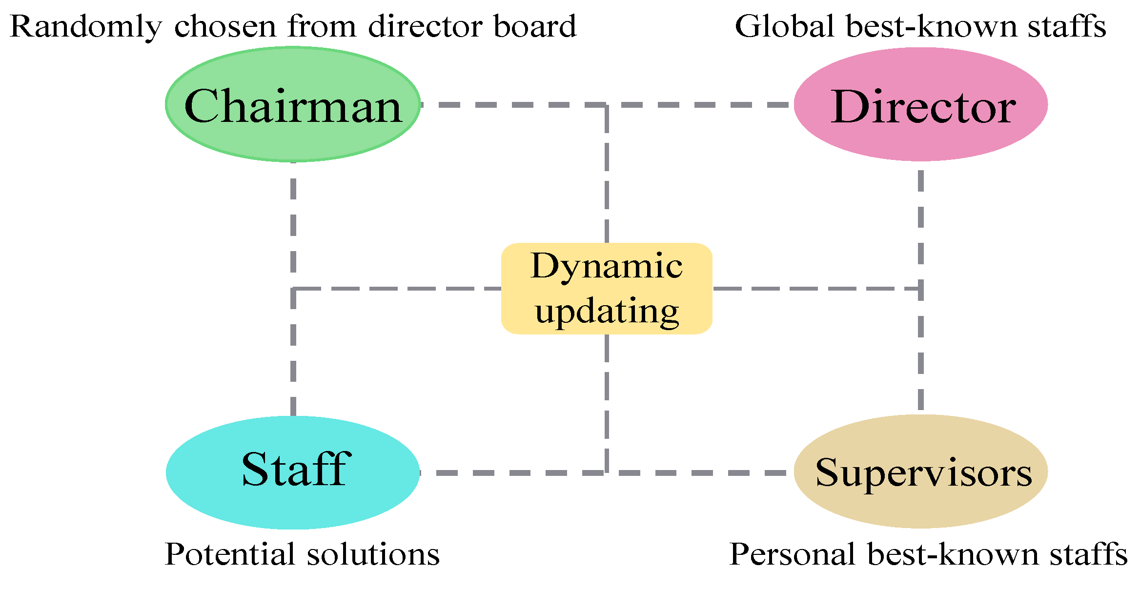
2.2. Cooperation Search Algorithm (CSA)
- (1)
- Team building phase. The initial positions of all staff members in the team are determined by Equation (8). Based on the fitness value, M elite solutions are used to form the exterior leader set.
- (2)
- Team communication operator. Each solution has the opportunity to acquire fresh insights from leader staff members. As showed in Equation (9), the team communication operator uses three components: the expertise A from the chairman, the cumulative knowledge B from the leader staff members in board of directors, and the combined knowledge C from leader staff members in the board of supervisors. The chairman is selected randomly from M global best-known solutions, whereas all directors and supervisors are assigned equal roles. The detailed equations are given as below:
- (3)
- Reflective learning operator. In addition to studying from elite agents, each agent can also acquire new information by considering their own experiences and observations, which can be represented as follows:
- (4)
- Internal competition operator. By guaranteeing retention of the high-quality agents, the competitiveness of the swarm can be gradually enhanced by the following equation:
2.3. Proposed Runoff Forecasting Method
3. Performance Evaluation Criteria
4. Case Studies
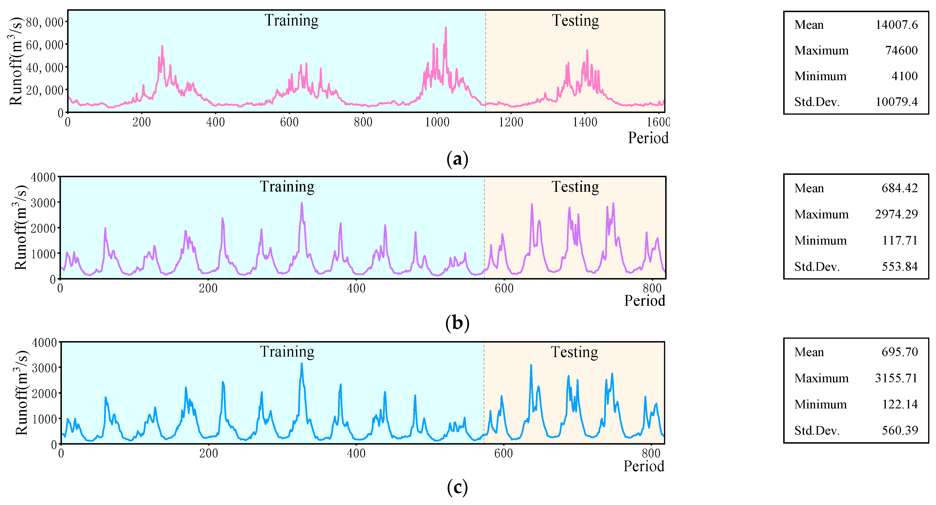
4.1. Engineering Background
4.2. Model Development
4.3. Experiment Results
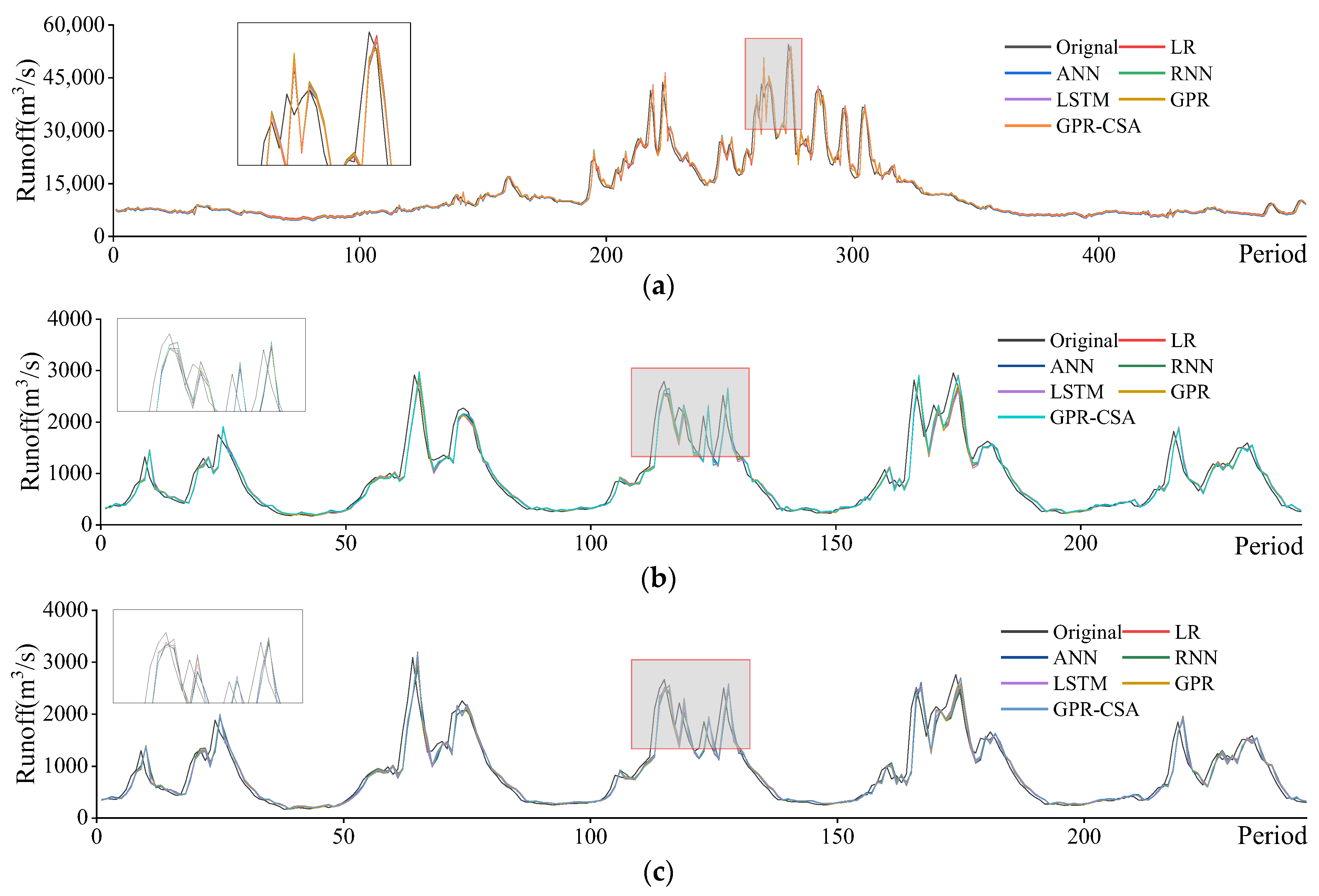
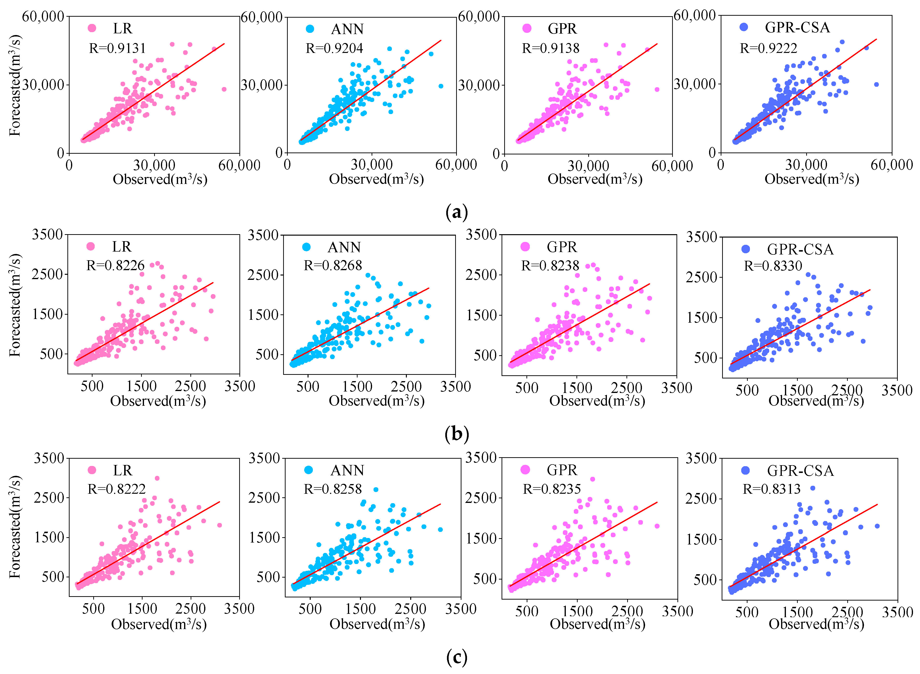
4.3.1. Case 1: One-Step-Ahead Prediction Outcomes
4.3.2. Case 2: Two-Step-Ahead Prediction Outcomes
4.3.3. Case 3: Three-Step-Ahead Prediction Outcomes
4.4. Simulation Discussion
4.4.1. Analysis of the Kernel Function
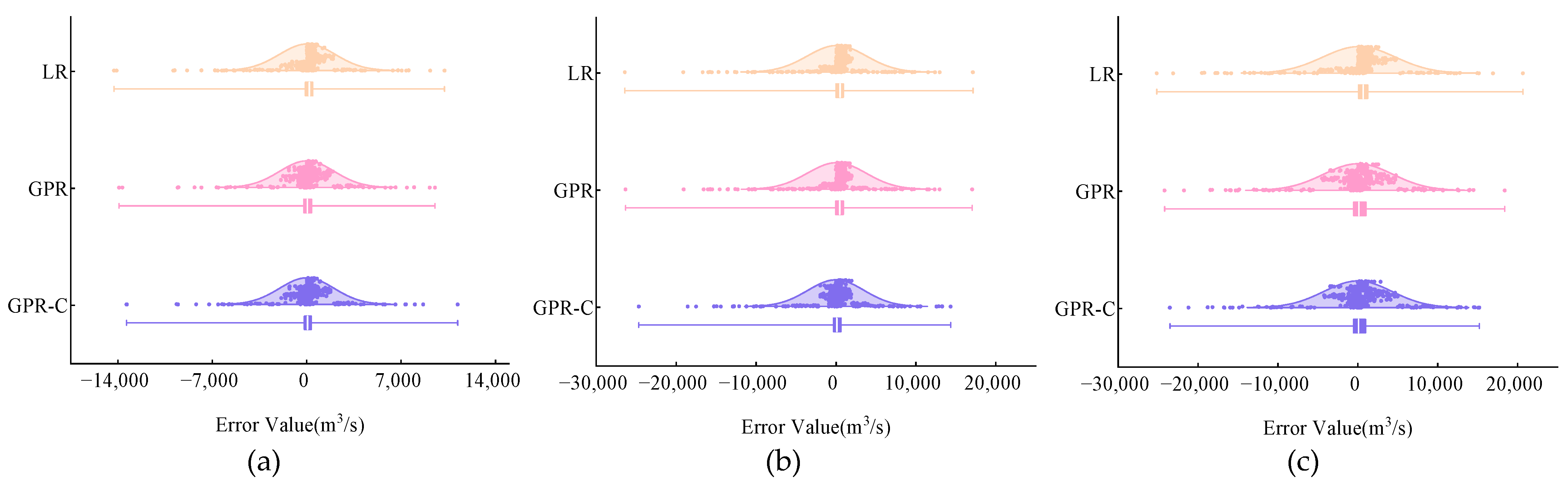
4.4.2. Analysis of the Forecast Errors
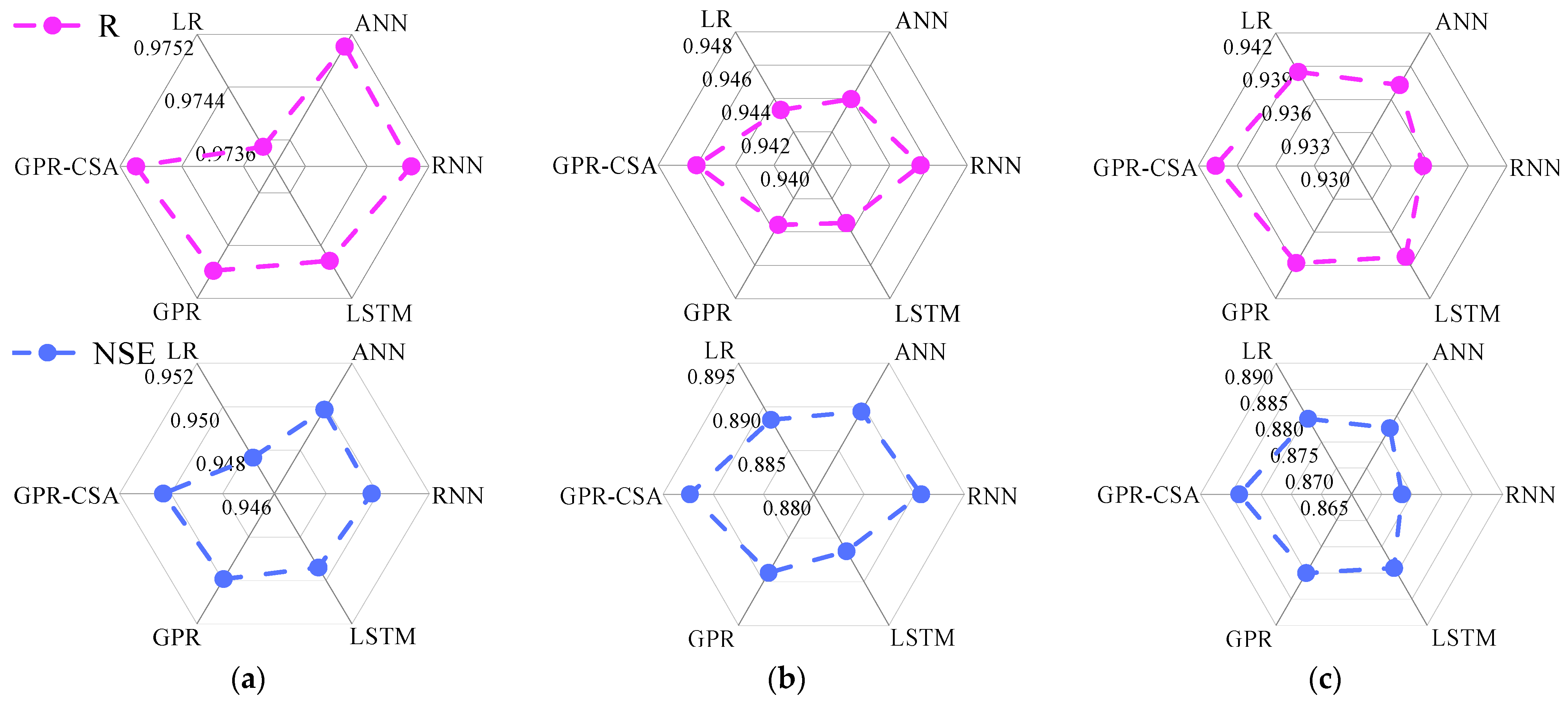
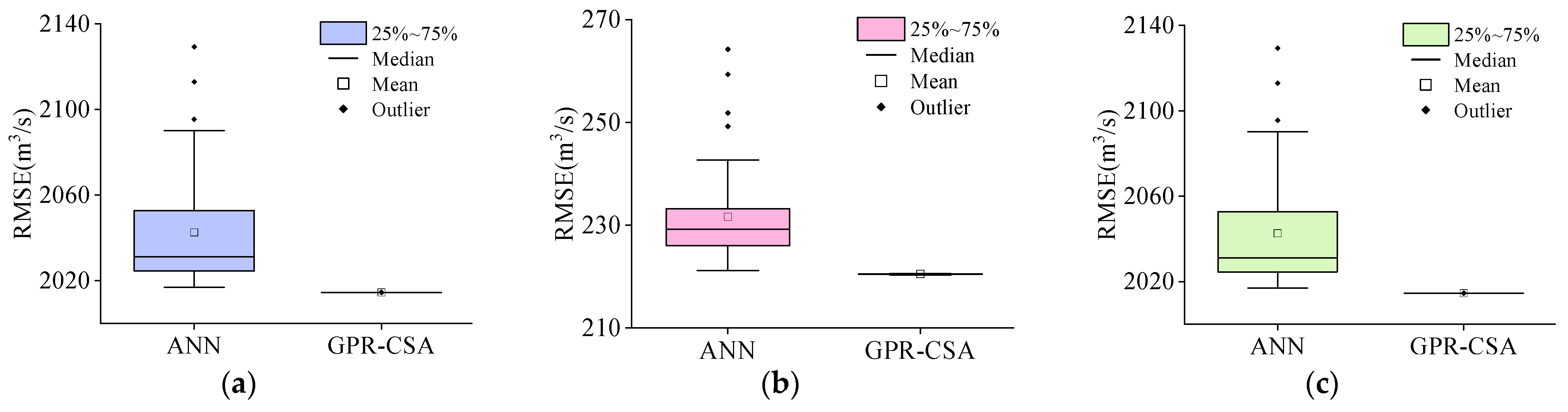
4.4.3. Analysis of the Model Robustness
5. Conclusions
Author Contributions
Funding
Data Availability Statement
Acknowledgments
Conflicts of Interest
References
- Ma, C.; Lian, J.; Wang, J. Short-term optimal operation of Three-gorge and Gezhouba cascade hydropower stations in non-flood season with operation rules from data mining. Energy Convers. Manag. 2013, 65, 616–627. [Google Scholar] [CrossRef]
- Madani, K.; Lund, J.R. California’s Sacramento–San Joaquin Delta Conflict: From Cooperation to Chicken. J. Water Resour. Plan. Manag. 2012, 138, 90–99. [Google Scholar] [CrossRef]
- Zheng, F.; Qi, Z.; Bi, W.; Zhang, T.; Yu, T.; Shao, Y. Improved Understanding on the Searching Behavior of NSGA-II Operators Using Run-Time Measure Metrics with Application to Water Distribution System Design Problems. Water Resour. Manag. 2017, 31, 1121–1138. [Google Scholar] [CrossRef]
- Chen, X.; Huang, J.; Han, Z.; Gao, H.; Liu, M.; Li, Z.; Liu, X.; Li, Q.; Qi, H.; Huang, Y. The importance of short lag-time in the runoff forecasting model based on long short-term memory. J. Hydrol. 2020, 589, 125359. [Google Scholar] [CrossRef]
- Zhang, J.; Chen, X.; Khan, A.; Zhang, Y.-K.; Kuang, X.; Liang, X.; Taccari, M.L.; Nuttall, J. Daily runoff forecasting by deep recursive neural network. J. Hydrol. 2021, 596, 126067. [Google Scholar] [CrossRef]
- He, Y.; Fan, H.; Lei, X.; Wan, J. A runoff probability density prediction method based on B-spline quantile regression and kernel density estimation. Appl. Math. Model. 2021, 93, 852–867. [Google Scholar] [CrossRef]
- Bai, T.; Chang, J.-X.; Chang, F.-J.; Huang, Q.; Wang, Y.-M.; Chen, G.-S. Synergistic gains from the multi-objective optimal operation of cascade reservoirs in the Upper Yellow River basin. J. Hydrol. 2015, 523, 758–767. [Google Scholar] [CrossRef]
- Chang, J.; Wang, X.; Li, Y.; Wang, Y.; Zhang, H. Hydropower plant operation rules optimization response to climate change. Energy 2018, 160, 886–897. [Google Scholar] [CrossRef]
- Liu, D.; Guo, S.; Wang, Z.; Liu, P.; Yu, X.; Zhao, Q.; Zou, H. Statistics for sample splitting for the calibration and validation of hydrological models. Stoch. Environ. Res. Risk Assess. 2018, 32, 3099–3116. [Google Scholar] [CrossRef]
- Liu, P.; Li, L.; Guo, S.; Xiong, L.; Zhang, W.; Zhang, J.; Xu, C.-Y. Optimal design of seasonal flood limited water levels and its application for the Three Gorges Reservoir. J. Hydrol. 2015, 527, 1045–1053. [Google Scholar] [CrossRef]
- Jiang, Z.; Wu, W.; Qin, H.; Hu, D.; Zhang, H. Optimization of fuzzy membership function of runoff forecasting error based on the optimal closeness. J. Hydrol. 2019, 570, 51–61. [Google Scholar] [CrossRef]
- Xie, T.; Zhang, G.; Hou, J.; Xie, J.; Lv, M.; Liu, F. Hybrid forecasting model for non-stationary daily runoff series: A case study in the Han River Basin, China. J. Hydrol. 2019, 577, 123915. [Google Scholar] [CrossRef]
- Zhang, Q.; Wang, B.-D.; He, B.; Peng, Y.; Ren, M.-L. Singular Spectrum Analysis and ARIMA Hybrid Model for Annual Runoff Forecasting. Water Resour. Manag. 2011, 25, 2683–2703. [Google Scholar] [CrossRef]
- Taherei Ghazvinei, P.; Hassanpour Darvishi, H.; Mosavi, A.; Yusof, K.B.W.; Alizamir, M.; Shamshirband, S.; Chau, K.W. Sugarcane growth prediction based on meteorological parameters using extreme learning machine and artificial neural network. Eng. Appl. Comp. Fluid. 2018, 12, 738–749. [Google Scholar] [CrossRef]
- Taormina, R.; Chau, K.-W.; Sivakumar, B. Neural network river forecasting through baseflow separation and binary-coded swarm optimization. J. Hydrol. 2015, 529, 1788–1797. [Google Scholar] [CrossRef]
- Wang, W.-C.; Chau, K.-W.; Xu, D.-M.; Chen, X.-Y. Improving Forecasting Accuracy of Annual Runoff Time Series Using ARIMA Based on EEMD Decomposition. Water Resour. Manag. 2015, 29, 2655–2675. [Google Scholar] [CrossRef]
- Yang, T.; Liu, X.; Wang, L.; Bai, P.; Li, J. Simulating Hydropower Discharge using Multiple Decision Tree Methods and a Dynamical Model Merging Technique. J. Water Resour. Plan. Manag. 2020, 146, 04019072. [Google Scholar] [CrossRef]
- Zhao, T.; Bennett, J.-C.; Wang, Q.-J.; Schepen, A.; Wood, A.W.; Robertson, D.E.; Ramos, M.H. How suitable is quantile mapping for postprocessing GCM precipitation forecasts? J. Clim. 2017, 30, 3185–3196. [Google Scholar] [CrossRef]
- Gao, S.; Huang, Y.; Zhang, S.; Han, J.; Wang, G.; Zhang, M.; Lin, Q. Short-term runoff prediction with GRU and LSTM networks without requiring time step optimization during sample generation. J. Hydrol. 2020, 589, 125188. [Google Scholar] [CrossRef]
- Huo, W.; Li, Z.; Zhang, K.; Wang, J.; Yao, C. GA-PIC: An improved Green-Ampt rainfall-runoff model with a physically based infiltration distribution curve for semi-arid basins. J. Hydrol. 2020, 586, 124900. [Google Scholar] [CrossRef]
- Asante-Okyere, S.; Shen, C.; Ziggah, Y.Y.; Rulegeya, M.M.; Zhu, X. Investigating the Predictive Performance of Gaussian Process Regression in Evaluating Reservoir Porosity and Permeability. Energies 2018, 11, 3261. [Google Scholar] [CrossRef]
- Maritz, J.; Lubbe, F.; Lagrange, L. A Practical Guide to Gaussian Process Regression for Energy Measurement and Verification within the Bayesian Framework. Energies 2018, 11, 935. [Google Scholar] [CrossRef]
- Alizadeh, Z.; Yazdi, J.; Kim, J.H.; Al-Shamiri, A.K. Assessment of Machine Learning Techniques for Monthly Flow Prediction. Water 2018, 10, 1676. [Google Scholar] [CrossRef]
- Taki, M.; Rohani, A.; Soheili-Fard, F.; Abdeshahi, A. Assessment of energy consumption and modeling of output energy for wheat production by neural network (MLP and RBF) and Gaussian process regression (GPR) models. J. Clean. Prod. 2018, 172, 3028–3041. [Google Scholar] [CrossRef]
- Campos-Taberner, M.; García-Haro, F.J.; Camps-Valls, G.; Grau-Muedra, G.; Nutini, F.; Busetto, L.; Katsantonis, D.; Stavrakoudis, D.; Minakou, C.; Gatti, L.; et al. Exploitation of SAR and Optical Sentinel Data to Detect Rice Crop and Estimate Seasonal Dynamics of Leaf Area Index. Remote Sens. 2017, 9, 248. [Google Scholar] [CrossRef]
- Chang, W.; Chen, X. Monthly rainfall-runoff modeling at watershed scale: A comparative study of data-driven and theory-driven approaches. Water 2018, 10, 1116. [Google Scholar] [CrossRef]
- Fang, D.; Zhang, X.; Yu, Q.; Jin, T.C.; Tian, L. A novel method for carbon dioxide emission forecasting based on improved Gaussian processes regression. J. Clean. Prod. 2018, 173, 143–150. [Google Scholar] [CrossRef]
- Sun, A.Y.; Wang, D.; Xu, X. Monthly streamflow forecasting using Gaussian Process Regression. J. Hydrol. 2014, 511, 72–81. [Google Scholar] [CrossRef]
- Yan, J.; Li, K.; Bai, E.; Yang, Z.; Foley, A. Time series wind power forecasting based on variant Gaussian Process and TLBO. Neurocomputing 2016, 189, 135–144. [Google Scholar] [CrossRef]
- Feng, Z.-K.; Niu, W.-J.; Shi, P.-F.; Yang, T. Adaptive Neural-Based Fuzzy Inference System and Cooperation Search Algorithm for Simulating and Predicting Discharge Time Series Under Hydropower Reservoir Operation. Water Resour. Manag. 2022, 36, 2795–2812. [Google Scholar] [CrossRef]
- Liu, X.; Paritosh, P.; Awalgaonkar, N.M.; Bilionis, I.; Karava, P. Model predictive control under forecast uncertainty for optimal operation of buildings with integrated solar systems. Sol. Energy 2018, 171, 953–970. [Google Scholar] [CrossRef]
- Hermans, T.; Oware, E.; Caers, J. Direct prediction of spatially and temporally varying physical properties from time-lapse electrical resistance data. Water Resour. Res. 2016, 52, 7262–7283. [Google Scholar] [CrossRef]
- Liu, H.; Cai, J.; Ong, Y.-S. Remarks on multi-output Gaussian process regression. Knowl.-Based Syst. 2018, 144, 102–121. [Google Scholar] [CrossRef]
- Feng, Z.-K.; Huang, Q.-Q.; Niu, W.-J.; Yang, T.; Wang, J.-Y.; Wen, S.-P. Multi-step-ahead solar output time series prediction with gate recurrent unit neural network using data decomposition and cooperation search algorithm. Energy 2022, 261, 125217. [Google Scholar] [CrossRef]
- Feng, Z.-K.; Niu, W.-J.; Wan, X.-Y.; Xu, B.; Zhu, F.-L.; Chen, J. Hydrological time series forecasting via signal decomposition and twin support vector machine using cooperation search algorithm for parameter identification. J. Hydrol. 2022, 612, 128213. [Google Scholar] [CrossRef]
- Feng, Z.-K.; Shi, P.-F.; Yang, T.; Niu, W.-J.; Zhou, J.-Z.; Cheng, C.-T. Parallel cooperation search algorithm and artificial intelligence method for streamflow time series forecasting. J. Hydrol. 2022, 606, 127434. [Google Scholar] [CrossRef]


| Station | Method | Training | Testing | ||||||
|---|---|---|---|---|---|---|---|---|---|
| RMSE | MAE | R | NSE | RMSE | MAE | R | NSE | ||
| SX | LR | 2179.8125 | 1087.0266 | 0.9779 | 0.9564 | 2067.5276 | 967.7999 | 0.9735 | 0.9477 |
| ANN | 2141.9027 | 1081.5492 | 0.9789 | 0.9579 | 2023.4121 | 953.2562 | 0.9750 | 0.9499 | |
| RNN | 2132.8611 | 1092.9085 | 0.9790 | 0.9582 | 2025.3833 | 959.7314 | 0.9750 | 0.9498 | |
| LSTM | 2116.3733 | 1059.8781 | 0.9792 | 0.9589 | 2032.6758 | 931.1892 | 0.9746 | 0.9494 | |
| GPR | 2133.3407 | 1074.1451 | 0.9789 | 0.9582 | 2021.9179 | 933.6396 | 0.9748 | 0.9499 | |
| GPR-CSA | 2090.5676 | 1040.6587 | 0.9797 | 0.9599 | 2014.4942 | 910.2308 | 0.9750 | 0.9503 | |
| LYX | LR | 146.5653 | 84.6916 | 0.9491 | 0.9008 | 224.2732 | 132.8247 | 0.9433 | 0.8885 |
| ANN | 145.0672 | 85.5849 | 0.9503 | 0.9028 | 223.3189 | 131.6143 | 0.9440 | 0.8895 | |
| RNN | 143.9679 | 81.9808 | 0.9509 | 0.9042 | 222.0857 | 128.5580 | 0.9456 | 0.8907 | |
| LSTM | 145.0215 | 83.2984 | 0.9502 | 0.9028 | 226.2795 | 130.8222 | 0.9435 | 0.8865 | |
| GPR | 146.1233 | 84.2844 | 0.9494 | 0.9013 | 223.8168 | 132.3147 | 0.9436 | 0.8890 | |
| GPR-CSA | 143.7597 | 81.5556 | 0.9511 | 0.9045 | 220.4119 | 127.9265 | 0.9460 | 0.8923 | |
| TNH | LR | 156.1520 | 90.5924 | 0.9491 | 0.9008 | 225.4124 | 128.9411 | 0.9385 | 0.8794 |
| ANN | 157.7914 | 93.3550 | 0.9482 | 0.8987 | 227.0591 | 134.6547 | 0.9373 | 0.8776 | |
| RNN | 159.8438 | 92.2203 | 0.9466 | 0.8961 | 231.0292 | 133.9100 | 0.9355 | 0.8733 | |
| LSTM | 155.8957 | 90.6369 | 0.9493 | 0.9011 | 225.7327 | 130.1097 | 0.9382 | 0.8791 | |
| GPR | 155.6946 | 90.1865 | 0.9494 | 0.9014 | 224.8368 | 128.4849 | 0.9388 | 0.8800 | |
| GPR-CSA | 153.7759 | 88.1168 | 0.9507 | 0.9038 | 221.4671 | 125.6045 | 0.9407 | 0.8836 |
| Station | Method | Training | Testing | ||||||
|---|---|---|---|---|---|---|---|---|---|
| RMSE | MAE | R | NSE | RMSE | MAE | R | NSE | ||
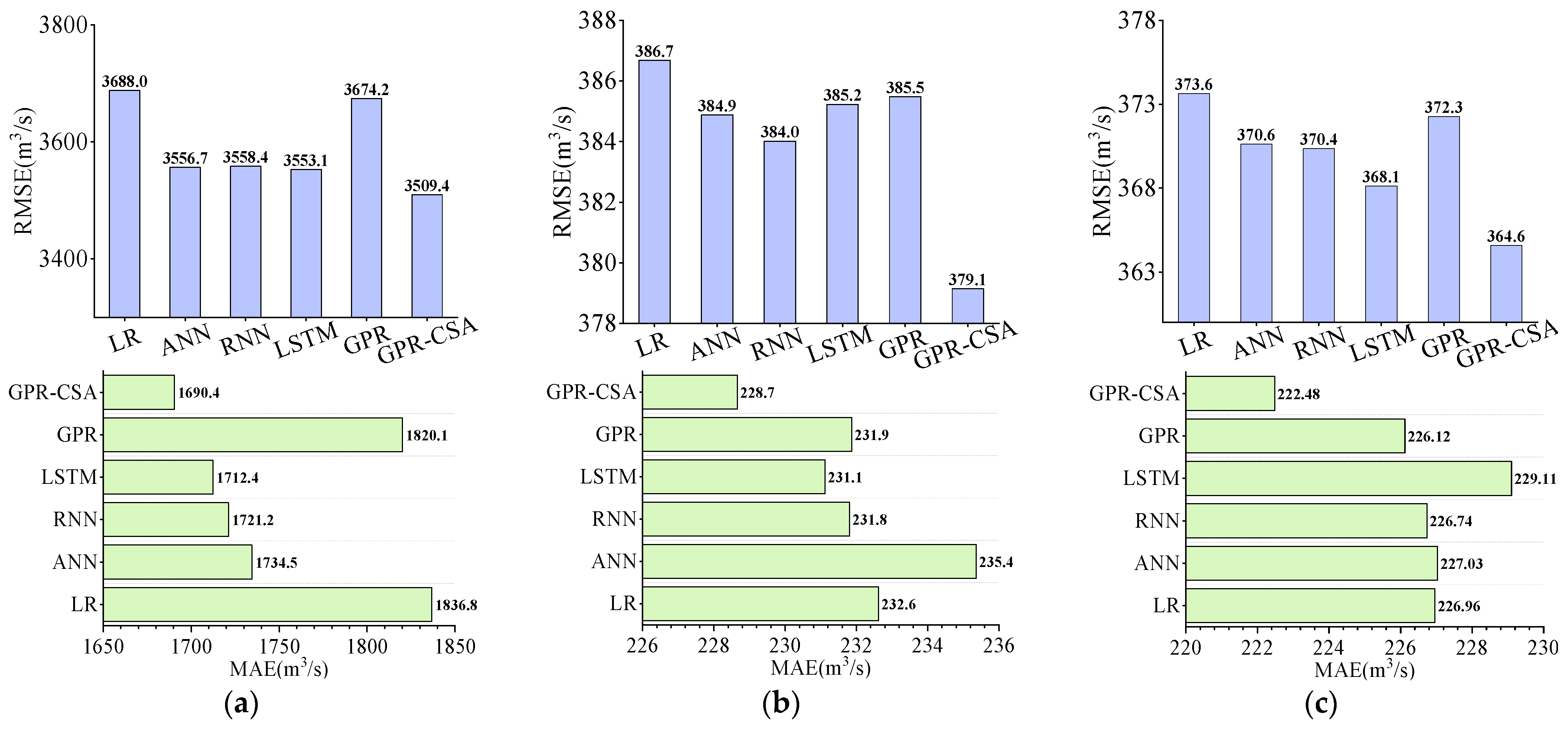
| SX | LR | 3942.6985 | 2057.7949 | 0.9260 | 0.8574 | 3687.9804 | 1836.8307 | 0.9131 | 0.8334 |
| ANN | 3796.7594 | 1985.0689 | 0.9316 | 0.8678 | 3556.6630 | 1734.4789 | 0.9204 | 0.8451 | |
| RNN | 3785.2346 | 1965.4362 | 0.9320 | 0.8686 | 3558.4027 | 1721.2091 | 0.9203 | 0.8449 | |
| LSTM | 3772.2812 | 1952.1839 | 0.9325 | 0.8695 | 3553.0890 | 1712.4415 | 0.9205 | 0.8454 | |
| GPR | 3921.7630 | 2042.2414 | 0.9268 | 0.8589 | 3674.1653 | 1820.1443 | 0.9138 | 0.8347 | |
| GPR-CSA | 3717.3493 | 1926.0842 | 0.9345 | 0.8733 | 3509.4283 | 1690.3785 | 0.9222 | 0.8492 | |
| LYX | LR | 244.1420 | 151.6329 | 0.8515 | 0.7250 | 386.6832 | 232.6207 | 0.8226 | 0.6686 |
| ANN | 242.7675 | 149.0092 | 0.8534 | 0.7281 | 384.8749 | 235.3607 | 0.8268 | 0.6717 | |
| RNN | 237.6878 | 144.4694 | 0.8599 | 0.7393 | 384.0141 | 231.8109 | 0.8279 | 0.6732 | |
| LSTM | 237.6402 | 143.2128 | 0.8599 | 0.7394 | 385.2297 | 231.1241 | 0.8308 | 0.6711 | |
| GPR | 242.9637 | 150.3755 | 0.8530 | 0.7276 | 385.4811 | 231.8700 | 0.8238 | 0.6707 | |
| GPR-CSA | 236.6189 | 142.8215 | 0.8612 | 0.7417 | 379.1407 | 228.6581 | 0.8330 | 0.6814 | |
| TNH | LR | 257.0790 | 161.1098 | 0.8553 | 0.7315 | 373.6444 | 226.9604 | 0.8222 | 0.6687 |
| ANN | 254.3070 | 156.0087 | 0.8587 | 0.7373 | 370.6303 | 227.0324 | 0.8258 | 0.6740 | |
| RNN | 254.4948 | 158.7407 | 0.8584 | 0.7369 | 370.3550 | 226.7389 | 0.8251 | 0.6745 | |
| LSTM | 254.8199 | 156.2293 | 0.8581 | 0.7362 | 368.1236 | 229.1052 | 0.8289 | 0.6784 | |
| GPR | 255.8652 | 160.0530 | 0.8568 | 0.7340 | 372.2691 | 226.1210 | 0.8235 | 0.6711 | |
| GPR-CSA | 250.4350 | 154.1625 | 0.8633 | 0.7452 | 364.5931 | 222.4808 | 0.8313 | 0.6845 |
| Station | Method | Training | Testing | ||||||
|---|---|---|---|---|---|---|---|---|---|
| RMSE | MAE | R | NSE | RMSE | MAE | R | NSE | ||
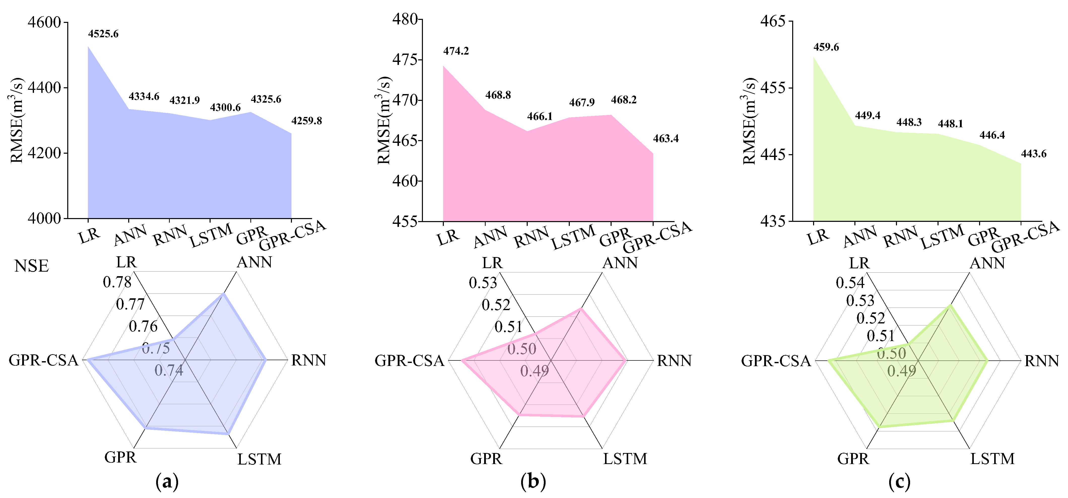
| SX | LR | 4793.3394 | 2588.2535 | 0.8885 | 0.7895 | 4525.6364 | 2391.3104 | 0.8660 | 0.7492 |
| ANN | 4563.0691 | 2454.2423 | 0.8997 | 0.8092 | 4334.6286 | 2254.3684 | 0.8798 | 0.7699 | |
| RNN | 4542.2538 | 2438.6045 | 0.9005 | 0.8109 | 4321.9372 | 2237.3552 | 0.8807 | 0.7713 | |
| LSTM | 4532.9915 | 2452.7204 | 0.9010 | 0.8117 | 4300.6186 | 2247.8933 | 0.8817 | 0.7735 | |
| GPR | 4548.5324 | 2464.9372 | 0.9002 | 0.8104 | 4325.5558 | 2261.5996 | 0.8799 | 0.7709 | |
| GPR-CSA | 4492.1895 | 2424.8873 | 0.9028 | 0.8151 | 4259.7887 | 2204.6138 | 0.8838 | 0.7778 | |
| LYX | LR | 306.6492 | 203.0209 | 0.7524 | 0.5662 | 474.2153 | 306.9632 | 0.7212 | 0.5021 |
| ANN | 292.4584 | 187.3703 | 0.7781 | 0.6054 | 468.7709 | 295.1098 | 0.7445 | 0.5135 | |
| RNN | 290.3365 | 184.7736 | 0.7818 | 0.6111 | 466.1477 | 292.4331 | 0.7454 | 0.5189 | |
| LSTM | 292.5871 | 186.6877 | 0.7779 | 0.6050 | 467.8508 | 294.4701 | 0.7477 | 0.5154 | |
| GPR | 295.2664 | 189.9242 | 0.7732 | 0.5978 | 468.1844 | 297.8071 | 0.7380 | 0.5147 | |
| GPR-CSA | 279.4007 | 172.0490 | 0.7999 | 0.6398 | 463.4016 | 289.1666 | 0.7514 | 0.5245 | |
| TNH | LR | 325.8074 | 214.8081 | 0.7541 | 0.5686 | 459.6293 | 298.6075 | 0.7175 | 0.4992 |
| ANN | 315.2876 | 201.6766 | 0.7721 | 0.5960 | 449.3503 | 292.8334 | 0.7376 | 0.5214 | |
| RNN | 315.5895 | 204.7256 | 0.7716 | 0.5953 | 448.3488 | 293.8328 | 0.7339 | 0.5235 | |
| LSTM | 316.0069 | 204.4948 | 0.7709 | 0.5942 | 448.1143 | 294.4648 | 0.7371 | 0.5240 | |
| GPR | 314.9528 | 203.3613 | 0.7726 | 0.5969 | 446.4302 | 291.9147 | 0.7374 | 0.5276 | |
| GPR-CSA | 310.9775 | 200.1707 | 0.7794 | 0.6070 | 443.6498 | 288.7442 | 0.7468 | 0.5334 |
| Station | Kernel | Method | Training | Testing | ||||||
|---|---|---|---|---|---|---|---|---|---|---|
| RMSE | MAE | R | NSE | RMSE | MAE | R | NSE | |||
| SX | kernel1 | GPR | 2176.7778 | 1082.6186 | 0.9780 | 0.9565 | 2064.6345 | 966.2568 | 0.9736 | 0.9478 |
| GPR-CSA | 2090.7676 | 1040.6310 | 0.9797 | 0.9599 | 2015.0046 | 910.6999 | 0.9750 | 0.9503 | ||
| Improvement | 3.95% | 3.88% | 0.18% | 0.35% | 2.40% | 5.75% | 0.15% | 0.26% | ||
| kernel2 | GPR | 2133.3397 | 1073.5378 | 0.9789 | 0.9582 | 2021.9094 | 933.6112 | 0.9748 | 0.9499 | |
| GPR-CSA | 2090.8223 | 1040.6587 | 0.9797 | 0.9599 | 2015.0183 | 910.7315 | 0.9750 | 0.9503 | ||
| Improvement | 1.99% | 3.06% | 0.09% | 0.17% | 0.34% | 2.45% | 0.02% | 0.04% | ||
| kernel3 | GPR | 2133.3407 | 1074.1451 | 0.9789 | 0.9582 | 2021.9179 | 933.6396 | 0.9748 | 0.9499 | |
| GPR-CSA | 2090.5676 | 1040.6587 | 0.9797 | 0.9599 | 2014.4942 | 910.2308 | 0.9750 | 0.9503 | ||
| Improvement | 2.00% | 3.12% | 0.09% | 0.17% | 0.37% | 2.51% | 0.02% | 0.04% | ||
| LYX | kernel1 | GPR | 146.4337 | 84.6313 | 0.9492 | 0.9009 | 224.3537 | 132.7793 | 0.9433 | 0.8884 |
| GPR-CSA | 143.7545 | 81.5415 | 0.9511 | 0.9045 | 220.3405 | 127.8677 | 0.9460 | 0.8924 | ||
| Improvement | 1.83% | 3.65% | 0.20% | 0.40% | 1.79% | 3.70% | 0.29% | 0.45% | ||
| kernel2 | GPR | 146.2409 | 84.4382 | 0.9493 | 0.9012 | 224.1000 | 132.5332 | 0.9434 | 0.8887 | |
| GPR-CSA | 143.7740 | 81.5776 | 0.9511 | 0.9045 | 220.4450 | 127.9491 | 0.9460 | 0.8923 | ||
| Improvement | 1.69% | 3.39% | 0.18% | 0.37% | 1.63% | 3.46% | 0.27% | 0.41% | ||
| kernel3 | GPR | 146.1233 | 84.2844 | 0.9494 | 0.9013 | 223.8168 | 132.3147 | 0.9436 | 0.8890 | |
| GPR-CSA | 143.7597 | 81.5556 | 0.9511 | 0.9045 | 220.4119 | 127.9265 | 0.9460 | 0.8923 | ||
| Improvement | 1.62% | 3.24% | 0.18% | 0.35% | 1.52% | 3.32% | 0.26% | 0.38% | ||
| TNH | kernel1 | GPR | 156.0139 | 90.5336 | 0.9492 | 0.9010 | 225.3258 | 128.9740 | 0.9385 | 0.8795 |
| GPR-CSA | 153.7880 | 88.1002 | 0.9507 | 0.9038 | 221.3923 | 125.5130 | 0.9407 | 0.8837 | ||
| Improvement | 1.43% | 2.69% | 0.16% | 0.31% | 1.75% | 2.68% | 0.23% | 0.47% | ||
| kernel2 | GPR | 155.8151 | 90.3433 | 0.9493 | 0.9012 | 225.0535 | 128.7429 | 0.9387 | 0.8798 | |
| GPR-CSA | 153.7588 | 88.0945 | 0.9507 | 0.9038 | 221.3747 | 125.5502 | 0.9407 | 0.8837 | ||
| Improvement | 1.32% | 2.49% | 0.14% | 0.29% | 1.63% | 2.48% | 0.22% | 0.44% | ||
| kernel3 | GPR | 155.6946 | 90.1865 | 0.9494 | 0.9014 | 224.8368 | 128.4849 | 0.9388 | 0.8800 | |
| GPR-CSA | 153.7759 | 88.1168 | 0.9507 | 0.9038 | 221.4671 | 125.6045 | 0.9407 | 0.8836 | ||
| Improvement | 1.23% | 2.29% | 0.13% | 0.27% | 1.50% | 2.24% | 0.20% | 0.41% |
Disclaimer/Publisher’s Note: The statements, opinions and data contained in all publications are solely those of the individual author(s) and contributor(s) and not of MDPI and/or the editor(s). MDPI and/or the editor(s) disclaim responsibility for any injury to people or property resulting from any ideas, methods, instructions or products referred to in the content. |
© 2023 by the authors. Licensee MDPI, Basel, Switzerland. This article is an open access article distributed under the terms and conditions of the Creative Commons Attribution (CC BY) license (https://creativecommons.org/licenses/by/4.0/).
Share and Cite
Wang, S.; Gong, J.; Gao, H.; Liu, W.; Feng, Z. Gaussian Process Regression and Cooperation Search Algorithm for Forecasting Nonstationary Runoff Time Series. Water 2023, 15, 2111. https://doi.org/10.3390/w15112111
Wang S, Gong J, Gao H, Liu W, Feng Z. Gaussian Process Regression and Cooperation Search Algorithm for Forecasting Nonstationary Runoff Time Series. Water. 2023; 15(11):2111. https://doi.org/10.3390/w15112111
Chicago/Turabian StyleWang, Sen, Jintai Gong, Haoyu Gao, Wenjie Liu, and Zhongkai Feng. 2023. "Gaussian Process Regression and Cooperation Search Algorithm for Forecasting Nonstationary Runoff Time Series" Water 15, no. 11: 2111. https://doi.org/10.3390/w15112111
APA StyleWang, S., Gong, J., Gao, H., Liu, W., & Feng, Z. (2023). Gaussian Process Regression and Cooperation Search Algorithm for Forecasting Nonstationary Runoff Time Series. Water, 15(11), 2111. https://doi.org/10.3390/w15112111