Simulation and Dynamic Properties Analysis of the Anaerobic–Anoxic–Oxic Process in a Wastewater Treatment PLANT Based on Koopman Operator and Deep Learning

Abstract

The accurate simulation of the dynamics of the anaerobic–anoxic–oxic (A2O) process in the biochemical reactions in wastewater treatment plants (WWTPs) is important for system prediction and optimization. Previous studies have used real-time monitoring data of WWTPs to develop data-driven predictive models, but these models cannot be used to provide mathematical analysis of A2O dynamic properties. In this study, we developed a new simulation and analysis method for determining A2O dynamics in biochemical reactions using deep learning and the Koopman operator to address the above problems. This method was validated through data from a real-world WWTP in east China and compared it with the traditional deep learning model. According to the results, the new method achieved high-accuracy prediction. Meanwhile, with the help of the Koopman operator, the new method was able to analyze the asymptotical stability and convergence behavior of the A2O process, which provides a brand-new perspective for the in-depth study of biochemical reactor dynamics.

1. Introduction

The anaerobic–anoxic–oxic (A2O) process in biochemical reactors of wastewater treatment (WWT) is important in urban water systems [1]. Mechanism models of A2O have been developed for dynamic prediction and control [2,3,4,5]. However, they are built on fixed parameters, equations, and model assumptions, which lack the flexibility and adaptability to respond to external environmental changes and stochastic perturbation in real-world conditions. With the widespread adoption of intelligent devices, data monitoring systems, and SCADA, a large amount of dynamic data for the A2O process has gradually accumulated. As a result, the construction of A2O dynamic models based on data-driven methods has gradually emerged, e.g., linear models [6], machine learning [7], artificial neural networks [8,9], and deep learning models [10]. These methods establish simulation and prediction models based on measured data that records various random events and perturbation factors. Therefore, they are more generalizable and adaptable to real-world situations.

However, existing data-driven models, especially deep learning models, are black-box models that lack interpretability and cannot be used to analyze the dynamic properties of the A2O process in a biochemical reactor. This is consistent with existing research on the dynamic properties based on deep learning and some data-driven methods [11,12,13,14]. Therefore, finding the intersection point between data-driven methods and dynamic analysis through appropriate modeling for A2O dynamics is necessary.

The Koopman operator provides a solution to the above problem. For a given nonlinear dynamic system, obtaining its Koopman operator can help us find its eigenvalues, thereby revealing its linear structure and analyzing its dynamic properties mathematically [15,16,17,18,19,20,21]. The theory and correlated methods have been widely used in model prediction [22], data fusion [23], fluid dynamics [24,25], and system control [26,27,28]. The methods used to find the Koopman operator of a given system include purely mathematical methods [29] and data-driven methods [30,31]. In recent years, deep learning has also been used to find the Koopman operator of a given nonlinear dynamic system, providing a new direction for mathematical analysis and system simulation [32,33,34].

This study constructed a new data-driven simulation model of A2O process in WWTP to solve the above problem. This model provides accuracy prediction and mathematical analysis for A2O dynamics using Koopman operator and deep learning. Based on this, a deep learning model that takes into account both dynamic properties analysis and accurate predictions is built for A2O to provide new insight into the dynamics of A2O from a mathematical perspective.

2. Materials and Methods

Deep learning and the Koopman operator were applied to establish a new simulation method and a dynamic analysis method for the A2O process in this study. First, the data for an A2O process in a WWTP in eastern China were collected and cleaned. Based on the cleaned dataset, a traditional deep-learning method was used to construct a simulation model as a baseline model for A2O dynamic prediction. Then, a new simulation model based on the combination of deep learning and the Koopman operator was designed and used to provide a mathematical analysis method for A2O dynamic properties. The following sections provide details on the methods.

2.1. Case Study and Data

The case study is a real-world WWTP located in eastern China. The WWTP adopts the A2O process, with a design flow rate of 800,000 m³/d and 8 groups of bioreactors, each with a capacity of 100,000 m³/d and can operate independently. The A2O process uses microorganisms to remove organic pollutants, ammonia, and phosphorus in water through anaerobic, anoxic, and aerobic treatment processes, so as to meet the discharge standards [35]. The aerobic section of the biochemical reactor uses blowers at the bottom of the reactor to provide oxygen for microorganisms to grow, consume organic pollutants, and prevent activated sludge from settling. This study only focuses on bioreactor no. 1, which has an online data monitoring system. It has three parts, anaerobic, anoxic, and oxic; their volumes are 55,696 m³, 133,670 m³, and 321,680 m³, respectively.

This study collected the data for the bioreactor no.1 in the WWTP from 1 May 2020, at 00:00 to 21 October 2020, at 14:40. The monitoring sample frequency was 5 min. Four types of data (state, control, inflow, and outflow) were collected. Their information is given in

Table 1. Statistic information of A2O process data.

Data Name and Unit	Type	Maximum	Minimum	Average	Median
Aerobic MLSS (g/L)	State	5.733	2.515	3.878	3.975
Anaerobic MLSS (g/L)		6.111	0.774	3.455	3.505
Anoxic MLSS (g/L)		6.405	2.861	3.966	3.873
Anaerobic ORP		−226.223	−480.649	−421.539	−447.093
Anoxic ORP		−20.668	−244.451	−98.212	−93.690
Aerobic ${NO}_3^{-}$ (mg/L)		32.873	1.546	9.287	3.348
Aerobic DO (mg/L)		7.150	0.803	3.109	3.015
Aeration volume (m3/min)	Control	29.755	18.277	23.892	23.961
Qr (m3/s)		2.332	0.906	1.915	1.962
Qsr (m3/s)		5.534	4.399	4.834	4.815
COD (mg/L)	Influent/ Inflow	650.329	49.315	270.051	229.321
TN (mg/L)		44.354	3.579	26.233	26.345
TP (mg/L)		7.950	0.185	3.514	3.448
T (°C)		30.922	21.351	26.054	26.386
SS (mg/L)		67.341	0.000	7.506	3.789
Flow (m3/s)		3.203	1.144	2.587	2.628
COD (mg/L)	Effluent/ Outflow	53.355	18.252	27.431	22.983
TN (mg/L)		13.011	4.428	6.909	6.594
TP (mg/L)		0.437	0.285	0.354	0.353
${NH}_4^{+}-N$ (mg/L)		0.179	0.054	0.100	0.091
${NO}_3^{-}$ (mg/L)		12.286	3.898	6.232	5.904

. The state data represent the water quality data inside the bioreactor, which included dissolved oxygen (DO) in the aerobic section, oxidation–reduction potential (ORP) of the anaerobic and anoxic sections, nitrate nitrogen (${NO}_3^{-}$) of the aerobic section, and mixed liquor suspended solids concentration (MLSS) of the anaerobic, anoxic, and aerobic sections. The control data represent the data related to aeration (aeration volume), internal recirculation flow rate (Qr), and sludge internal recycle flow rate (Qsr). The inflow data represent the data of inflow water, which includes chemical oxygen demand (COD), total nitrogen (TN), total phosphorus (TP), water temperature (T), suspended substance (SS), and flow rate (flow). The outflow data represent the data of outflow water, which includes chemical oxygen demand (COD), total nitrogen (TN), total phosphorus (TP), ammonia nitrogen (${NH}_4^{+}-N$), nitrate nitrogen (${NO}_3^{-}$). The original COD, TP, and TN data were measured every two hours and their time series data comprised the same values every two hours, resulting in the original data being shown in a stepwise manner.

Due to the presence of outliers in the original data, data cleaning was performed. Based on the PauTa Criterion, extreme outlier data were removed and data were supplemented using interpolation. Firstly, the time interval for data cleaning was determined based on the hydraulic retention time (HRT) of the bio-reactor, and the mean and variance of various state data of the bio-reactor within the time interval were calculated. Then, according to the hypothesis testing PauTa Criterion, extreme outlier data within the time interval was deleted and supplemented using interpolation data. The criterion can be described by Equation (1), and the interpolation is shown in Equation (2), where N represents the time steps in the time interval, ${data}_i$ represents the i-th data point in the time interval, and $\overline{{data}_i}$ represents the supplementing data.

$$\left|V_i\right|>3\sigma ,\sigma =\sqrt{\frac{1}{N}\sum _{i=1}^N{\left({data}_i-\overline{data}\right)}^2}$$

(1)

$$\overline{{data}_i}=\frac{1}{N}\sum _{j=i-\frac{N}{2}}^{i+\frac{N}{2}}{data}_j$$

(2)

After deleting the abnormal data, the moving average method was used to eliminate the small disturbances caused by the anomalies (Equation (3), where $\widehat{{data}_t}$ represented the data that have been corrected, n was the time span of the moving average and was 100 in this study). After being processed, the data relieved the impact of abnormal and disruptive values, providing a foundation for subsequent analysis and modeling. In addition, all the data were smoothed through this process. The specific details and statistical results of the cleansed dataset are shown in the table below.

$$\widehat{{data}_t}=\frac{1}{n}\sum _{j=t-\frac{n}{2}}^{t+\frac{n}{2}}{data}_i$$

(3)

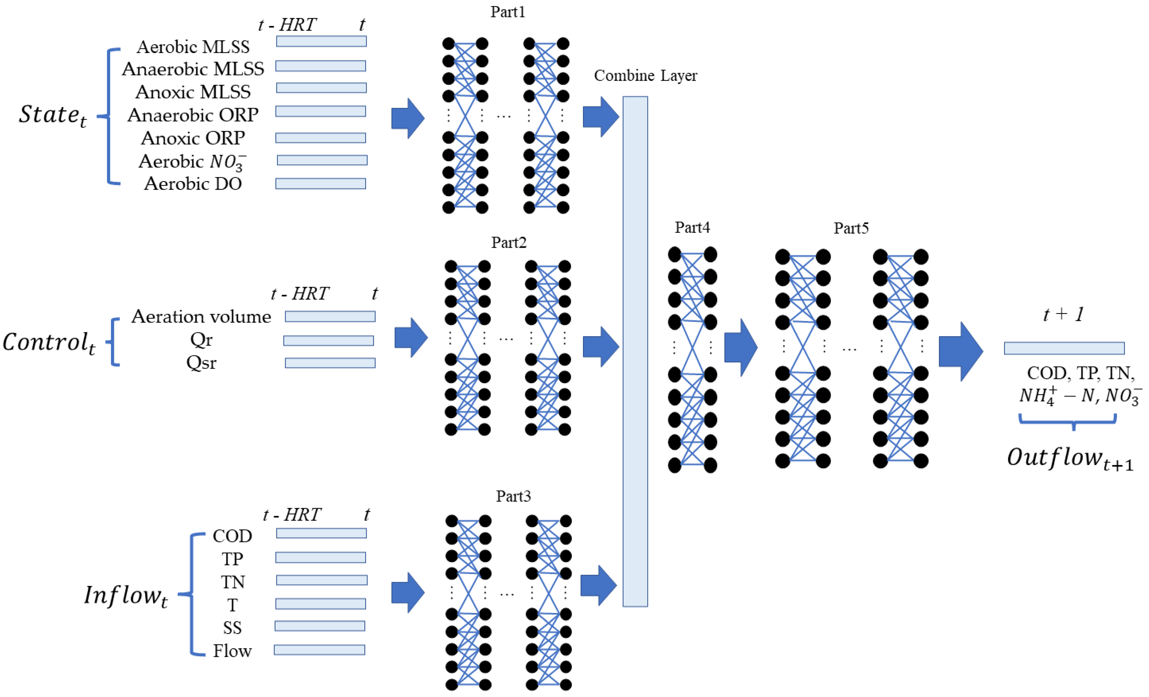
2.2. Deep Learning for A2O Process Simulation and Prediction

The above data contain information on the influent, anaerobic, anoxic, and aerobic reaction processes, and effluent quality, covering the elements of carbon, nitrogen, and phosphorus, all of which have an impact on the dynamic of A2O process. Therefore, this study used the above data to construct a deep learning-based simulation model that focused on the inflow–state–control–outflow of A2O process. The inflow, state data, and control data were used as inputs for the simulation model, and the outflow data were used as the outputs of the simulation model. All input data were time series data for a period of time with a time span of hydraulic retention time (HRT), which was 7 h in this study. The model predicted the outflow data for the next half hour.

Accordingly, the deep learning-based model (called DNN in this study) can be described as Equation (4), where ${State}_t$, ${Control}_t$, ${Inflow}_t$ are the state, control, and inflow in previous HRT, ${Outflow}_{t+1}$ is the outflow in next half hour and is the output of the model. The training process of DNN is to minimize the loss function based on prediction error Equation (5), where $\overline{{Outflow}_{t+1}}$ is the output of model. All the data for inputs and outputs were normalized to avoid the influence of differences in data magnitude, and the results of the simulation were obtained by renormalization. The formula is shown in Equations (6) and (7), where $DATA$, $DATAmin$, and $DATAmax$ are the original data and its minimum and maximum, $data$ is the normalized data, and $\overline{DATA}$ is the renormalized data.

$${Outflow}_{t+1}=DNN\left({State}_t,{Control}_t,{Inflow}_t|\theta \right)$$

(4)

$$\underset{\theta }{\min }\frac{1}{2}{‖\overline{{Outflow}_{t+1}}-DNN\left({State}_t,{Control}_t,{Inflow}_t|\theta \right)‖}^2+\lambda {‖\theta ‖}^2$$

(5)

$$data=2\frac{DATA-DATAmin}{DATAmax-DATAmin}-1$$

(6)

$$\overline{DATA}=DATAmin+\frac{DATAmax-DATAmin}{2}\left(data+1\right)$$

(7)

DNN is trained using the standard Adam training algorithm [36], with 0.001 initial learning rate and 500 iterations. After training, the model performs prediction by inputting the corresponding state, control, and inflow variables. The structure and parameters of DNN are shown in Figure 1 and

Table 2. Architecture and parameters of deep neural network in DNN.

	Architecture	Activation Function
Part1 (State)	$HRT\times 7$-50-50-50	$tanh\left(x\right)=\frac{e^x-e^{-x}}{e^x+e^{-x}}$
Part2 (Control)	$HRT\times 3$-50-50-50
Part3 (Inflow)	$HRT\times 6$-50-50-50
Part4 (Encoding)	50-50-50-50
Part5 (Outflow)	50-50-5

, respectively.

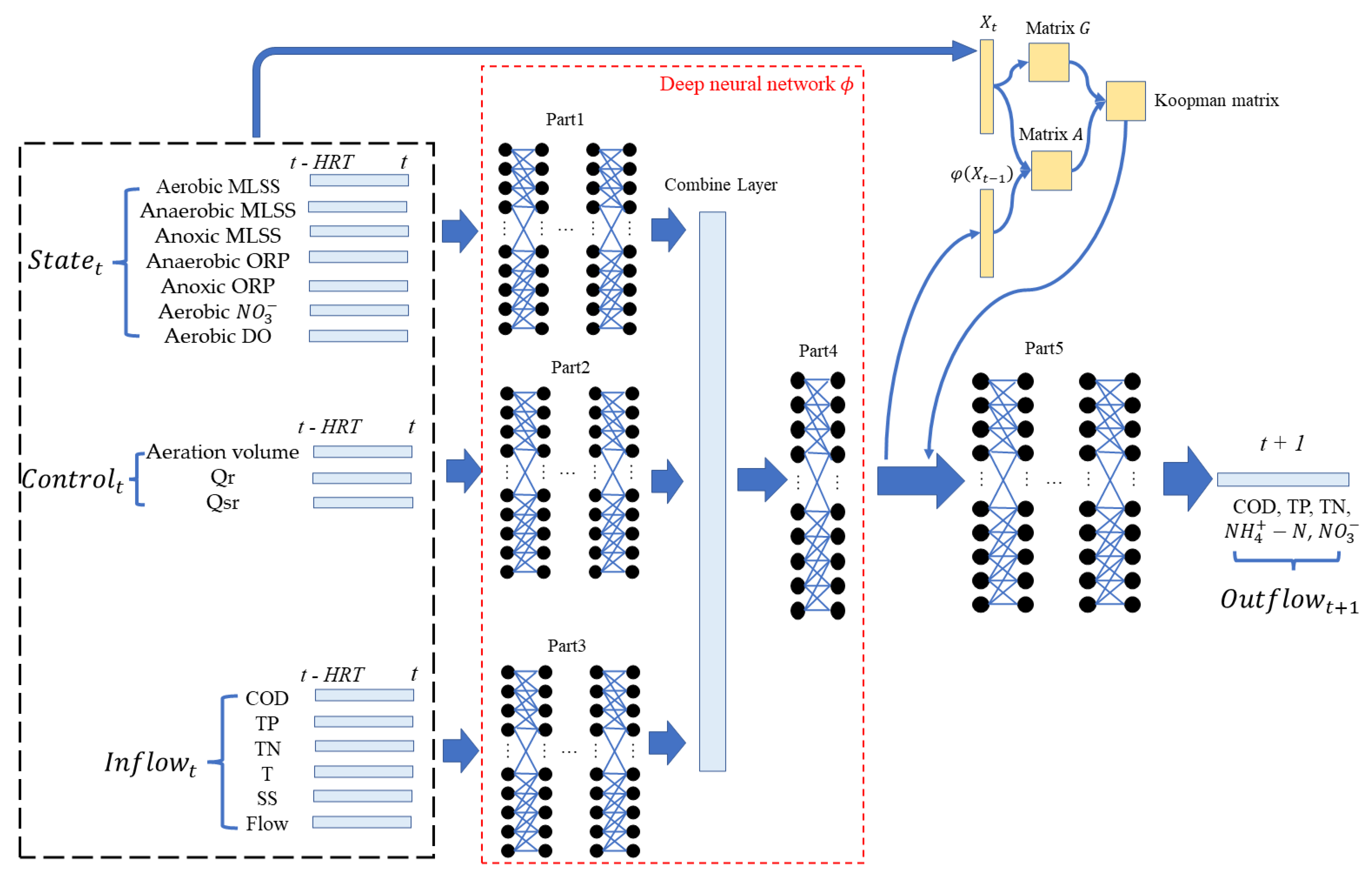
2.3. Koopman Operator and Deep Learning for A2O Process Simulation and Prediction

Due to the lack of interpretability in deep learning methods, it is difficult for DNN to perform in-depth analysis of the A2O process dynamics. In this study, a new A2O dynamic simulation model was constructed by combining Koopman operators and deep learning methods.

2.3.1. Dynamic System and the Koopman Operator

The definition of the Koopman operator and its approximation theory can be found in previous works [32,33]. We only provide a step-by-step introduction in this section. The dynamic of A2O can be described by a nonlinear dynamic system Equation (8), which has a corresponding Koopman operator to describe the evolution of a given observable through a linear system (Equation (9)), where $\kappa$ is Koopman operator and $f$ is observable represented by functions in a Hilbert space [31].

$${Outflow}_{t+1}=F\left({State}_t,{Control}_t,{Inflow}_t\right),$$

(8)

$$\begin{array}{cc}\mathbb{E}\left[{Outflow}_{t+1}\right]\hfill & =\mathbb{E}\left[f\left(F\left({State}_t,{Control}_t,{Inflow}_t\right)\right)\right]\hfill \\ \hfill & =\kappa \mathbb{E}\left[f\left({State}_t,{Control}_t,{Inflow}_t\right)\right]\hfill \end{array}$$

(9)

However, this linear system has an infinite dimension [23,30] and cannot be used for simulation and prediction directly. Thus, its finite dimensional approximation is required. Given a set of dictionary functions $\mathsf{\Psi }=\left[{\psi }_1,{\psi }_2,\dots ,{\psi }_L\right]$, the observable can be written as $f\left(x\left(n\right)\right)=\Xi \mathsf{\Psi }\left(x\left(n\right)\right)$, where $\Xi ={\left[{\xi }_1,{\xi }_2,\dots ,{\xi }_L\right]}^T$ is corresponding weights. Then Equation (10) can be obtained, where $K$, called Koopman matrix, is the representation of the Koopman operator $\kappa$ and $r$ is the residual term. By minimizing $r$, we obtain the corresponding $\mathsf{\Psi }$ and $K\Xi$ to formulate a finite dimensional linear system [37]. This system (Equation (11)) is a finite dimensional linear system that can be used for simulation and prediction.

$$\kappa f=\left(\mathsf{\Psi }\circ F\right)\Xi =\mathsf{\Psi }K\Xi +r$$

(10)

$$\begin{array}{cc}{Outflow}_{t+1}=\kappa f\hfill & \left({State}_t,{Control}_t,{Inflow}_t\right)\hfill \\ \hfill & \approx \mathsf{\Psi }\left({State}_t,{Control}_t,{Inflow}_t\right)K\Xi .\hfill \end{array}$$

(11)

2.3.2. Dictionary Learning-Based Extended Dynamic Mode Decomposition

An approximation method is required to obtain Equation (11). Regression-based approximation methods use the regression model [29,38], or even deep learning model [33,34] to find a linear system, and is mainly considered in this study. One of the methods based on deep learning, called dictionary learning extended dynamic mode decomposition (DLEDMD) [31,33] is used as the approximation algorithm in this study to identify the dictionary functions and Koopman matrix. First, N pairs of data $\left[{State}_{t_1},{State}_{t_2},\dots ,{State}_{t_N}\right]$, $\left[{Control}_{t_1},{Control}_{t_2},\dots ,{Control}_{t_N}\right]$, $\left[{Inflow}_{t_1},{Inflow}_{t_2},\dots ,{Inflow}_{t_N}\right]$, and $\left[{Outflow}_{t_1},{Outflow}_{t_2},\dots ,{Outflow}_{t_N}\right]$ are collected. Then, a deep neural network, $\varphi$, is defined to represent the dictionary functions. It is trained through Equation (12), where $w_1$ is the trainable parameter, $K$ is the Koopman matrix, and $\lambda \left(K,w_1\right)$ is a suitable regularizer. The trained $K$, $\varphi$ are used to obtain a model for simulation and prediction. This trained model is called DLEDMD in the rest of this paper. Its architecture and parameters are given in Figure 2 and

Table 3. Architecture and parameters of deep neural network in DLEDMD.

	Architecture	Activation Function
Part1 (State)	$HRT\times 7$-50-50-50	$tanh\left(x\right)=\frac{e^x-e^{-x}}{e^x+e^{-x}}$
Part2 (Control)	$HRT\times 3$-50-50-50
Part3 (Inflow)	$HRT\times 6$-50-50-50
Part4 (Encoding)	50-50-50-50
Part5 (Outflow)	50-50-5

. Considering the stable and convergence of the training process for general initializations, the emulator is trained through the iterating method [33] combined with the Adam algorithm [36,39] with 0.001 initial learning rate and 500 iterations. The $K$ is computed by Equation (13) during applications.

$$\underset{K,w_1,w_2}{\mathrm{M}\mathrm{i}\mathrm{n}}\sum _{i=1}^N{‖K\varphi \left({State}_{t_i},{Control}_{t_i},{Inflow}_{t_i};w\right)-{Outflow}_{t_i}‖}^2+\lambda \left(K,w\right)$$

(12)

$$\begin{array}{c}\hfill K=G^{†}A\hfill \\ \hfill A=\frac{1}{N}\sum _{t=1}^N{\varphi \left(X_{t-1},A_{t-1};w_1\right)}^T\varphi \left(X_{t-1},A_{t-1};w_1\right),\hfill \\ \hfill G=\frac{1}{N}{\displaystyle \sum _{t=1}^N}{\varphi \left(X_{t-1},A_{t-1};w_1\right)}^T{X}_t\hfill \end{array}$$

(13)

2.4. Dynamic Properties Analysis Based on Koopman Operator

The linear structure of DLEDMD can be easily obtained through Equation (14), where $\stackrel{-}{W}$ is the matrix of eigenvectors, $\mathsf{\Sigma }$ is the diagonal matrix containing the eigenvalues, and $\mathit{K}=\stackrel{-}{W}\mathsf{\Sigma }{\stackrel{-}{W}}^{-1}$. ${{\stackrel{-}{W}}_i}^{-1}\psi \left(X,a,rain;w_1\right),i=\mathrm{1,2},\dots ,L$ are the eigenfunctions of the Koopman emulator.

$${\stackrel{-}{W}}^{-1}{Outflow}_{t_i}=\mathsf{\Sigma }{\stackrel{-}{W}}^{-1}\varphi \left({State}_{t_i},{Control}_{t_i},{Inflow}_{t_i};w_1\right)$$

(14)

If the eigenvalues and eigenvectors of the Koopman matrix cannot be obtained, the linear structure can also be given through the singular values and singular vectors of the matrix $\mathit{K}$ [40]. Through the eigenvalues, the dynamic properties of A2O process can be directly analyzed and evaluated using the theorems of existing dynamic system and linear system, including the Lyapunov stability and convergence of the dynamics [16]. This can determine the ability of a biochemical reactor to withstand external disturbances and its long-term behavioral characteristics during operation.

3. Results and Discussion

DNN and DLEDMD were trained using the method provided in Section 2.2 and Section 2.3. Then, all the trained models were used to predict and simulate the dynamic of A2O in the case study area. After that, an analysis of A2O’s dynamic properties was provided based on the Koopman matrix of DLEDMD. The results and discussion are given as follows.

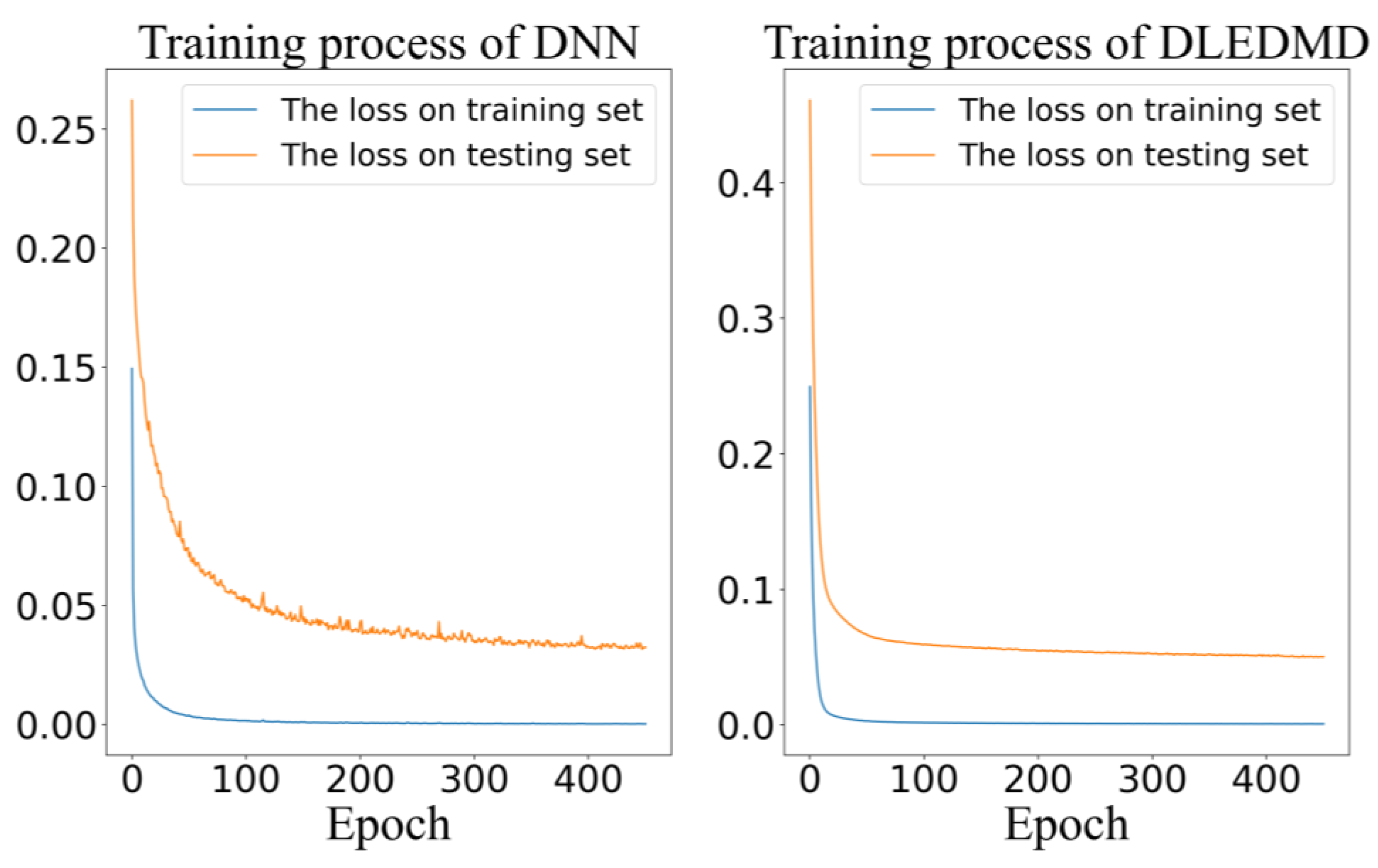
3.1. Training Process of DNN and DLEDMD

The loss function curves of DNN and DLEDMD during training process are shown in Figure 3. The training data consisted of randomly selected 1000 input–output pairs in the given time spans, and the validation data consisted of randomly selected 500 input–output pairs in the given time span. Each pair consisted of ${State}_t,{Control}_t,{Inflow}_t$, and ${Outflow}_{t+1}$. The training method and parameters were those provided in Section 2.2 and Section 2.3. From the training results, it is seen that both models progressively reduce their errors on the training set, demonstrating good training performance. They also show improvement on the testing set during the training process, indicating an increase in their generalization ability through training. However, DNN exhibits faster and better improvement on the testing set, suggesting that it has relatively better generalization ability compared to DLEDMD.

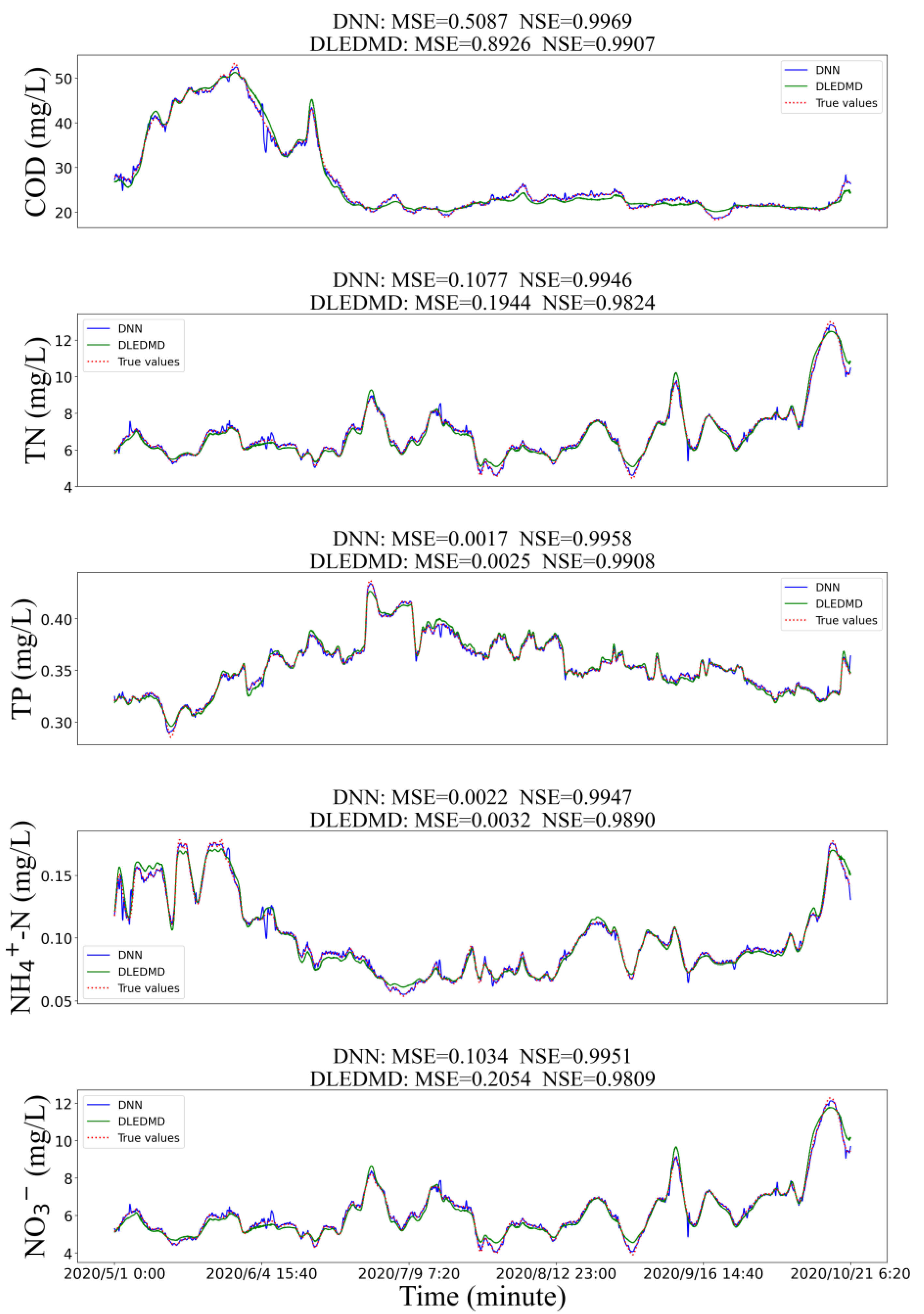
3.2. Simulation Performance

All the trained models were used to predict and simulate the outflow dynamic of A2O in the case study area. The predicted time ranged from 1 May 2020 at 0:00 to 21 October 2020 at 14:40. The models predicted the outflow in half an hour every 5 min, i.e., the time interval of prediction was half hourly and the frequency of prediction was 5 min, and there were a total of 49,901 predictions. The mean square error (MSE, Equation (15), where $Y_t$ is the output of models, $\overline{Y_{t+1}}$ is the true output values, $Num$ is the number of prediction, and is 49,901 in this study) and Nash–Sutcliffe efficiency coefficient (NSE, Equation (16), where $\mathbb{E}\left[\overline{Y_{t+1}}\right]$ is the mean value of true output values) were used to measure the performance of the two models.

$$MSE=\frac{1}{Num}\sum _{t=1}^{Num}{‖\overline{Y_{t+1}}-Y_{t+1}‖}^2$$

(15)

$$NSE=1-\frac{\sum _{t=1}^{Num}{‖\overline{Y_{t+1}}-Y_{t+1}‖}^2}{\sum _{t=1}^{Num}{‖\overline{Y_{t+1}}-\mathbb{E}\left[\overline{Y_{t+1}}\right]‖}^2}$$

(16)

The comparison between the predicted results of the two models and the actual values, as well as the MSE and NSE results, are shown in Figure 4. It can be seen from the figure that both data-driven models capture minor system disturbances and achieve good predictions with NSE reaching 0.99. At the same time, the comparison shows that the prediction performance of DLEDMD is slightly worse than that of DNN, which is consistent with the generalization performance in the training process of the two models.

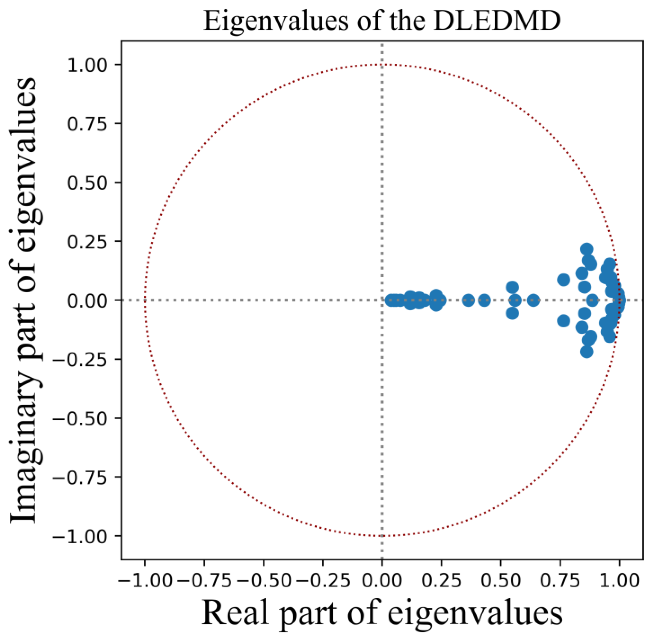
3.3. Eigenvalues of Koopman Matrix and Asymptotically Stablility of A2O Dynamic

Based on DLEDMD, we can directly obtain its corresponding Koopman matrix and use its eigenvalues to obtain the linearized description of the A2O nonlinear dynamical system through Equation (14). The eigenvalues of DLEDMD’s Koopman operator are shown in Figure 5. From the figure, it can be seen that the eigenvalues of the simulated dynamic of A2O process in this case study are all less than 1.

According to the Lyapunov stability theorem, a discrete time system such as DLEDMD in Equation (11) is asymptotically stable if and only if all its eigenvalues are inside the unit circle [16]. Therefore, the dynamic of the A2O in this case is asymptotically stable, and its output variables will gradually converge as the system runs without external influences. This means that the biochemical reactor in this case is capable of resisting fluctuations in influent water quality and control variables within a certain range. That is, the water quality of the effluent of the system will converge to a certain value and maintain stability when there is no continuous change in the influent water quality. Such a mathematical analysis can never be provided by DNN because the eigenvalues cannot be obtained from it.

4. Conclusions

Although data-driven methods have shown promise in the prediction of A2O dynamic in WWTPs, they cannot be helpful in the analysis of A2O dynamic properties. This study designed a data-driven prediction model using Koopman operators and deep learning methods to solve this problem. The method was validated using data from a real WWTP and compared to traditional deep learning methods. On the one hand, with the help of abundant data, this model accurately predicted the dynamics of the A2O process and captures small disturbances in practical situations. On the other hand, the Koopman operator was used to provide an analysis method for the dynamic properties of the A2O process from the perspective of mathematics.

Both DNN and DLEDMD learned the dynamics of the data through training and made relatively accurate predictions with NSE exceeding 0.99. However, according to the testing set error during the training process and the MSE and NSE values in the prediction, DNN had better generalization ability than DLEDMD because of its higher non-linearity. DLEDMD can be used to analyze the dynamic properties of the A2O process by utilizing its Koopman operator. In the case of this study, the trained DLEDMD directly obtained the Koopman matrix and its corresponding eigenvalues. The obtained eigenvalues indicates that the nonlinear dynamic system of A2O process in this study was Lyapunov asymptotic stable. This proves that the state and the effluent of the system will not undergo significant changes within a certain range of influent water quality disturbance in this case study. Moreover, when there is no sustained change in the influent water quality, the effluent quality of the A2O process will converge to a certain value and remain stable.

References

1. Chen, K.; Wang, H.; Valverde-Pérez, B.; Zhai, S.; Vezzaro, L.; Wang, A. Optimal control towards sustainable wastewater treatment plants based on multi-agent reinforcement learning. Chemosphere 2021, 279, 130498. [Google Scholar] [CrossRef] [PubMed]
2. Holenda, B.; Domokos, E.; Rédey, A.; Fazakas, J. Dissolved oxygen control of the activated sludge wastewater treatment process using model predictive control. Comput. Chem. Eng. 2008, 32, 1270–1278. [Google Scholar] [CrossRef]
3. Liu, X.; Jing, Y.; Xu, J.; Zhang, S. Ammonia Control of a Wastewater Treatment Process Using Model Predictive Control. In Proceedings of the 26th Chinese Control and Decision Conference (2014 CCDC), Changsha, China, 31 May–2 June 2014; pp. 494–498. [Google Scholar]
4. Elawwad, A.; Zaghloul, M.; Abdel-Halim, H. Simulation of municipal-industrial full scale WWTP in an arid climate by application of ASM3. J. Water Reuse Desalin. 2016, 7, 37–44. [Google Scholar] [CrossRef]
5. Henze, M.; Gujer, W.; Mino, T.; van Loosdrecht, M. Activated Sludge Models ASM1, ASM2, ASM2d and ASM3; IWA Publishing: London, UK, 2000. [Google Scholar]
6. Mulas, M.; Tronci, S.; Corona, F.; Haimi, H.; Lindell, P.; Heinonen, M.; Vahala, R.; Baratti, R. Predictive control of an activated sludge process: An application to the Viikinmäki wastewater treatment plant. J. Process. Control. 2015, 35, 89–100. [Google Scholar] [CrossRef]
7. Guo, H.; Jeong, K.; Lim, J.; Jo, J.; Kim, Y.M.; Park, J.-P.; Kim, J.H.; Cho, K.H. Prediction of effluent concentration in a wastewater treatment plant using machine learning models. J. Environ. Sci. 2015, 32, 90–101. [Google Scholar] [CrossRef] [PubMed]
8. Antwi, P.; Zhang, D.; Xiao, L.; Kabutey, F.T.; Quashie, F.K.; Luo, W.; Meng, J.; Li, J. Modeling the performance of Single-stage Nitrogen removal using Anammox and Partial nitritation (SNAP) process with backpropagation neural network and response surface methodology. Sci. Total. Environ. 2019, 690, 108–120. [Google Scholar] [CrossRef]
9. Khatri, N.; Khatri, K.K.; Sharma, A. Prediction of effluent quality in ICEAS-sequential batch reactor using feedforward artificial neural network. Water Sci. Technol. 2019, 80, 213–222. [Google Scholar] [CrossRef]
10. Hansen, L.D.; Stokholm-Bjerregaard, M.; Durdevic, P. Modeling phosphorous dynamics in a wastewater treatment process using Bayesian optimized LSTM. Comput. Chem. Eng. 2022, 160, 107738. [Google Scholar] [CrossRef]
11. Liu, H.; Wang, Y.; Fan, W.; Liu, X.; Li, Y.; Jain, S.; Liu, Y.; Jain, A.K.; Tang, J. Trustworthy AI: A Computational Perspective. ACM Trans. Intell. Syst. Technol. 2022, 14, 4. [Google Scholar] [CrossRef]
12. Samek, W.; Montavon, G.; Lapuschkin, S.; Anders, C.J.; Muller, K.-R. Explaining Deep Neural Networks and Beyond: A Review of Methods and Applications. Proc. IEEE 2021, 109, 247–278. [Google Scholar] [CrossRef]
13. Anders, C.J.; Weber, L.; Neumann, D.; Samek, W.; Müller, K.-R.; Lapuschkin, S. Finding and removing Clever Hans: Using explanation methods to debug and improve deep models. Inf. Fusion 2022, 77, 261–295. [Google Scholar] [CrossRef]
14. Fu, G.; Jin, Y.; Sun, S.; Yuan, Z.; Butler, D. The role of deep learning in urban water management: A critical review. Water Res. 2022, 223, 118973. [Google Scholar] [CrossRef]
15. Kozlov, V.; Furta, S. Lyapunov’s first method for strongly non-linear systems. J. Appl. Math. Mech. 1996, 60, 7–18. [Google Scholar] [CrossRef]
16. Datta, B.N. Chapter 7—Stability, inertia, and robust stability. In Numerical Methods for Linear Control Systems; Datta, B.N., Ed.; Academic Press: Cambridge, MA, USA, 2004; pp. 201–243. [Google Scholar]
17. De Santis, E.; Di Benedetto, M.; Pola, G. Stabilizability of linear switching systems. Nonlinear Anal. Hybrid Syst. 2008, 2, 750–764. [Google Scholar] [CrossRef]
18. Tu, J.H.; Rowley, C.W.; Luchtenburg, D.M.; Brunton, S.L.; Kutz, J.N. On dynamic mode decomposition: Theory and applications. J. Comput. Dyn. 2014, 1, 391–421. [Google Scholar] [CrossRef]
19. Mardt, A.; Pasquali, L.; Wu, H.; Noé, F. VAMPnets for deep learning of molecular kinetics. Nat. Commun. 2018, 9, 5. [Google Scholar] [CrossRef] [PubMed]
20. Montavon, G.; Lapuschkin, S.; Binder, A.; Samek, W.; Müller, K.-R. Explaining nonlinear classification decisions with deep Taylor decomposition. Pattern Recognit. 2017, 65, 211–222. [Google Scholar] [CrossRef]
21. Zhang, Y.; Tino, P.; Leonardis, A.; Tang, K. A Survey on Neural Network Interpretability. IEEE Trans. Emerg. Top. Comput. Intell. 2021, 5, 726–742. [Google Scholar] [CrossRef]
22. Budišić, M.; Mohr, R.M.; Mezić, I. Applied Koopmanism. Chaos Interdiscip. J. Nonlinear Sci. 2012, 22, 047510. [Google Scholar] [CrossRef]
23. Williams, M.O.; Rowley, C.W.; Mezić, I.; Kevrekidis, I.G. Data fusion via intrinsic dynamic variables: An application of data-driven Koopman spectral analysis. Europhys. Lett. 2015, 109, 40007. [Google Scholar] [CrossRef]
24. Bistrian, D.A.; Navon, I.M. An improved algorithm for the shallow water equations model reduction: Dynamic Mode Decomposition vs Pod: An Improved Algorithm for Dynamic Mode Decomposition vs Pod. Int. J. Numer. Methods Fluids 2015, 78, 552–580. [Google Scholar] [CrossRef]
25. Bistrian, D.A.; Navon, I.M. The method of dynamic mode decomposition in shallow water and a swirling flow problem: The Dmd Method in Shallow Water and a Swirling Flow Problem. Int. J. Numer. Methods Fluids 2017, 83, 73–89. [Google Scholar] [CrossRef]
26. Korda, M.; Mezić, I. Linear predictors for nonlinear dynamical systems: Koopman operator meets model predictive control. Automatica 2018, 93, 149–160. [Google Scholar] [CrossRef]
27. Han, Y.; Hao, W.; Vaidya, U. Deep Learning of Koopman Representation for Control. In Proceedings of the 2020 59th IEEE Conference on Decision and Control (CDC), Jeju Island, Republic of Korea, 14–18 December 2020; pp. 1890–1895. [Google Scholar]
28. Son, S.H.; Choi, H.-K.; Moon, J.; Kwon, J.S.-I. Hybrid Koopman model predictive control of nonlinear systems using multiple EDMD models: An application to a batch pulp digester with feed fluctuation. Control. Eng. Pract. 2021, 118, 104956. [Google Scholar] [CrossRef]
29. Page, J.; Kerswell, R.R. Koopman analysis of Burgers equation. Phys. Rev. Fluids 2018, 3, 071901. [Google Scholar] [CrossRef]
30. Klus, S.; Nüske, F.; Koltai, P.; Wu, H.; Kevrekidis, I.; Schütte, C.; Noé, F. Data-Driven Model Reduction and Transfer Operator Approximation. J. Nonlinear Sci. 2018, 28, 985–1010. [Google Scholar] [CrossRef]
31. Tian, W.; Wu, H. Kernel Embedding Based Variational Approach for Low-Dimensional Approximation of Dynamical Systems. Comput. Methods Appl. Math. 2021, 21, 635–659. [Google Scholar] [CrossRef]
32. Williams, M.O.; Kevrekidis, I.G.; Rowley, C.W. A Data-Driven Approximation of the Koopman Operator: Extending Dynamic Mode Decomposition. J. Nonlinear Sci. 2015, 25, 1307–1346. [Google Scholar] [CrossRef]
33. Felix, D.; Dietrich, F.; Bollt, E.M.; Kevrekidis, I.G. Extended dynamic mode decomposition with dictionary learning: A data-driven adaptive spectral decomposition of the Koopman operator. Chaos Interdiscip. J. Nonlinear Sci. 2017, 27, 103111. [Google Scholar]
34. Tian, W.; Liao, Z.; Zhang, Z.; Wu, H.; Xin, K. Flooding and Overflow Mitigation Using Deep Reinforcement Learning Based on Koopman Operator of Urban Drainage Systems. Water Resour. Res. 2022, 58, e2021WR030939. [Google Scholar] [CrossRef]
35. Sengupta, S.; Nawaz, T.; Beaudry, J. Nitrogen and Phosphorus Recovery from Wastewater. Curr. Pollut. Rep. 2015, 1, 155–166. [Google Scholar] [CrossRef]
36. LeCun, Y.; Bengio, Y.; Hinton, G. Deep learning. Nature 2015, 521, 436–444. [Google Scholar] [CrossRef] [PubMed]
37. Peitz, S.; Klus, S. Koopman operator-based model reduction for switched-system control of PDEs. Automatica 2019, 106, 184–191. [Google Scholar] [CrossRef]
38. Junge, O.; Koltai, P. Discretization of the Frobenius–Perron Operator Using a Sparse Haar Tensor Basis: The Sparse Ulam Method. SIAM J. Numer. Anal. 2009, 47, 3464–3485. [Google Scholar] [CrossRef]
39. Kingma, D.P.; Ba, J. Adam: A Method for Stochastic Optimization. arXiv 2014, arXiv:1412.6980. [Google Scholar]
40. Wu, H.; Noé, F. Variational Approach for Learning Markov Processes from Time Series Data. J. Nonlinear Sci. 2019, 30, 23–66. [Google Scholar] [CrossRef]
Figure 1. Architecture of DNN. The input of the DNN consists of S t a t e t , C o n t r o l t , I n f l o w t . Then, it goes through three separate deep neural networks and a combined layer for embedding and combination. The final output or result O u t f l o w t + 1 is calculated by the final deep neural network for simulation and prediction purposes.
Water 15 01960 g001
Figure 2. Architecture of DLEDMD. The input of the DLEDMD consists of S t a t e t , C o n t r o l t , I n f l o w t . Then, it goes through three separate deep neural networks and a combined layer for embedding and combination. This part is the ϕ in Equations (12)–(14). All the inputs and their combination are used to obtain the Koopman matrix. This is the only difference between DNN and DLEDMD. The final output or result O u t f l o w t + 1 is calculated by the final deep neural network for simulation and prediction purposes.
Water 15 01960 g002
Figure 3. Train process.
Water 15 01960 g003
Figure 4. Simulation results of DNN and DLEDMD.
Water 15 01960 g004
Figure 5. Eigenvalues of DLEDMD. Each blue point represents an eigenvalue, which is a complex number with both imaginary and real parts.
Water 15 01960 g005