1. Introduction
Water scarcity is considered a serious issue facing many countries worldwide, particularly arid and semi-arid countries such as those in the Middle East and North Africa (MENA) [
1,
2]. However, not only have arid and semi-arid regions recently faced water shortage problems, but also humid and Mediterranean regions, such as some European countries as a result of global climate changes [
3]. The demand for water resources is increasing because of population growth and agricultural expansion in addition to the rising municipal and industrial development [
3,
4,
5]. Based on data from the United Nations Food and Agriculture Organization (FAO), the agriculture sector accounts for about 70% of water consumption, followed by 20% for the industrial sector and 10% for the municipal [
6]. The gap between water demand and water supply has increased drastically, while global water demand is estimated to grow by almost 55% in 2050 [
6,
7]. From previous datasets of the water-consuming sectors, water recycling in the agricultural sector (i.e., the agricultural drainage and runoff water), which is subsequently used for irrigation [
8], is more economical than that in other sectors [
6].
Compared with groundwater, open water streams are generally more susceptible to pollution owing to the forthright discharge of untreated agricultural, municipal, and industrial wastewater [
9]. Furthermore, the absence of sanitation plants, particularly in developing countries, drives farmers to discharge untreated wastewater directly into the open agricultural drains [
10,
11]. Consequently, severe pollution of the water has occurred [
12]. Because of water scarcity from various causes, such as global climate change and constructing dams through transboundary rivers such as the Great Ethiopian Renaissance dam [
1,
6], the agricultural drainage water is generally reutilized [
8]. However, it is one of the most important non-point sources of water pollution, mainly because of the wide use of fertilizers, herbicides, and pesticides, so it is considered a main carrier of contaminants that will be reused in the agriculture sector [
13]; hence, the quality of water must be improved to meet the required international standard for limiting the environmental spread of contaminants [
11].
There are different technologies used to eliminate/degrade fertilizers, herbicides, and pesticides, such as biological, chemical, and physical processes [
11,
14]. The development of green technologies for the protection of environmental and human health is essential to minimize the contamination of natural water resources [
15]. Sorption and biodegradation are the main processes used to remove organic and inorganic contaminants from aqueous solutions [
16,
17,
18,
19].
The bioreactor is considered one of the most efficient technologies because it merges the sorption and biodegradation processes to enhance self-purification and improve water quality from an environmental and economic standpoint [
20]. Many studies have been conducted to investigate bioreactor media, and they have focused on the effects of different media on the efficiency of the removal of different contaminants from water bodies. Few studies have investigated the hydraulic impacts [
14,
15,
21,
22,
23,
24].
Although plenty of studies have dealt with bioreactors, there is a lack of studies dealing with the triggered hydraulic impacts. Bioreactors can be treated as porous media; thus, studies such as [
25,
26,
27] can be adopted to predict the hydraulic characteristics of stream flow where they are installed. El-Saiad et al. [
11] investigated the hydraulic characteristics of flow induced by installing a bioreactor inside an open channel. The impact of flow rate and water depth, in addition to different specifications of the bioreactor regarding the relative heading up, was experimentally investigated [
6,
11]. The key objective of this study is to investigate numerically the hydraulic impacts of different arrangements (i.e., divisions and inclination) of bioreactors installed on an open channel. The relative heading up was also investigated under different Froude’s numbers representing the actual domain of different drains. This study is uniquely focused on passing the entire discharge of the open drains through the bioreactor, where the previous studies dealt with a submerged bioreactor, in which part of the discharge flows through the submerged bioreactor and the other part flows over the submerged bioreactor.
2. Methodology and Numerical Modeling
2.1. Methodology
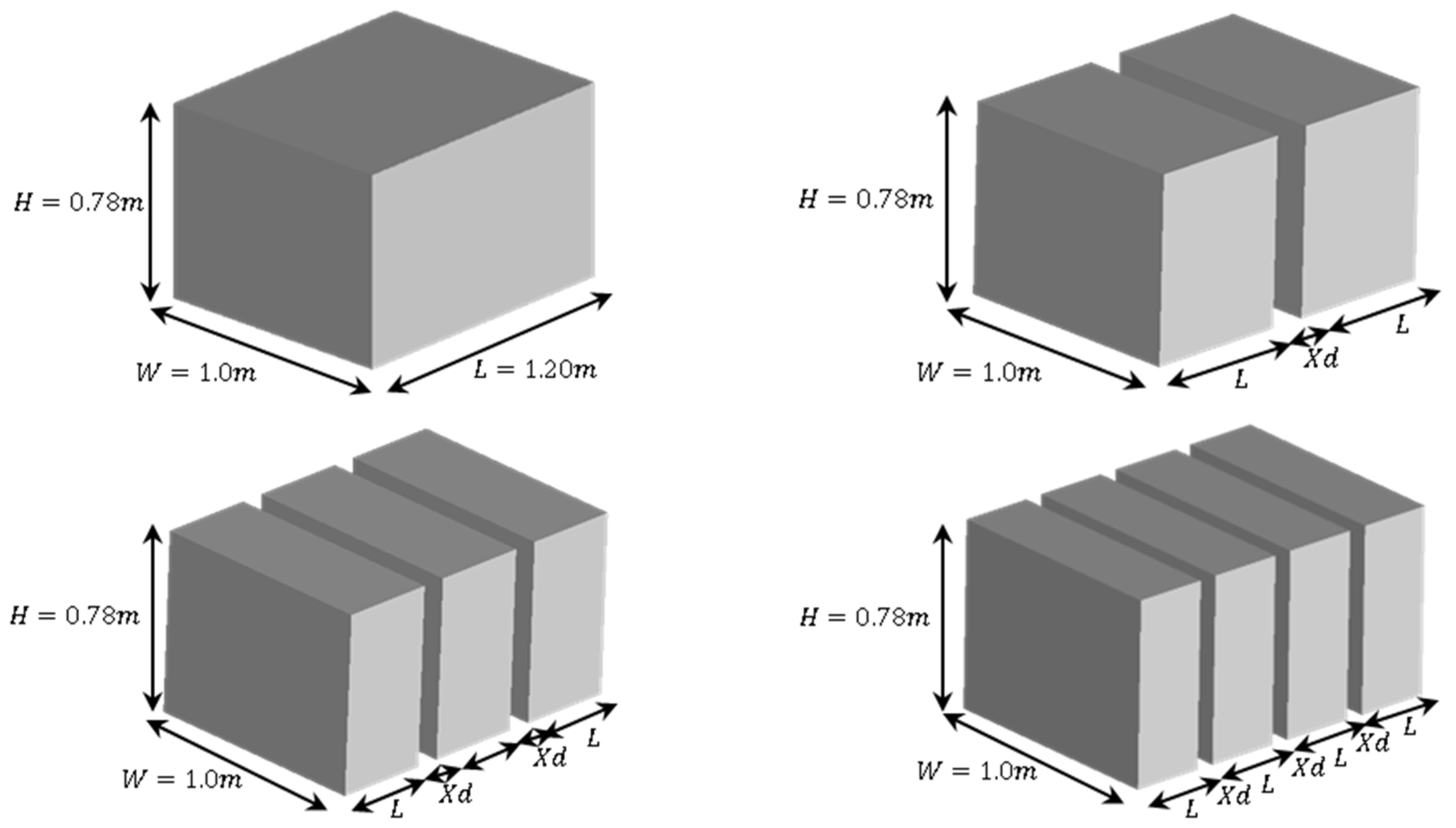
This study was conducted to numerically simulate gravel bio-filters under different conditions, to examine their resulting hydraulic impacts on the watercourses, and to understand and mitigate these impacts. The different studied scenarios were as follows: the first scenario studied different discharges and therefore different velocities, and consequently different Froude’s numbers representing the actual domain of drains. The second scenario was based on using a fixed length of bio-filter equal to 1.20 m. In this scenario, the fixed length was divided into several segments, where the sum of the total lengths of the segments remained 1.20 m. The impact of the distance between the segments of the bio-filter was also investigated. In other words, the second scenario investigated the effect of both the length of the bio-filter segments and their inter-spacing on the triggered heading up. The third scenario dealt with different inclination angles of the bio-filter to examine their impacts on the induced heading up, considering four angles: 45°, 60°, 75°, and 90°.
The numerical model dimensions were the following. In the X-direction, the total length of the model was 10.0 m. The mesh block consisted of four mesh planes that were adjusted at distances of 0.0, 4.40, 5.60, and 10.0 m with a uniform cell size of 0.035 m. In the Y-direction, the total width of the model was 1.0 m. The mesh block consisted of two mesh planes that were adjusted at distances of 0.0 and 1.0 m with a uniform cell size of 0.035 m. In the Z-direction, the total height of the model was 1.0 m. The mesh block consisted of four mesh planes that were adjusted at distances of 0.0, 0.60 (i.e., initial water depth), 0.78 (i.e., bio-filter height), and 1.0 m with a uniform cell size of 0.035 m.
2.2. Relevant Theory
The numerical simulation was conducted using powerful computational fluid dynamics (CFD) FLOW-3D software [
28]. The bio-filter geometry was prepared by a CAD program in a stereolithographic (STL) format as shown in
Figure 1. The stereolithographic (STL) file was then imported to FLOW-3D, after which the numerical simulations were begun. Reynolds-averaged Navier–Stokes equations (RANS) were employed as governing equations for the flow in the three dimensions, as indicated in Equations (1) and (2). In FLOW-3D, the governing equation (i.e., Reynolds-averaged Navier–Stokes) is solved by using the finite volume method (FVM). The finite volume method is an Eulerian method for describing, analyzing, and converting partial differential equations to algebraic equations [
29], where values are obtained at discrete nodes in the mesh geometry. In this technique, the divergence theorem is utilized to transform volume integrals containing a divergence term into surface integrals, where finite volume describes a small volume surrounding each node point on a mesh. These terms are then assessed as fluxes at the surfaces of each finite volume.
The momentum equation:
where
is time-averaged velocity,
is kinematic viscosity,
is fractional volume open to flow,
is averaged pressure, and
are components of Reynold’s stress.
The free surface profile tracking process was achieved by the volume of fluid (VOF) algorithm proposed by Hirt et al. [
30]. The occupancy of a grid cell with fluid is presented by the function (F). The value of (F) ranges from zero to unity; the zero value denotes that there is no fluid present in the grid cell, while the unity value denotes that the fluid completely fills the grid cell. The free surface forms for grid cells with (F) values between zero and unity are indicated by Equation (3).
where (u, v, w) are the velocity components in (x, y, z) coordinates, respectively, and (A
x, A
y, A
z) are the area fractions.
2.3. Boundary and Initial Conditions
To increase the accuracy of the numerical model results, the boundary conditions should be carefully defined. To minimize the simulation time, one mesh block was used. The mesh block boundary conditions in the three directions were as follows: In the X-direction, X
min (i.e., inlet) was defined as volume flow rate and X
max (i.e., outlet) was defined as a specified pressure with 0.6 m fluid elevation. In the Y-direction, Y
min and Y
max were defined as a wall. In the Z-direction, Z
min was defined as a wall and Z
max was defined as a specified pressure with assigned atm pressure as shown in
Figure 2. The initial conditions of the numerical model included the following: configuration, temperature, velocity, and pressure distribution. The configuration of the fluid was determined by the shape and dimensions of the waterway. While the temperature was assigned as 25 °C, the initial velocity was assigned as 0.0 m/s, and the pressure distribution was assigned as hydrostatic pressure.
2.4. Grid Type and Time Step
Simple rectangular orthogonal elements in planes and hexahedral elements in volumes were used in FLOW-3D to simplify mesh generation, reduce memory requirements, and increase numerical accuracy. A grid convergence test was used to determine the optimum mesh size to ensure the results of the numerical model were accurate and efficient. According to the grid convergence test, the mesh block cell size was 0.035 m. A Courant number was used to determine the maximum time-step size. This number controls the distance that the flow can moves in each time step during the simulation. To avoid the flow passing through more than one cell in a time step, the Courant number in this work was set equal to 0.25. The maximum time step value was 0.00075 s, according to the Courant number.
2.5. Turbulent and Porous Media Models
Fluids move chaotically and unstably when there are not enough stabilizing viscous forces, and this is known as turbulence. The two-equation (k − ε) model, the two-equation (k − ω) models, and the renormalization-group (RNG) model are among the most widely applied models of turbulence behavior within FLOW-3D. The RNG model is used to represent flow motion because it simulates motion behavior better than the (k − ε) and (k − ω) models [
31]. The turbulent kinetic energy
and its dissipation
are the main equations in the RNG model, as expressed in Equations (4) and (5), respectively:
where
is the turbulent kinetic energy,
is the turbulent kinetic energy production,
is the buoyancy turbulence energy,
is the turbulent energy dissipation rate,
and
are terms of diffusion,
,
and
are dimensionless parameters, in which
and
have constant values of 1.42 and 0.2, respectively,
is computed from the turbulent kinetic energy (
) and turbulent production (
) terms.
The porous media model is used to compute the drag and capillary pressure effects in porous media such as soils, fractured rock, sponges, and paper. Porous media refers to solid materials with connected interstitial voids through which fluid can flow. The porous media model is appropriate when the size of the pores is much smaller than the size of the control volume, such as sandstone and gravel. The porosity of a porous medium is defined as the open volume divided by the total volume. In FLOW-3D nomenclature, porosity is identical to volume fraction
as expressed in Equation (6).
Materials such as metallic foam filters are almost completely open and may have porosities approaching 1.0. While the porosity of close-packed spheres (i.e., gravel) varies from 25% to 47% depending on the packing configuration, the porosity of the gravel bio-filter used in this study was 39%. The usual conservation equations were obtained by constructing a continuum model of the porous material and applying averaging to each control volume. Conservation of mass is expressed by Equation (7):
where
is the fluid density and
is the microscopic flow velocity.
The momentum equation in porous media can be formed based on the observation of Henry Darcy in 1856, who noted that the unidirectional flow rate through porous media is proportional to the applied pressure difference. This relationship is expressed in Equation (8):
where
is the coefficient of permeability of the material and
is dynamic viscosity.
Values of
for common materials are (10
−7–10
−9) m
2 for gravel and (10
−13–10
−16) m
2 for clay. The smaller the value of permeability, the greater is the resistance to flow. This resistance is commonly referred to in porous media modeling as drag. The resistance to flow in a porous medium is represented in the Navier–Stokes equations as a drag term proportional to the velocity, as indicated in Equation (9):
where
is the porous media drag coefficient.
When the porous medium is composed of coarse particles or fibers, the microscopic velocity may be significant, and the flow losses it induces may be proportional to the square of the flow velocity as well as being a linear function of the velocity. In Forchheimer’s equation, the pressure drop is given by Equation (10):
where
is the non-Darcian or inertial permeability. The linear Darcian and quadratic non-Darcian flow loss equations can be combined into a single expression for
indicated in Equation (11):
where
are constant coefficients,
is the Reynolds number, and
is the particle diameter.
3. Numerical Modeling Validation
To adjust the numerical model accuracy, a comparison was made between the numerical model results and the experimental work presented by El-Saiad et al. [
11]. The experimental study of El-Saiad et al. [
11] used a star-shaped media with 87% porosity and 1.20 m in length, and the relative heading up (hup/H) was 10.25%. While, in this study, the used media was gravel with a porosity of 39%, and the relative heading up was found 4.10%. Although El-Saiad et al. [
11] used a media with porosity higher than that used in this study; the induced relative heading up was low. This can be attributed to the orientation of the media with respect to the flow direction, as shown in
Figure 3. In which, in this study, the arrangements of the gravel voids were uniform, regardless of the flow direction. While, in El-Saiad et al. [
11], it was found that the plastic star-shaped voids arrangement was significantly depended on the flow direction. Consequently, the orientation of the bio-filter media plays a significant role in the induced heading up values.
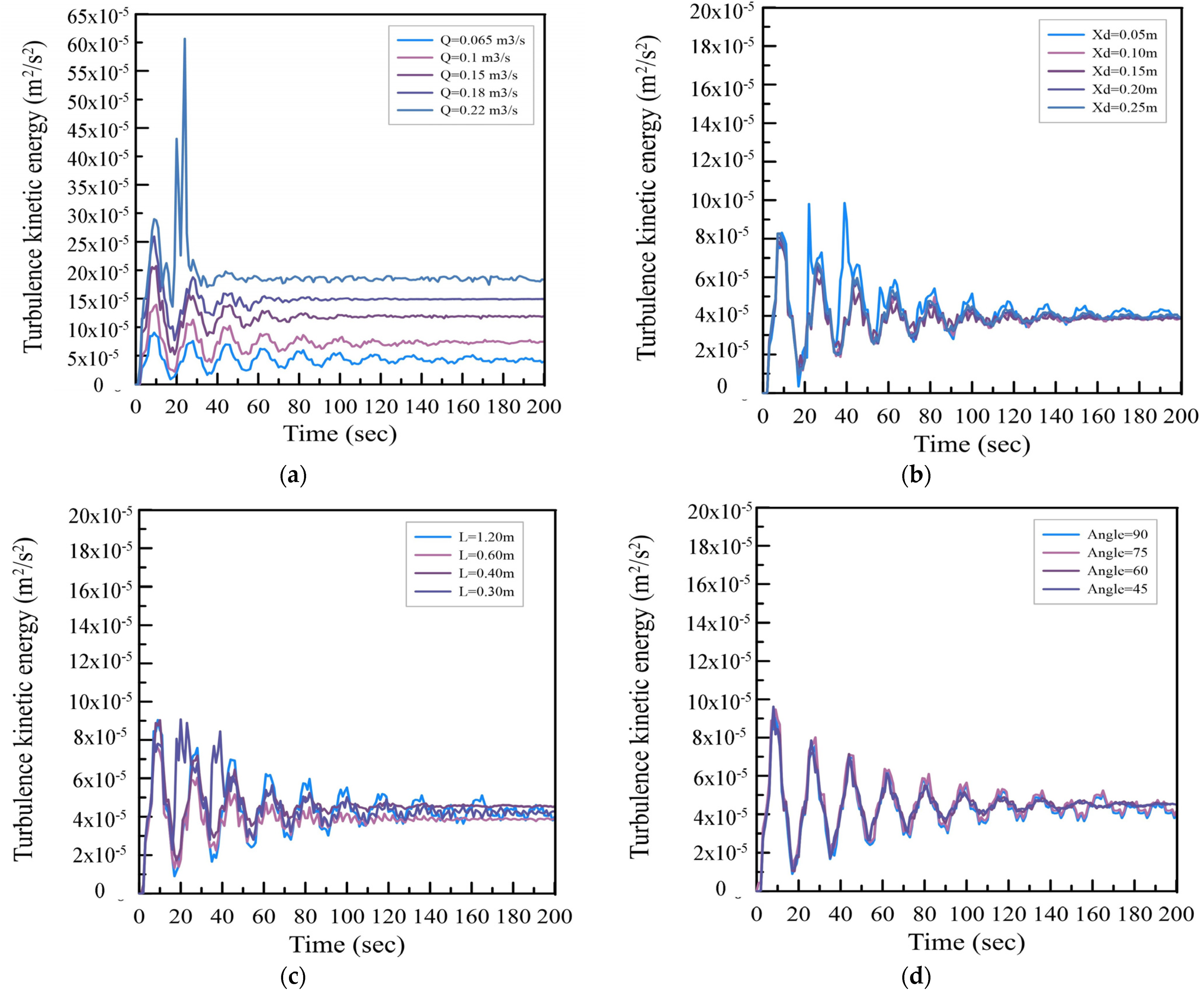
Figure 4 shows the turbulence kinetic energy versus time, it is clear that the chosen time domain (i.e., 200 s) was suitable to reach the steady state for different discharges and different conditions of bio-filters (i.e., length, distances, and angles).
4. Results and Discussion
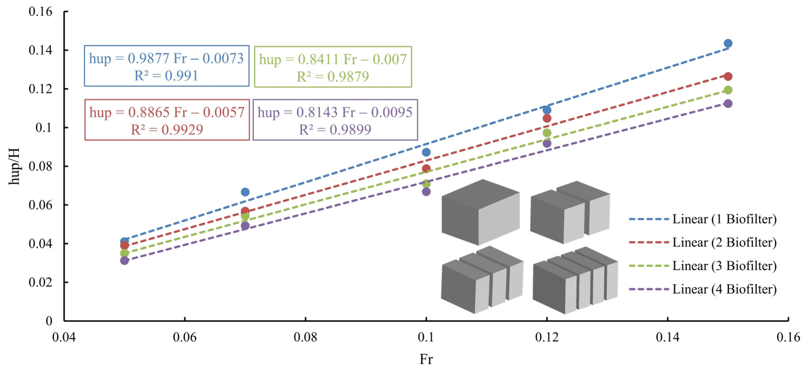
Figure 5 shows the relation between the relative heading up (hup/H) and Froude’s number for different segmented bio-filters having the same total length of 1.20 m when investigating the effect of discharge and velocity on the heading up. As expected, the relative heading up increased as the Froude’s number increased, regardless of the number of segments, where a linear direct proportionality was found for all bio-filter arrangements. This can be attributed to the increase in velocity, where the bio-filter represented an obstacle that suddenly existed in the water flow path and in turn reduced the speed of water flow through it. Consequently, the heading up formed, and as the flow velocity increased, the accumulation of water in front the bio-filter increased. Froude’s number was also in a direct proportionality with flow velocity, thus the heading up increased as the Froude’s number increased. In other words, as the discharge increased, the velocity increased and consequently, Froude’s number, eventually leading to increasing the relative heading up. It was also clear that when at the same value as Froude’s number, the relative heading up of one segment’s bio-filter at 1.20 m in length had the highest value of heading up. The value of the relative heading up decreased significantly after dividing the bio-filter into several segments with the same total length (i.e., the one-segment bio-filter was 1.20 m in length, the two-segment was 2 × 0.60 m in length, the three-segment was 3 × 0.40 m in length, and the four-segment was 4 × 0.30 m in length). For example, at a Froude’s number of 0.15, the relative heading up values were 0.1123, 0.1194, 0.1263, and 0.1435, corresponding to bio-filters of four segments, three segments, two segments, and one segment, respectively. The rate of increase in the relative heading up was 6.25% when using three segments instead of four segments. When using two segments rather than four segments the rate of increase was 12.46%, and when using one segment rather than four segments the increase ratio was 27.77%. It could be concluded that dividing the bio-filter into several segments was hydraulically better than using one segment having the same length.
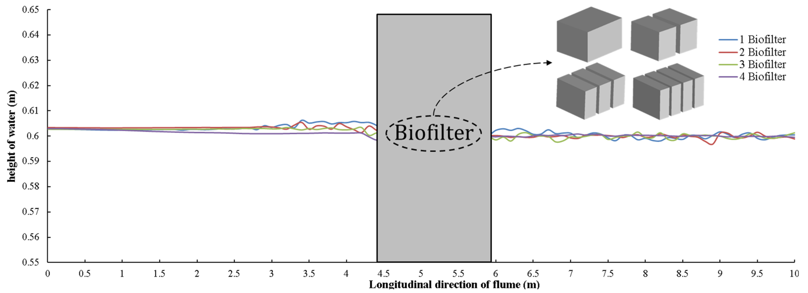
Figure 6 shows the water surface profiles of different bio-filters, and it is obvious that the one-segment bio-filter had the highest value of heading up, followed by the two-segments, then the three-segments, and finally the four-segments bio-filter had the lowest value of heading up, which confirmed the previously mentioned observation. It can be also noticed that the heading up vanished at a distance of nearly 4.0 m, which represents about 3.3 the length of the used bio-filter.
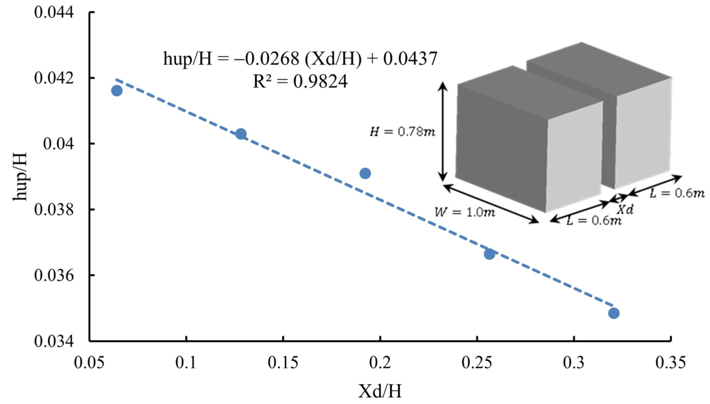
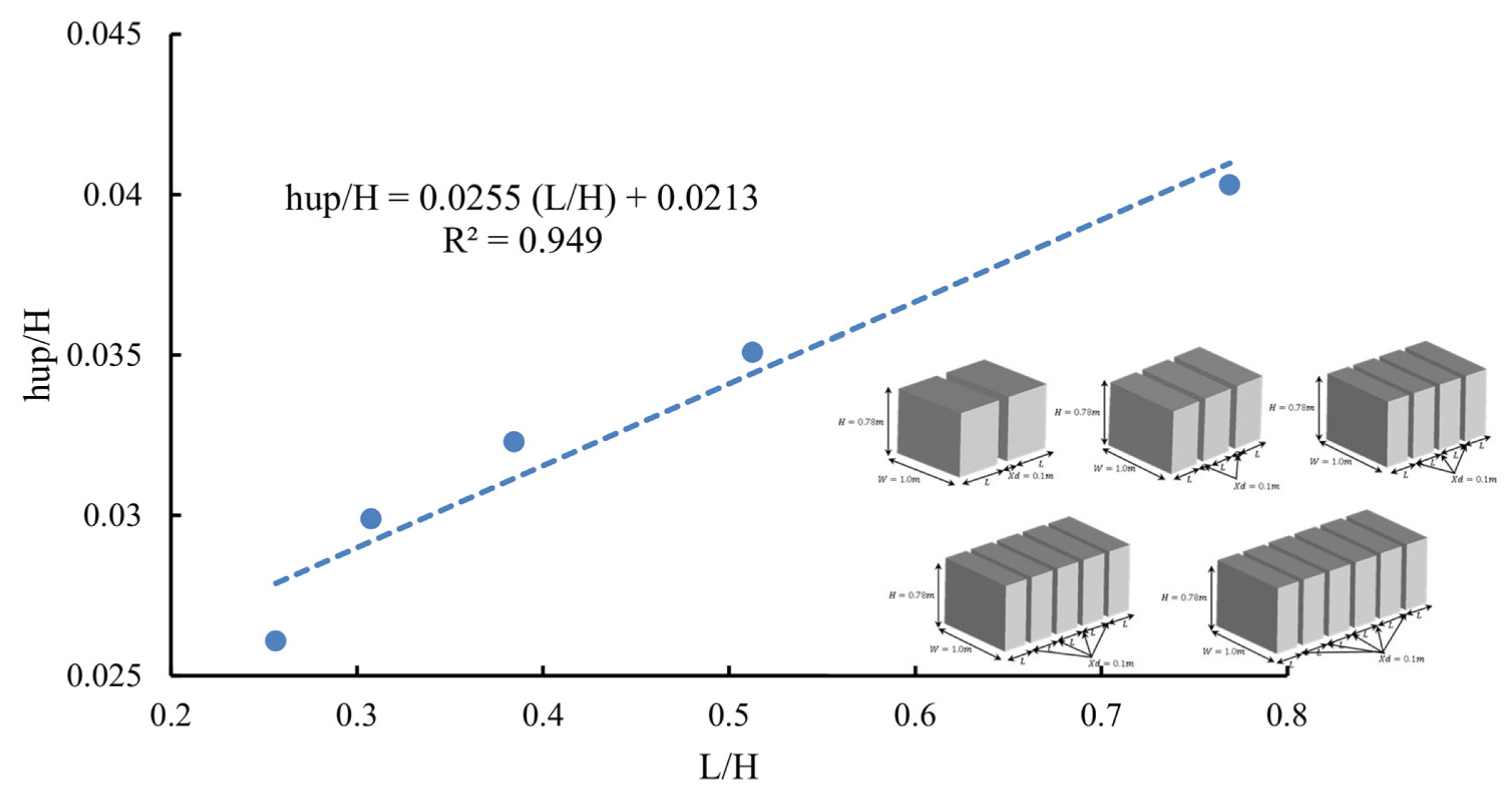
Figure 7 shows the relation between the relative heading up and the distance between two segments of the bio-filter with the same total length of 1.20 m (i.e., the length of each segment was 0.60 m) at the same Froude’s number. The relative heading up decreased linearly as the distance (Xd) between the two bio-filter segments increased. On the other hand,
Figure 8 shows the relative heading up versus the length of the segments at the same bio-filter length of 1.2 m, with a constant distance between the segments equal to 10 cm. The relative heading up increased linearly as the length of the bio-filter segments increased. This can be explained by the following: increasing the length of the bio-filter segment leads to decreasing the velocity through it, based on Darcy’s law of flow through porous media. Where velocity is in direct proportionality with the hydraulic gradient, and the hydraulic gradient is reversely proportional with the length, the velocity through the bio-filter’s segment is reversely proportional with the length as a consequence. Therefore, increasing the bio-filter segment length means an increase in the obstacle’s length, which in turn means an increase in the triggered heading-up values.
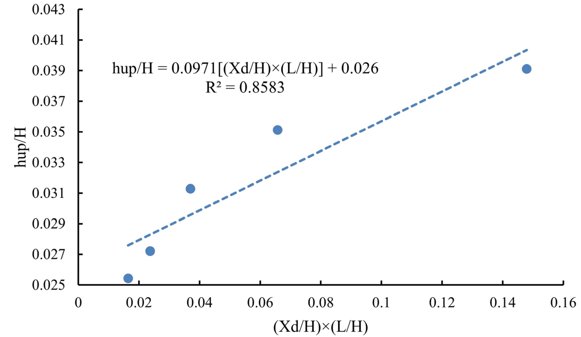
To shed more light on the simultaneous change in both the length of the bio-filter’s segments and their inter-distance, additional simulations were conducted as indicated in
Table 1. It can be clearly seen from
Figure 9 that the relative heading up increased when increasing the product of both the length and inter-distance of the bio-filter (i.e., the value of (Xd/H) × (L/H)). This means that increasing the length of the bio-filter’s segment on the induced relative heading up had a greater effect than increasing the distance between the bio-filter segments. Therefore, the relative heading up increased with the product of the length and inter-distance of the bio-filter. However, the rate of increase in the relative heading up decreased as the values of the product of (Xd/H) × (L/H) increased; thus, the value of R
2 was almost 0.85. The regression analysis technique was used to produce the relationship between the relative heading up and the simultaneous change in both the bio-filter’s length and the inter-distance. It was found that the relation produced from regression analysis was more accurate than the relation that correlates between the relative heading up and (Xd/H) × (L/H), where the R
2 was 0.96 and significance = 0.0076. The actual values of the relative heading up produced from the numerical simulation were close to the values produced from the regression analysis, as indicated in
Table 2.
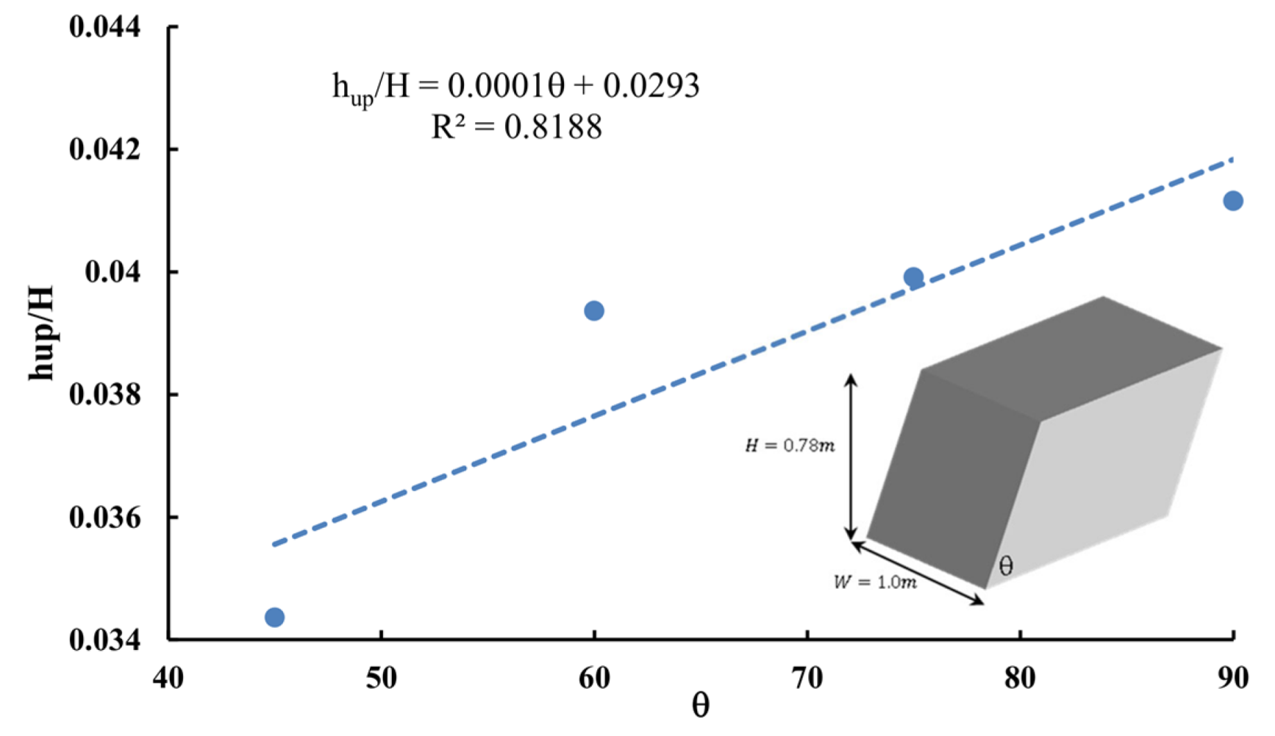
Figure 10 depicts the relation between the inclination angles of the bio-filter and the relative heading up; in this study four different angles were investigated. It can be clearly seen that the greater the inclination angle, the greater the heading up. The 90° angle showed the highest relative heading up value, followed by 75°, 60°, and finally 45°. This can be imputed to the area of the inclined bio-filter face, where the length of the inclined face of the bio-filter increased as the inclination angle decreased [
32,
33]. However, the rate of increase in the relative heading up values decreased as the inclination angle increased, in which the relative heading up values were 0.0343, 0.0391, 0.0399, and 0.041 corresponding to the angles 45°, 60°, 75°, and 90°, respectively. This means that by considering the base case where the inclination angle is 45°, the increasing ratios of the relative heading up were 14.5%, 16.1%, and 19.7% corresponding to the angles 60°, 75°, and 90°, respectively.
5. Conclusions
Recently, unconventional water resources management has become an urgent need because of global climate change and erection of dams through transboundary rivers. Recycling the agricultural drainage water is considered an effective policy to meet the demand–supply gap in regions that suffer from a scarcity of water resources. The agricultural drains are contaminated with different pollutants; thus, water cannot be used directly and requires treatment to meet the international standards before utilizing. A bioreactor is considered an effective approach to enhancing the self-purification of the agricultural drains when considering the hydraulic impacts. The results showed that the relative heading up increased as the Froude’s number increased, regardless of the number of bio-filter segments. This means that the greater the increase in velocity and discharge of flow, the greater the increase in the relative heading up. The value of heading up decreased significantly by dividing the bio-filter into several segments with the same total length. The increase rates in the relative heading up values were 27.77%, 12.46%, and 6.25% when using one, two, and three segments, respectively, instead of four segments, which confirmed that dividing the bio-filter into several segments was hydraulically better than using one segment having the same length. The relative heading up decreased linearly as the distance (Xd) between bio-filter segments increased for a constant length of bio-filter. However, the relative heading up increased linearly as the length of the bio-filter segments increased for a constant inter-distance of the bio-filter’s segments. For the simultaneous change in both the bio-filter segments’ length and their inter distance, the relative heading up increased with the product of the length and inter-distance of the bio-filter. This means that the effect of increasing the length of the bio-filter’s segment on the induced relative heading up was higher than that of increasing the inter-distance of the bio-filter’s segments. The inclination angle of 90° showed the highest relative heading-up value, followed by the 75° angle, then the 60° angle, and finally the 45° angle. This can be imputed to the area of the inclined bio-filter face, where the length of the inclined face of the bio-filter increased as the inclination angle decreased. However, the rate of increase in the relative heading-up values decreased as the inclination angle increased. It can be concluded that the higher the inclination angle of the bio-filter’s face, the greater the heading up.


 ,
, 


