Article

Investigate the Difference of Cooling Effect between Water Bodies and Green Spaces: The Study of Fuzhou, China

1
College of Environment and Safety Engineering, Fuzhou University, Fuzhou 350108, China
2
Department of Environmental and Resources Engineering, Fuzhou University Zhicheng College, Fuzhou 350002, China
*
Author to whom correspondence should be addressed.
Water 2022, 14(9), 1471; https://doi.org/10.3390/w14091471
Submission received: 23 March 2022 / Revised: 20 April 2022 / Accepted: 27 April 2022 / Published: 4 May 2022

Abstract

:
The urban heat island (UHI) effect will persist for a long time and influence human health, energy consumption, and future urban planning. Understanding the cooling effect of water bodies and green spaces can help alleviate the frequency of extreme climate, especially during torridity seasons. In this study, correlation and regression analysis were used to measure the relationship between land surface temperature (LST) or cooling indicators and landscape factors. In addition, the cooling intensity, distance, and threshold value of efficiency (TVoE) of water bodies and green spaces were detected. The results confirmed that: first, the cooling effect of water bodies were stronger than that of vegetation in most cases and more water bodies’ layout in the region was advocated; second, increasing vegetation coverage within 27% of the region can effectively and economically alleviate the thermal environment; and third, the green samples with an area of 0.57 ha and a high vegetation index had a higher cost performance ratio. The results provided quantitative guidance for urban public service spatial planning of water bodies and green spaces to prevent the continuous increase of urban background temperature.

1. Introduction

As claimed in the Emissions Gap Report 2021 released by the United Nations Environment Programme (UNEP), the new and updated climate pledges submitted by countries fall far short of The Paris agreement’s temperature targets, which could result in an increase of 2.7 °C in the world’s average temperature by the end of the century [1]. In general, urban tends to have higher temperature than the surrounding countryside, which forms a condition similar to high-temperature islands. This phenomenon is defined as the urban heat island (UHI) effect [2]. The main reasons for the UHI effect can be divided into the following four categories: the increase of urban impervious surface, the decrease of natural underlying surface (green spaces, water bodies and croplands) and increasing overall heat emission; the anthropogenic heat emission increases significantly as the urban population gathers; the monolithic buildings in cities hinder airflow, reduce urban wind speed and aggravate UHI phenomenon; the increasing frequency and intensity of extreme weather events further aggravate the UHI effect [3,4,5]. Increasing urban temperature caused by the UHI effect will have an impact on ecology and the environment [6,7,8]. In terms of energy consumption, cooling buildings could consume an additional 8.5% of electricity for every degree increase in urban ambient temperature [9]. Besides, the frequent occurrence of extreme heat can increase morbidity, mortality, and health risks for urban dwellers [10,11,12]. Nearly half of the world’s poor are frequently affected by high temperatures, a number that is still rising fast [13]. The UHI effect will persist for a long time in numerous cities, which has become the major research direction of urban planning and needs to be solved urgently.
Numerous studies specialized in mitigating UHI effects with proven strategies [14,15,16,17]. In general, studies have illustrated that designing water bodies, increasing green spaces cover (lawn, forest, shrubbery), implementing a night ventilation strategy of chimney ventilation, and changing materials with high reflectivity on the impervious surface (roof, road) can mitigate UHI effectively [18,19,20,21,22]. Studies have shown that plants in green spaces can absorb surrounding heat through evapotranspiration, absorb carbon dioxide through photosynthesis, and shield solar radiation from the tree canopy which can significantly reduce temperature [23]. The green spaces often form low-temperature islands via reducing the temperature of the surrounding non-vegetation environment through airflow [24]. Meanwhile, Water bodies are a better radiation absorber than other urban underlying surface materials. Water bodies have a large heat capacity which allows them to absorb a great amount of heat; it provides efficient heat absorption by evaporating water bodies, and it takes advantage of short-wave radiation and can be transmitted to appropriate depths. For example, through a meta-analysis of the data of 27 meteorological stations in the city, the water bodies in the northern hemisphere can produce a cooling effect of 16.4 °C during the warmest months [25]. Many researchers believed that urban water bodies and green spaces were indispensable for local ecological environment protection and urban planning, and reasonable planning of them was the most economical and effective [26,27]. Hence, taking advantage of the cooling capacity and potential of water bodies and green spaces for the surrounding environment is increasingly regarded as a promising way to mitigate the UHI effect [28,29].
The majority of research explored the characteristics and dimensions of the UHI effect alleviated by water bodies and green spaces. Generally speaking, the amount (patch size and coverage) of water bodies and green spaces is positively correlated with the cooling effect it provides, but the amount is not the only influencing factor. Factors that characterize green spaces also influence cooling effects. For example, Peng [30] and Kuang [31] showed that the normalized vegetation index (NDVI) of green space increased, and the land surface temperature (LST) decreased. Besides, shape indicators also play a role in the cooling effect, but it is still controversial [32,33]. According to the study by Yu [32], circular or square green spaces had stronger cooling capacity. In addition, surrounding landscape composition will also affect the ability of water bodies and green spaces to alleviate the UHI effect. In recent research in Wuhan [22], when the lake was surrounded by compact midrise buildings, the lake could reduce the LST of the surrounding environment within the range of 1000 m, while the lake surrounded by the compact low-rise building region only provided the influence range of 300 m.
Various cooling indicators have been defined to quantify the ability of water bodies and green spaces to provide cooling effects to the urban thermal environment [34,35,36]. Recent research by Yu showed that the average cooling intensity of Beijing lakes in summer was 6.54 °C and the average cooling distance was 383.41 m, which represented the cooling effect and influence range that water bodies could provide for the surrounding environment [37]. In addition, in the context of rapid urbanization, it was impractical to increase the amount of water bodies and green spaces indefinitely [38,39]. Therefore, some studies proposed an indicator named Threshold Value of Efficiency (TVoE) [32] to quantitatively calculate the optimal area of water bodies and green spaces. Yu found that the TVoE of cities in Temperate monsoon and Mediterranean climates was generally around 0.5 ha [30]. The TVoE is a cost-effective cooling indicator that provides a quantitative reference for planning and may become one of the key solutions to balance urban modernization and urban ecological environment protection.
At present, mitigation of the UHI effect through water bodies and green spaces has become the focus of public attention, however, the research on how to plan and design water bodies and green spaces to alleviate the UHI effect is not specific. This study showed that the impact of water bodies and green spaces coverage rate and landscape (internal and external) factors on mitigation of UHI effect. To improve the efficiency of water bodies and green spaces in alleviating UHI effect, this study quantified the cooling indicators of water bodies and green spaces, and thus clarified the correlation between each factors and cooling indicators to obtain the optimal coverage range. Therefore, the UHI effect can be alleviated through the scientific design and planning of urban water bodies and green spaces, providing a scientific basis for the design of urban water bodies and green spaces in the future.

2. Materials and Methods
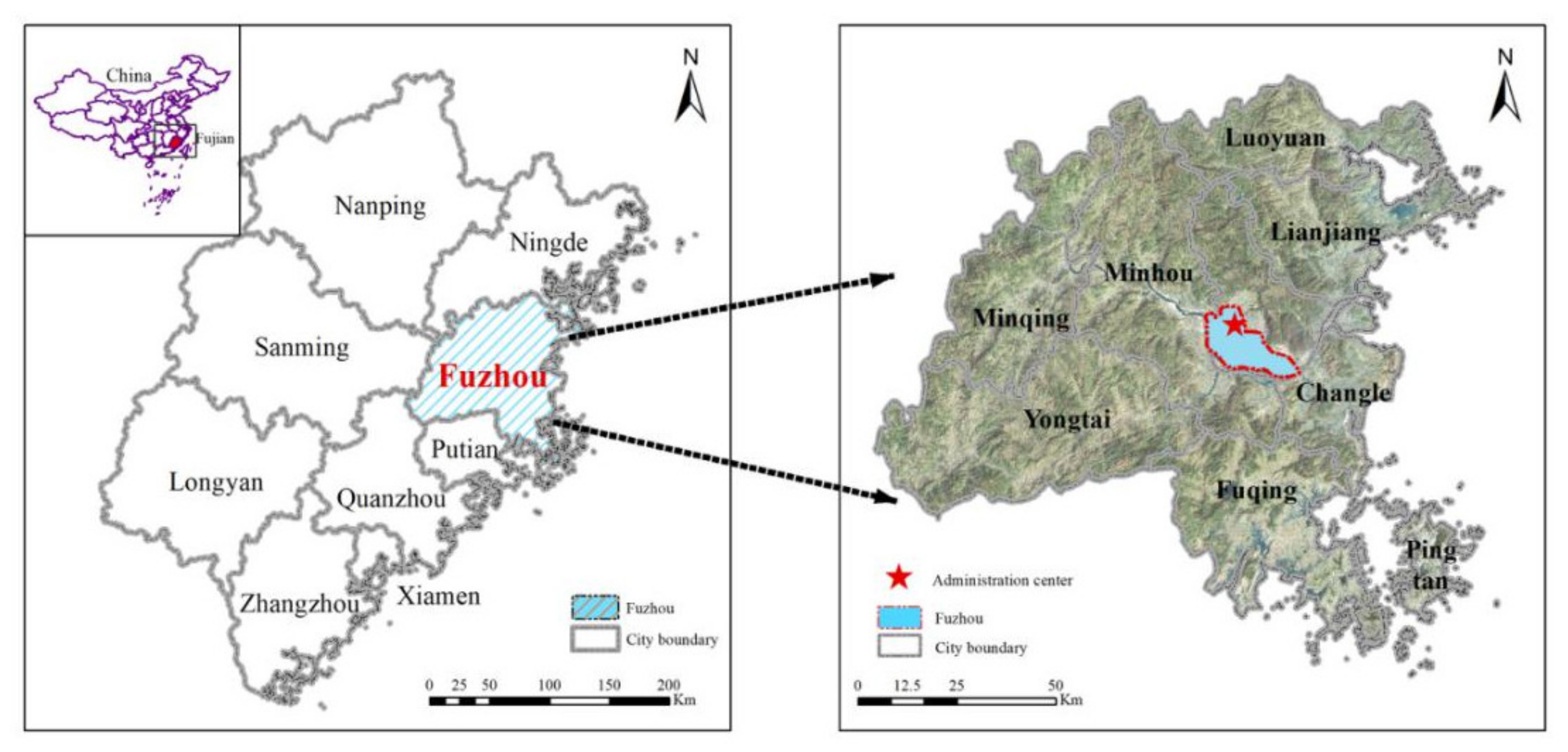
2.1. Study Region

Fuzhou (25°15′–26°39′ N, 118°08′–120°31′ E), locates in the lower reaches of the Minjiang River, east of the southeast Sea of China (Figure 1). Fuzhou is a subtropical monsoon city, summers are long, very hot, and humid, and winters are short and warm. In recent years, with the rapid development of urbanization, the urban underlying surface has changed dramatically, and the UHI effect becomes significant [40]. During of urbanization, LST increased 4–6 °C on average from 1989 to 2016 [41]. In 2020, number of days of high temperature (>35 °C) in Fuzhou reached 87 with 3 days of extreme heat (>40 °C). The city has become the hottest city in China, referred to as the “Furnace City”. Fuzhou has plentiful hydrological conditions [42,43]. As a typical city developed along the rivers, the mainstream of the Minjiang River is divided into north and south tributaries through the urban core regions. Meanwhile, there are dense inland river networks in the urban region. Besides, the green spaces of Fuzhou have been continuously eroded. The total area of green spaces stock decreased by 8.85% in 1986–2020, and the spatial distribution of green spaces are gradually fragmented. In order to mitigate the UHI effect and the impact of heat waves, as well as to improve the urban environment, the construction of water bodies and green spaces has become a very important policy for the Fuzhou municipal government.

2.2. Data Source

High-resolution remote sensing images with mildly atmospheric impact were derived from the websites (https://www.gscloud.cn) (accessed on 22 October 2021) of the Chinese Academy of Sciences, in order to obtain different landscape characteristics data and land surface temperature data over the years. Due to climate and research requirements, we selected Landsat images of 24 May 2010, 27 September 2015, 22 July 2020 with low cloud cover (0.34%, 1.76% and 11.77%, respectively), while the image cloud amount of 2020 is basically outside the study area. Besides, Google images with high-resolution and Open Street Map (https://www.openstreetmap.org/) (accessed on 30 October 2021) were used to extract water bodies and green spaces boundaries as a supplementary tool.

2.3. Data Processing

2.3.1. Retrieved of LST

Previous studies have generally adopted single-channel algorithms, split-window algorithm, and radiative transfer equation to retrieving LST. However, the radiative transfer equation was used to retrieve LST in the thermal infrared bands of Landsat-5 and Landsat-8 in this study. For Landsat-8, band10 and band11 are both thermal infrared bands [44]. According to Yu [39], LST accuracy based on the radiative transfer equation inversion of band-10 was higher than that of band-11. LST retrieval results from 2010 to 2020 were shown in Figure 2.

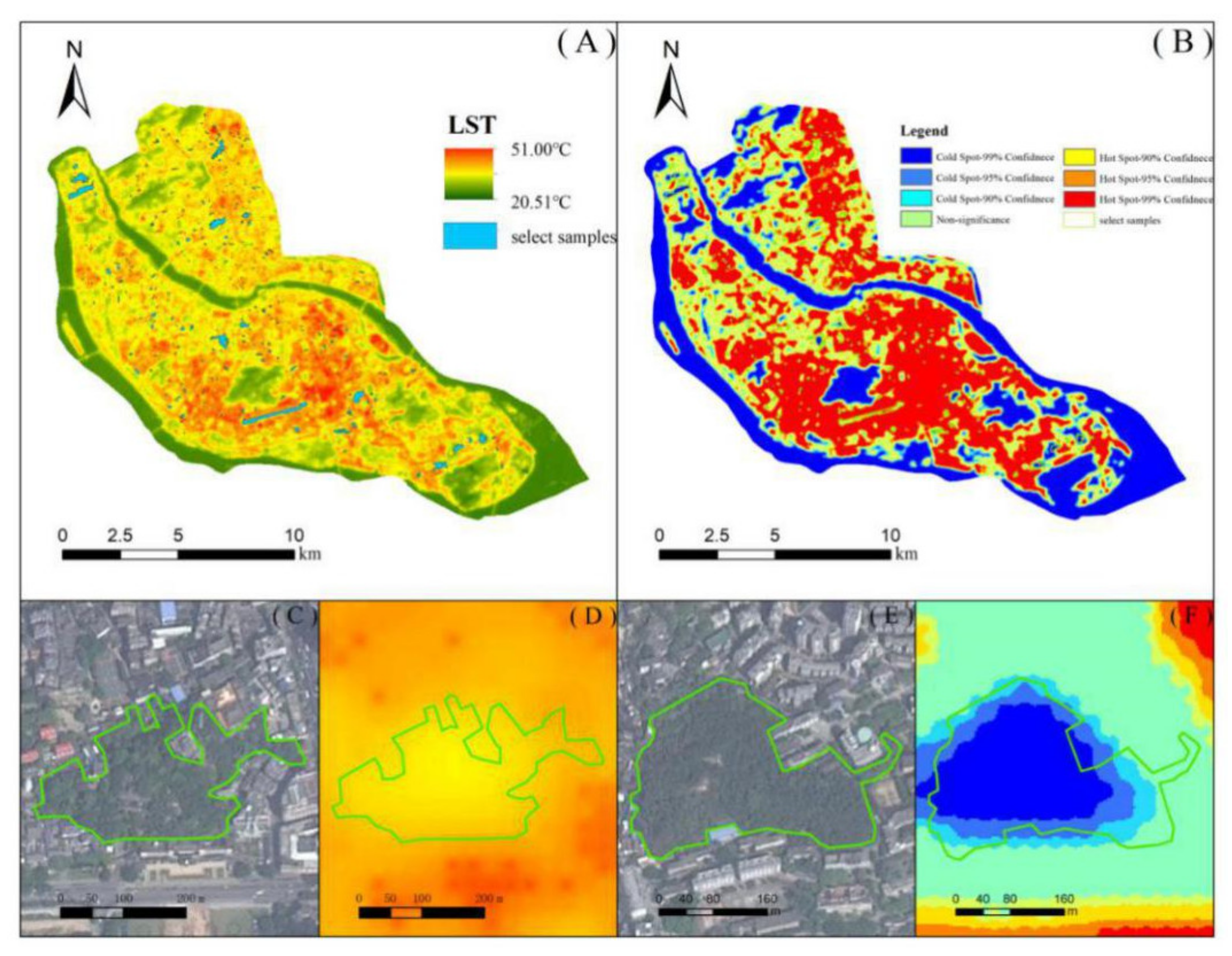
2.3.2. Extraction of Water Bodies and Green Spaces Samples

According to SAVI (The Soil Adjusted Vegetation Index) combined with high-resolution Google image, we extracted the urban green patch basis of different years in the study area. In low-vegetation areas such as urban built-up areas, the lower limit of SAVI’s detection vegetation coverage can be as low as 15%, which is better than NDVI’s 30% [45]. Based on Equation (1).
SAVI = [(NIR − Red)(1 + l)]/(NIR + Red + 1)
where, NIR and Red are reflectance of mid-infrared and visible Rad bands of OLI or TM+ respectively. L is the soil regulatory factor, and 0.5 is usually selected.
MNDWI (The Modified Normalized Difference Water Index) is widely used to extract urban water from remote sensing image and obtain its boundary [46,47], based on Equation (2).
MNDWI = (GREEN − MIR)/(GREEN + MIR))
Here, MIR and GREEN are reflectance of mid-infrared and visible Green bands of OLI or TM+ respectively. The usually threshold is 0. Water bodies are all grids with MNDWI value greater than 0 [47].
The resulting raster layer was converted into vector plane domain layer in ArcGIS and modified with high resolution image. The selection of green spaces samples and water samples should meet the following conditions: (1) the area range of green spaces patch was 0.09–40 ha; (2) to avoid the cooling effect caused by water bodies, selected patches should be more than 300 m away from water bodies; (3) to avoid the shadow of tall buildings affecting the LST results, the selected samples should be checked according to the high resolution image to see if there are some tall buildings around. According to the above rules, urban water bodies and green spaces samples selected in different years are represented in Figure 3.

2.4. Analytical Method and Measurement Indicators

2.4.1. Buffer Analysis

In order to explore quantitative indicators and the same method to measure the cooling effect of water bodies and green spaces, we built a series of buffer with a 30 m interval. For green spaces, 16 continuous buffers were created covering a range of 480 m, while 70 continuous buffers were created covering a range of 2100 m, the average LST in each buffer and the average LST in the sample can obtained. Besides, due to the LST was derived from 30 m retrieval remote sense images, there would be deviation between the average LST in the statistical sample and the buffers. To increase the continuity of LST with buffer, LST was interpolated from 30 m to 1 m by spline function.

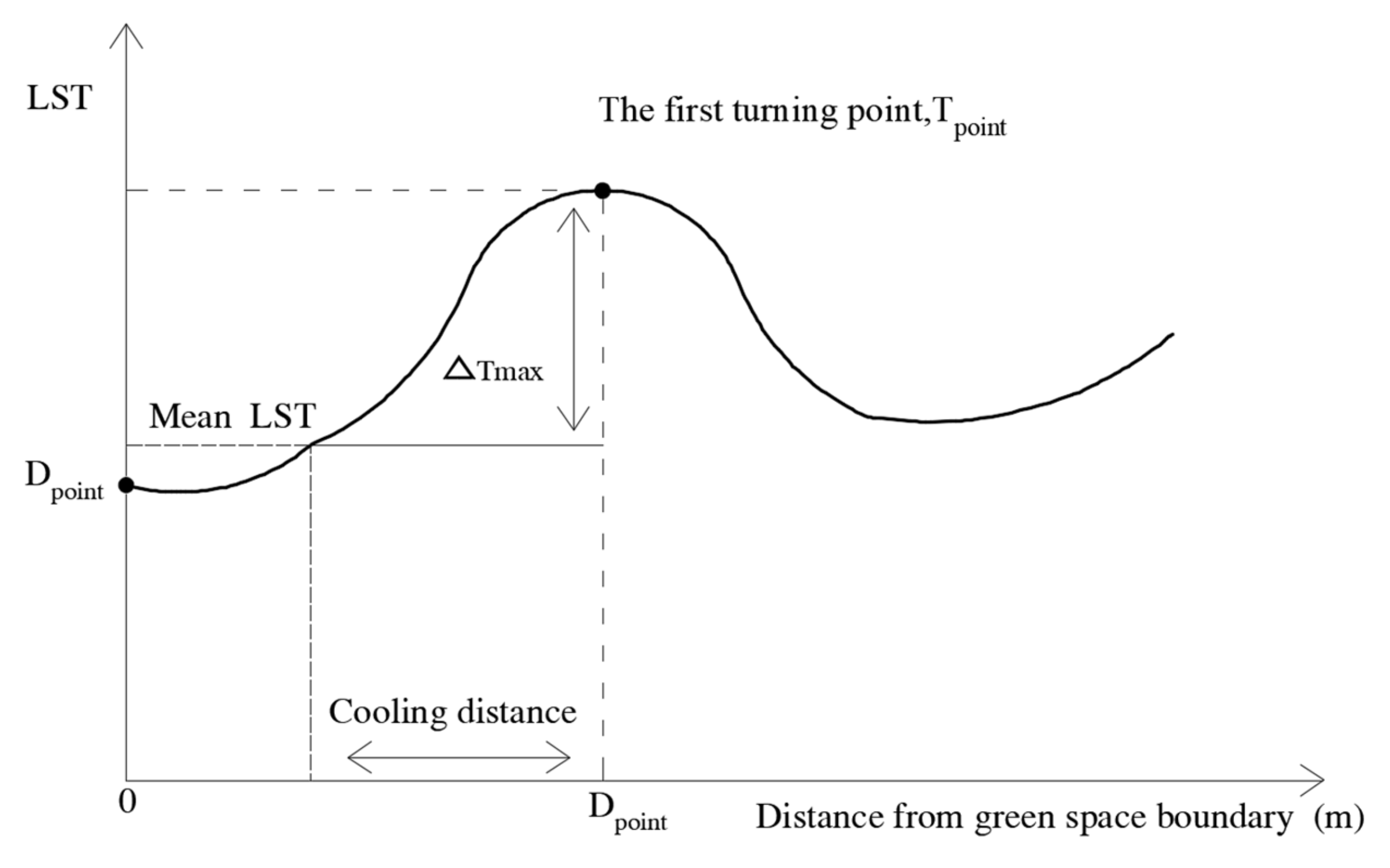
2.4.2. Description of Cooling Effect Indicators

To quantify the cooling effect of water bodies and green spaces, several cooling indicators were used to describe the cooling effect [48,49]. The maximum temperature difference (ΔTmax) between water bodies and green spaces and surrounding urban area was defined as the green spaces cooling intensity (GCI) and water bodies cooling intensity (WCI); in addition, the cooling distance (GCD and WCD, respectively) represents how far the cooling effect extends. The buffer distance was plotted as the X-axis, and the average LST of each buffer as the Y-axis. Different curve fitting analysis results showed that cubic polynomial was better than other fitting methods and can best describe the relationship. As shown in Figure 4, Tpoint was the turning point of the first decline, while the distance from samples border to Tpoint was Dpoint and the maximum temperature difference between the LST of Tpoint and mean LST of samples was recorded ΔTmax. Hence, when the Tpoint appeared, the value of ΔTmax as cooling intensity and Dpoint as cooling distance could be calculated.
Besides, previous studies have found that TVoE can be used to measure cooling efficiency. There was a logarithmic relationship between ΔTmax and sample area size, the curve showed that with the increase of sample area, ΔTmax also increased, however, the increase rate was gradually slowed down, until a certain point, ΔTmax will stabilize in a certain range, and the point is TVoE. In this study, when the slope of the fitted logarithmic curve was 1, the area value of the sample is TVoE [50].

2.4.3. Internal and External Impact Factors

Characteristics of area and shape were usually selected to figure out how they affect the cooling effect of water bodies and green spaces, but many uncertainties still remain. Here, the landscape factors were divided into internal and external factors to analyze what characteristics would affect the cooling effect and the degree of influence (Table 1). Internal factors referred to patch structure including area, landscape shape index (LSI), SAVI within the samples (SAVIinside), and fractal dimension index (FRAC), while the external factors were the composition of surrounding landscapes, including proportion of impervious surface (PI), and SAVI of the surrounding environment (SAVIoutside). Besides, vegetation and water coverage was used to measure the thermal environment of the region where people live.

3. Results

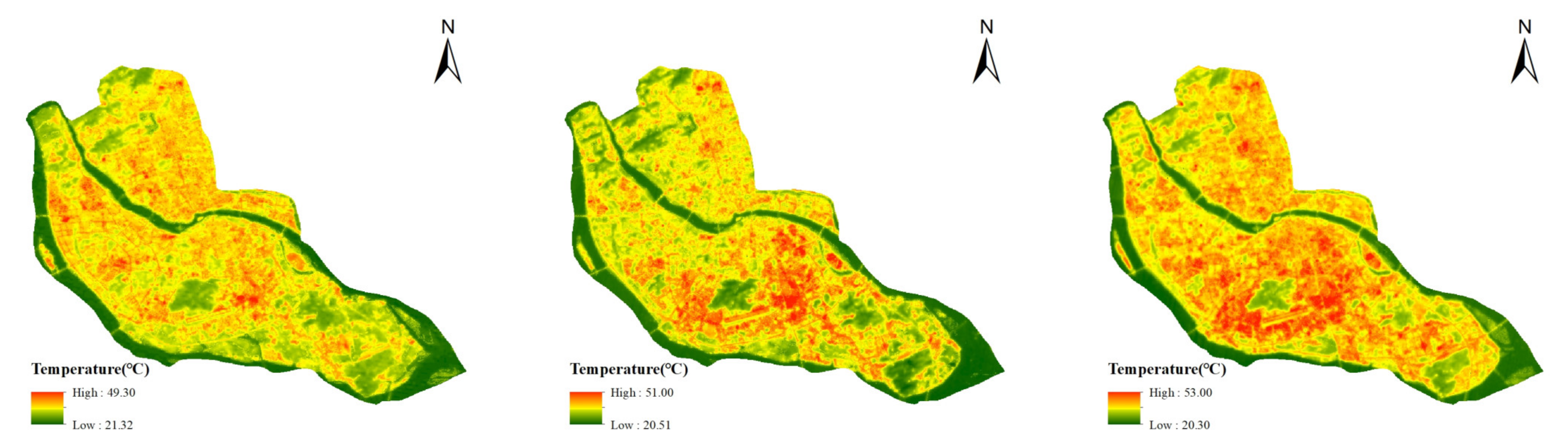
3.1. Analysis of LST

According to Table 2, the average LST in the study region on 22 July 2020 (40.92 °C) was higher than that on 24 May 2010 (32.65 °C) and 27 September 2015 (32.65 °C). The maximum value of LST was also increasing year by year, from 49.30 °C in 2010 to 53.00 °C in 20 years. As shown in Figure 5A, the phenomenon of UHI was obvious in the study region. The impervious surface composed of buildings such as commercial regions, industrial regions, residential regions, construction sites to be built and roads had produced different degrees and scales of heat concentration. At the same time, there were also some regions with obvious low-temperature aggregation phenomena, such as rivers (Minjiang River), forests, lakes (West Lake) and urban inland rivers. These areas were water bodies or large-scale green spaces with an area larger than 40 ha. According to the research of the cooling effect of green spaces, take Yushan Scenic Area, a famous park in Fuzhou as an example in Figure 5C,D. The highest average temperature in the green spaces in three years was 41.85 °C (2020) and the lowest average temperature was 32.48 °C (2010). The maximum temperature difference with the surrounding environment was 4.01 °C (2010) and the minimum was 2.45 °C (2015).
Hot spot analysis method judged the hot spots and cold spots in the whole study region by studying a neighboring numerical value, and the hot spots (cold spots) were often the aggregation of multiple high-value points (low-value points). In order to better reflect the distribution of LST in time and space, the hot spot analysis method was used to measure the spatial location where high-temperature (low-temperature) aggregation occurred and the degree of high-temperature (low-temperature) aggregation. In Figure 5B, the blue regions were cold spots, meant that the region in the study region was low temperature, whereas the hot spot meant that the region was high temperature. The three-year average green spaces coverage of cold spots (90–99% confidence) reached 63.45%, and the three-year average water bodies’ coverage of cold spots (90–99% confidence) reached 98.16%. Most of the green patches in the electoral districts of Figure 5E, F are cold spots (99% confidence), the surrounding environment was the hot spots with increasing confidence (90–99% confidence) were distributed on the periphery. When studying the temperature difference between green patches and the surrounding environment, only 4.1% of the samples showed that the average green temperature was lower than the surrounding temperature. The above conclusions indicated that water bodies and green spaces would produce certain cold spots in the urban thermal environment and had a cooling effect on the ambient temperature.

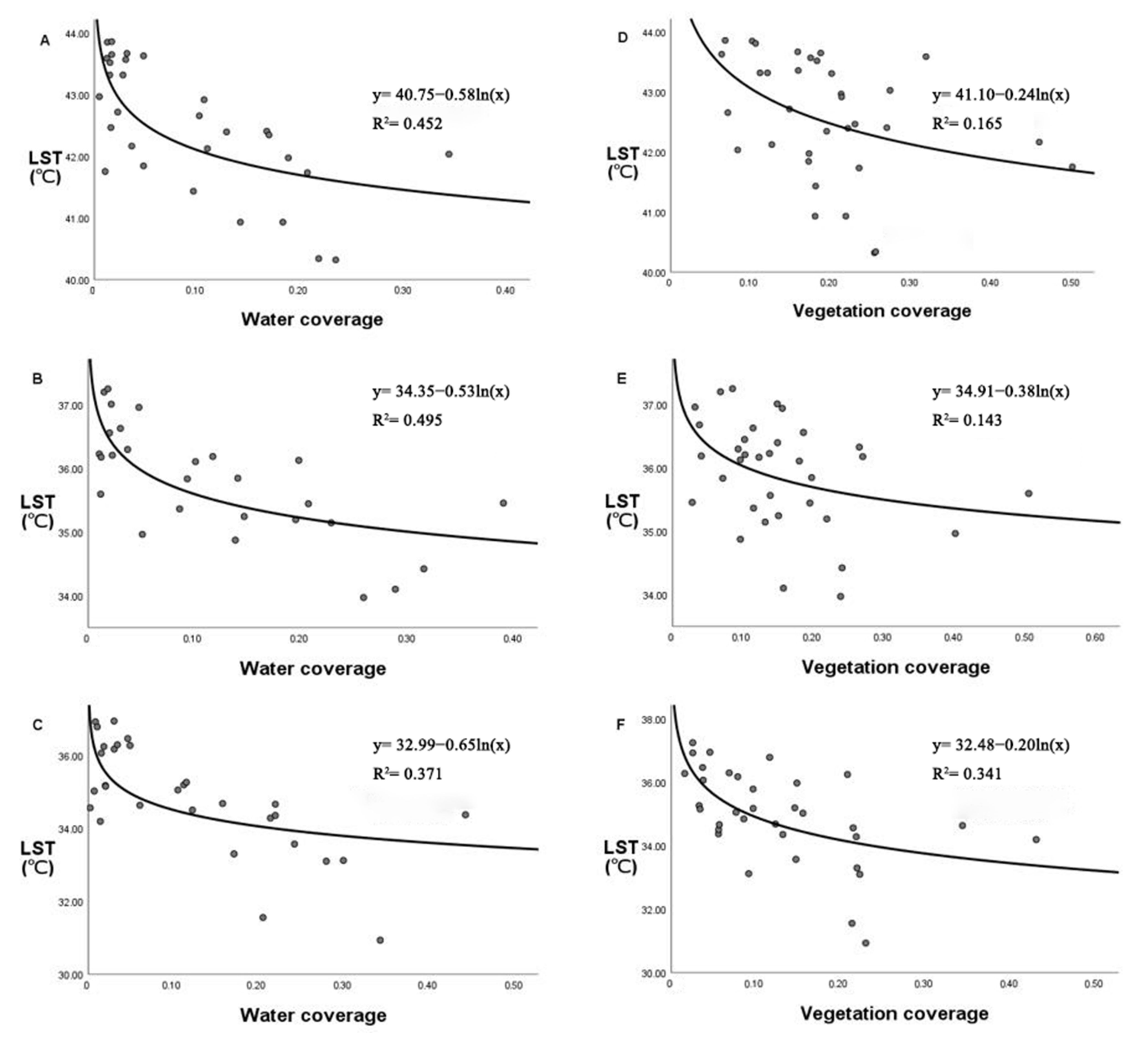
3.2. Relationships between LST and Vegetation and Water Coverage

There are 34 streets with different vegetation and water coverage under three administrative districts in the study area. According to the results of Pearson correlation analysis (Table 3), from 2010 to 2020, the LST and water coverage of each street in Fuzhou were negatively correlated, respectively −0.708, −0.722 and −0.721, with an average correlation of −0.717. Similar results were found for vegetation coverage, which were −0.360, −0.366, and −0.519, respectively, with an average correlation of −0.415. The correlation between LST and water coverage was more significant than that between vegetation coverage, indicating that increasing water coverage in the study area was more effective than increasing vegetation to reduce air temperature.
The result showed that the logarithmic relationship best describes the relationship between region coverage and LST (Figure 6). The turning point was defined as the point at which the slope of the logarithm function was 1. Before the turning points, LST declined rapidly as the vegetation and water coverage increases; as such, increasing coverage before turning points was cost-effective. From 2010 to 2020, the water coverage at turning points was 65%, 53% and 58%, respectively, and the average value was 58%. Therefore, increasing water coverage within the range of 0–58% can effectively reduce the LST in the region. Similarly, the vegetation values at the turning point from 2010 to 2020 were 24%, 38% and 24% respectively, and the average value was 27%. Increasing vegetation coverage within 27% of the region can effectively and economically alleviate the thermal environment.

3.3. Cooling Effect Measured by Different Indicators

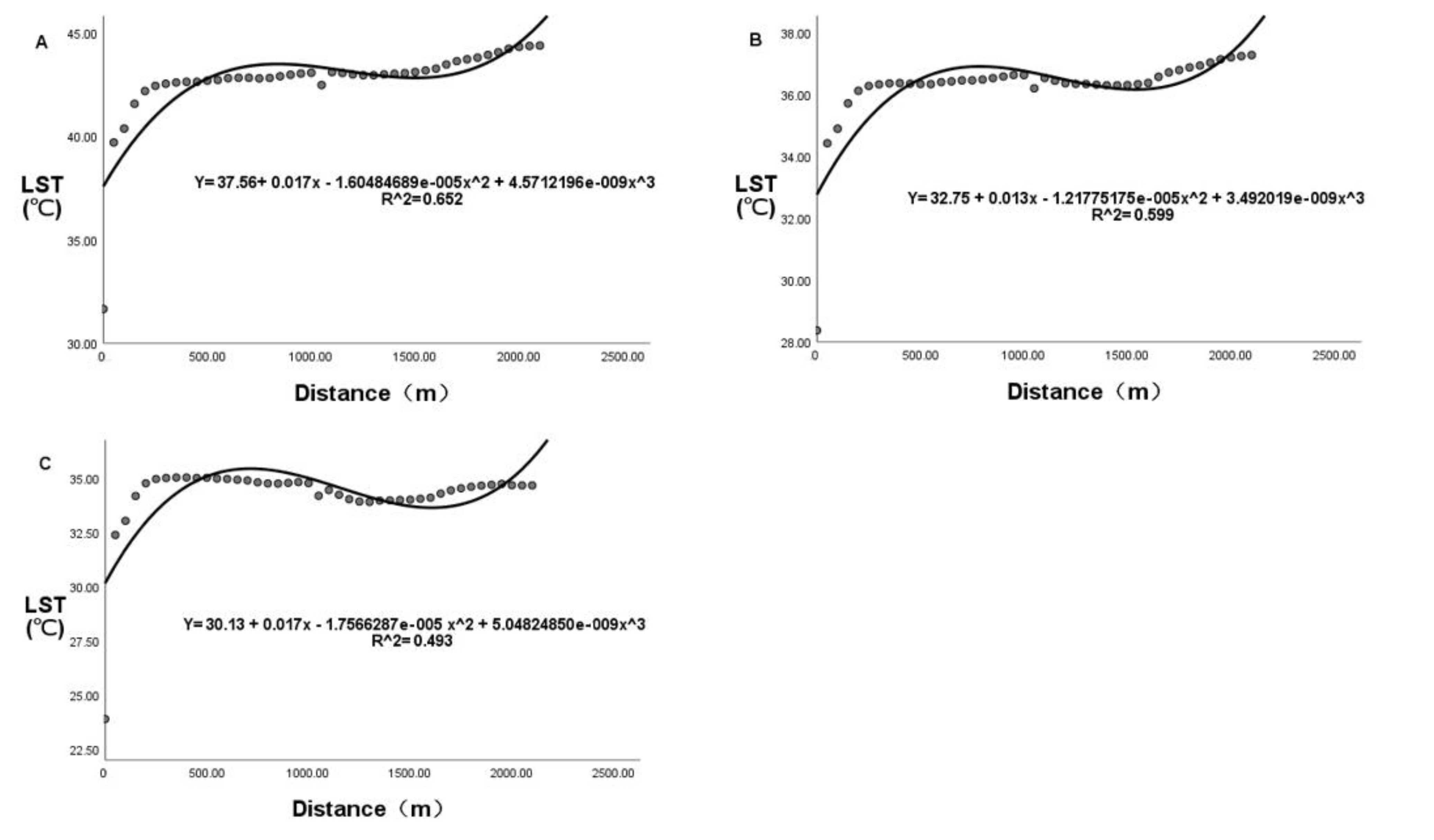
3.3.1. Cooling Intensity and Distance of Water Bodies

From 2010 to 2020, the internal temperature of water bodies and the temperature around water bodies at different distances were analyzed, and the optimal fitting function scheme was explored through curve fitting (Figure 7). Finally, it was concluded that the cubic polynomial fitting scheme was the best, and the mean R2 value of the three-year fitting function was 0.581. The difference between internal temperature and ambient temperature was defined as water bodies cooling effect. The cubic polynomial fitting function showed that the cooling effect of water bodies increased with the distance from water bodies, but only extended to a certain range and then disappeared. WCI and WCD were obtained by calculating the inflection point of the fitting function. In 2020, the WCI and WCD were about 9.70 °C and 861 m, while 7.30 °C and 748 m in 2015, 4.57 °C and 689 m in 2010. The cooling distance of water bodies was about 690 m to 860 m with the average value of 766 m, while the average value of cooling intensity was 6.86 °C.

3.3.2. Cooling Intensity and Distance of Green Spaces

The size of the 311 green samples ranged from 0.09 ha to 39.27 ha, and the LST ranged from 36.92 °C to 47.71 °C (2020). The LST of 354 green samples ranged from 30.47 °C to 42.26 °C (2015) and the LST of 384 green samples ranged from 28.67 °C to 40.04 °C (2010) while the area range identical with 2010. Pearson correlation analysis results indicated that the size of green samples and the LST was significant correlated (r = −0.365, p = 0.01). Due to the obvious difference in area size of green spaces samples, in order to better understand the relationship between green spaces and LST, we classified green samples into larger (10.73–40 ha), medium (3.23–10.72 ha), and small (0.09–3.22 ha) categories based on area size.
Different categories of GCI and GCD were calculated and outliers are removed. Specifically, as Table 4 showed, the average GCI value of all green samples was 1.82 °C (2020), 1.86 °C (2015) and 1.99 °C (2010) respectively. Under the background of increasing urban temperature, the average cooling intensity was roughly the equal for all size groups. The mean GCI of small samples (1.67 °C) was lower than that of medium samples (3.76 °C) in all three years, while medium samples was lower than that of larger samples (3.92 °C). Regarding GCD, ranging from 30 m to 450 m, the average value was 250 m in 2020, 578 m in summer and 238 m in 2010. Larger samples and medium samples had higher GCD than smaller samples in all three years. Meanwhile, the minimum GCD of small samples was 30 m, although medium and larger samples were 120 m. This indicated that with the increase of sample area, the cooling indicator of green spaces would also increase, but the growth rate tended to slow down.

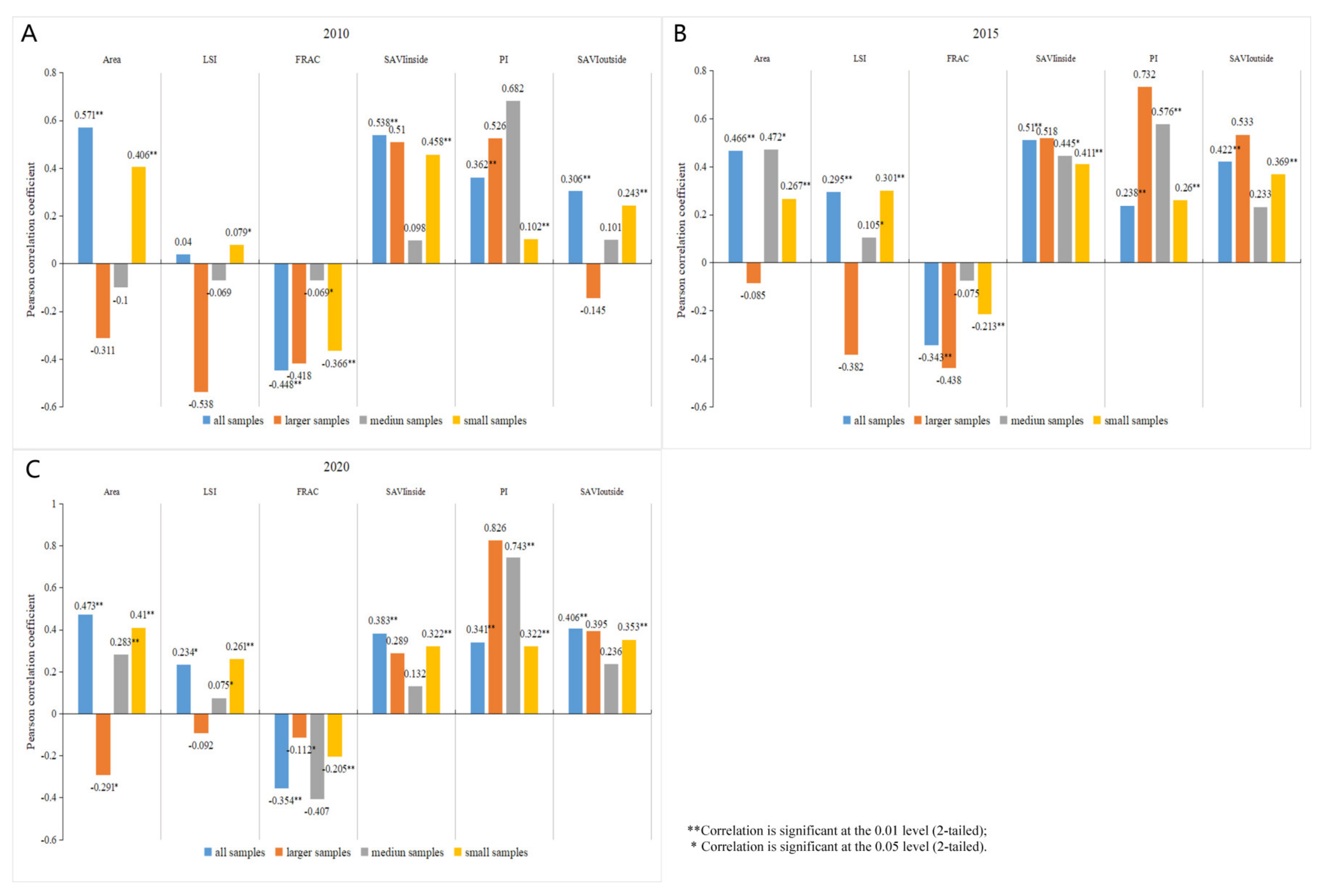
3.4. Relationships between Cooling Indicators and Impacts Factors

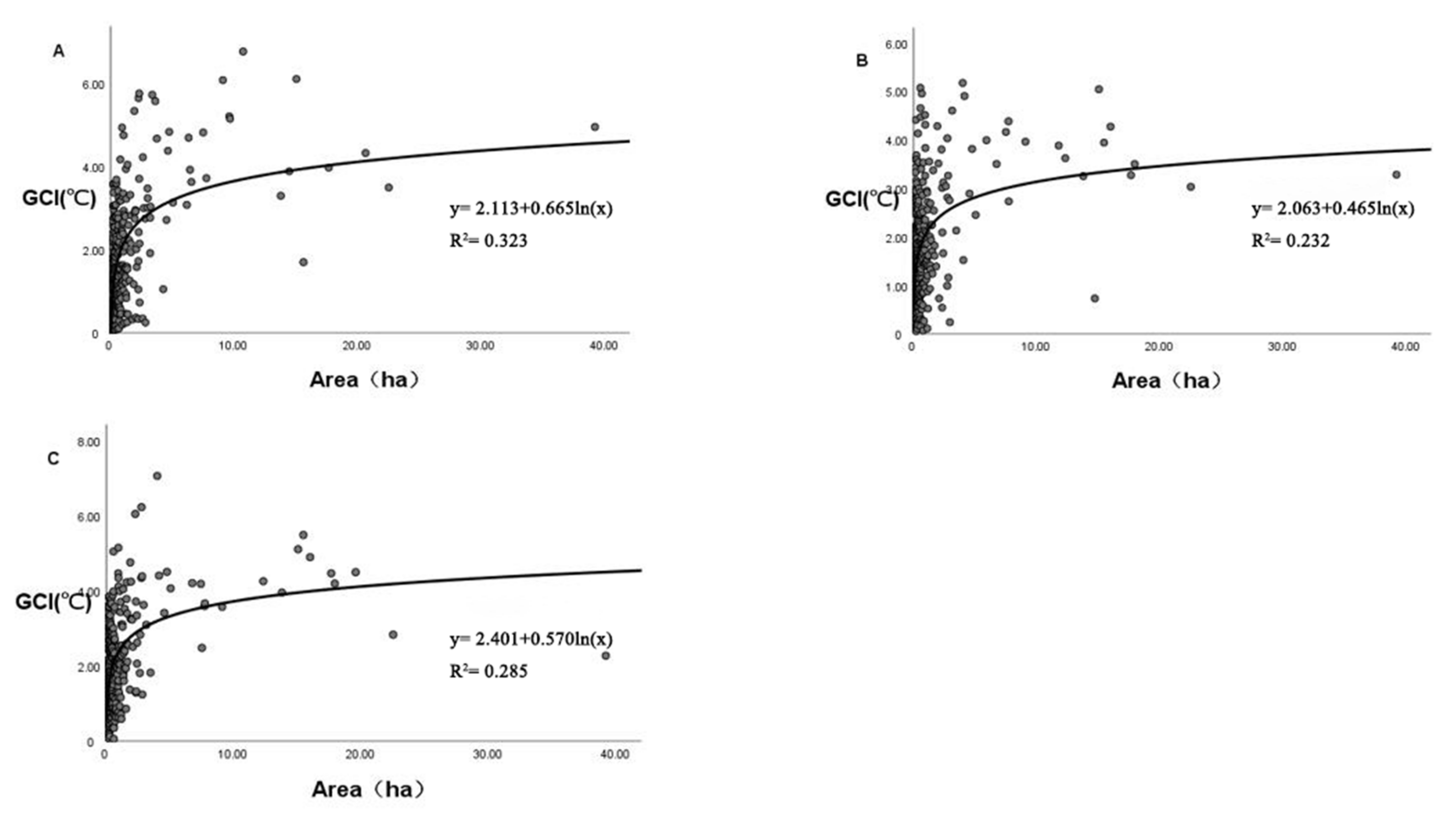
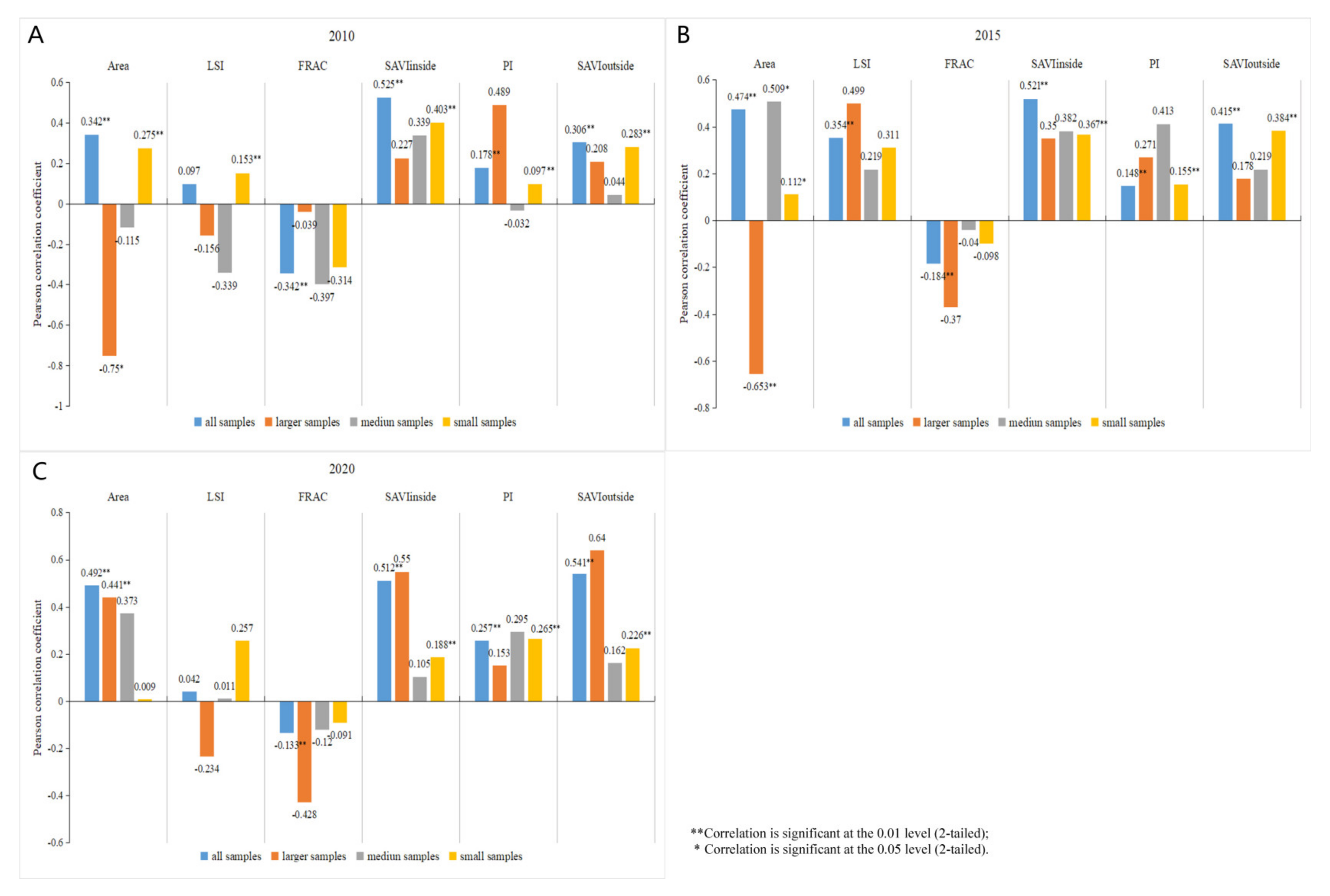
3.4.1. The Impact on Cooling Intensity

The Pearson correlation coefficients between GCI and impact factors were shown in Figure 8. The results showed that internal factors and external factors were significantly correlated with the cooling intensity of green samples. For internal factors, moderately significant positive correlations between area and GCI were found for all samples in 2020 (r = 0.473), 2015 (r = 0.466) and 2010 (r = 0.571), while for medium samples in 2015 (r = 0.472) and for small samples in 2020 (r = 0.41). FRAC had significant negative correlation with GCI in all three years. LSI positively correlated with GCI for all samples in 2020 (r = 0.234) and 2015 (r = 0.295), and a positive relationship was found in 2010 although it was not significant. SAVIinside had moderately significant positive correlations with GCI in all three years (r2020 = 0.383; r2015 = 0.51; r2010 = 0.538). Meanwhile only small samples showed significant correlation, while medium samples and larger samples showed no significant correlation. Among four internal factors (area, LSI, FRAC and SAVIinside), area had the most significant correlation with the cooling intensity, followed by the SAVIinside, then the FRAC, at last the LSI. With regard to external factors, the PI (r2020 = 0.341; r2015 = 0.238; r2010 = 0.362), SAVIoutside (r2020 = 0.406; r2015 = 0.422; r2010 = 0.306) were positively correlated with the cooling intensity. For each year, TVoE was calculated based on the area of green samples were in a logarithmical relationship with the cooling intensity (Figure 9). The TVoE of GCI was 0.67 ha in 2020, 0.47 ha in 2015 and 0.57 ha in 2010. That was to say, the area of green spaces sample was 0.57 ha can effectively and economically alleviate the UHI effect and better benefit the urban population in Fuzhou.

3.4.2. The Impact on Cooling Distance

The Pearson correlation coefficients between GCD and impact factors were illustrated in Figure 10. For internal factors, the area and the SAVIinside showed significantly positive correlations with GCD for all samples in three years. The correlation coefficients varied from 0.342 to 0.525, which indicated moderate relationships between those factors and cooling distance. LSI positively correlated with GCD for all samples in 2015 (r = 0.254). FRAC had significant negative correlation with GCD in all three years, while the relationships exhibit weak correlation (r = −0.220). In details for three green samples size groups, no significant correlation was found between internal factors and GCD. The result could be found which indicated the inconsistency between green samples size groups. Among four internal factors, SAVIinside had the most significant correlation with the cooling distance, followed by the area, then the FRAC. For external factors, the PI and the SAVIoutside were positively correlated with the cooling distance, while SAVIoutside was more correlated than PI.

4. Discussion

4.1. The Difference of Cooling Effect between Water Bodies and Green Spaces

Among water bodies and green spaces, although water bodies has great cooling potential, the investigations on water bodies cooling effect are much less than that of green spaces [22], and the researches on the layout of water bodies and green spaces in the same urban is more rare [27,50]. In this study, hot spot analysis and correlation analysis (LST and coverage) were used to contrast the cooling effect of vegetation and water bodies for the surrounding environment. Quantitative calculation of cooling intensity and cooling distance was applied to characterize the cooling effect of water bodies and green spaces. Then, the correlation analysis (cooling indicators and impacts factors) method was used to explore the influence of internal and external space characteristics of water bodies and green spaces on cooling effect. Further, we tried to explore the TVoE of reference significance for future urban planning.
Both vegetation and water coverage were significantly negatively correlated with LST, indicating that LST would decrease with the continuous increase of vegetation and water coverage. Meanwhile, the correlation between surface temperature and water coverage was more significant than that of vegetation coverage, indicating that the cooling effect of water bodies were stronger than that of green spaces. The conclusion of this study was consistent with most previous studies [51,52,53,54,55]. The possible reasons are differences in urban background conditions, temperature measurement time and season, and conditions inside and outside the sample, such as urban dimension and tree canopy conditions in surrounding cities. A contrary conclusion was drawn in the study of Nanjing [20].
Further, cooling intensity and cooling distance were selected to quantitatively characterize the cooling effect of water bodies and green spaces. Due to the obvious difference in area size of green spaces samples, in order to understand the relationship between green spaces size and LST, we classified green samples into larger, medium, and small categories based on area size. Classification analyses based on the characteristics of green spaces were very common in studying the cooling effect of urban green spaces [16]. From the perspective of cooling intensity, in 2015 and 2020, regardless of the size, the cooling intensity of water bodies (9.70 °C and 7.30 °C, respectively) was greater than that of green spaces (1.86 °C and 1.82 °C, respectively). It is worth noting that this is not the case in all conclusions. In 2010, the cooling intensity of some larger samples of green spaces exceeded that of water bodies in the same year, while the cooling intensity of samples of medium and small areas was less than that of water bodies. The probable reason is that the average background temperature in 2010 was smaller than in other years. When background temperature was high, water bodies may have a stronger cooling potential than green spaces. Both water bodies and green spaces absorbed heat from their surroundings through evapotranspiration, and exchanged cool air into the surrounding hot air through air flow. In addition, the green space can reduce the temperature inside and around the green space by shading and absorbing carbon dioxide. When the background temperature was low, larger area of green spaces would generate larger area of cold islands through shading and absorbing carbon dioxide. However, when the background temperature increased rapidly, the cooling effect generated by the shading and absorbing carbon dioxide of green spaces was not as strong as that generated by the constant temperature water bodies. Besides, the WCD is much larger than the GCD in this study, in accordance with previous studies [52,53,55].
The above conclusions all indicated that in Fuzhou city, where the UHI effect could not be ignored and was becoming increasingly serious, water bodies could bring a stronger cooling effect with longer influence range than green spaces to other surrounding environments, and contribute more energy to alleviate the UHI effect.

4.2. Factors Affecting the Cooling Effect

In order to explore the spatial layout of the optimal green spaces sample, the following internal and external indicators were selected, including area, LSI, and FRAC to represent the sample shape characteristics, and SAVI and PI to represent the different landscape composition of the sample itself and the surrounding environment. Studies showed that the area size of a single sample was significantly positively correlated with GCI and GCD, which was consistent with most studies [46,50,56]. Small samples (area < 3.22 ha) maintained a significant positive correlation in different years, which could be used to support the validity of the conclusion that the efficiency threshold (TVoE) of the average optimal green spaces area was 0.57 ha. However, this phenomenon became blurred with larger samples. Meanwhile, this study concluded that the optimal area of green spaces patch in Fuzhou city with temperate monsoon climate was 0.57 ha, which was similar to the previous research conclusion. Fan’s study showed that TVoE of 7 Low-latitude Asian cities was 0.6–0.95 ha [57]. Yu found that the TVoE of cities in Temperate monsoon and Mediterranean climates was generally around 0.5 ha [30]. Compared with previous studies, the TVoE of green spaces in Fuzhou was 0.57 ha, which was within the error range.
For LSI, the effect of LSI on the cooling effect of green samples remains controversial in previous studies. Part of the conclusion was that LSI of green spaces samples was significantly positively correlated with cooling indicators [58], which was consistent with the conclusion that samples with more complex shapes in 2015 and 2020 could produce stronger cooling intensity. Nevertheless, contrary views were increasing [58,59]. The positive correlation between LSI and cooling indicators was stronger in the small sample than in the large sample. Previous research conclusions in Jaganmohan [60] could support the conclusion of this study. Jaganmohan founded that when the smaller green spaces increased its irregular shape, it would provide a longer interface between the green spaces and surroundings. This provided more opportunities for cooler air to influence the residential surroundings.
Furthermore, SAVIinside and NDVI referred to the greenness of a green spaces sample, which meant the abundance of vegetation biomass. Numerous studies have concluded that NDVI in green spaces had a positive impact on the cooling effect of green spaces [30,31,57]. In this study, both the cooling intensity and cooling distance of green spaces samples were positively correlated with SAVIinside, which indicated that green spaces with higher greenness would provide a stronger cooling effect on a wider range of surrounding environment, especially the small green spaces.
Besides, in previous studies on water bodies cooling effect and urban park cooling effect [22,35,55,61], external factors of samples were often selected to study the degree of influence on the cooling indicators, while the methods were rarely put into use in the study of green spaces, so this study selected the external factors of green spaces to discuss the degree of influence on the indicators. The higher the PI around small samples, the stronger the cooling intensity of the samples from 2010–2020, which meant that in the region with higher building coverage, adding a small sample of green spaces was more effective in alleviating the UHI effect of the surrounding environment. SAVIoutside had moderately significant positive correlations with GCI in all three years, illustrating that green spaces had stronger cooling intensity in region with higher overall greening rate.

4.3. Implications for Urban Planning and Management

The effect mechanism of vegetation coverage and water coverage on LST in different streets was studied, and the cooling index of different samples in the water bodies and green spaces was quantitatively analyzed and obtained. In addition, the internal shape, biological characteristics, and external landscape composition of samples were selected as influencing factors to explore the relationship between the cooling indicators and the sample. The qualitative and quantitative results provided important suggestions and inspirations for the macro-management regulation and micro-layout planning of urban water bodies and green spaces respectively.
Vegetation coverage and water coverage were negatively correlated with LST, and water coverage had a stronger effect on LST. On this basis, based on street data, it was found that the relationship between water bodies, vegetation coverage and LST was logarithmic, which meant that increasing water bodies and vegetation coverage in streets where people live could effectively reduce LST and alleviate the UHI effect. However, such a logarithmic relationship meant that the LST decreased with the increase of coverage, and the rate of decline continued to slow down. Especially when the slope of a logarithmic function was equal to 1, the decreasing efficiency of LST would become very slow. At the same time, the proportion of impervious surfaces in the streets in the urban core region was very high, so it was difficult to provide sufficient public service areas to layout more water bodies and vegetation. Therefore, it is meaningful to study the optimal value of vegetation coverage and water coverage in each street [62,63,64]. Combined with the actual situation, under the background of urban development, it was suggested to increase the reasonable layout of water bodies. In addition, the recommended range of vegetation coverage is 0–27%, which provided macroscopical thinking inspiration for future urban planning and layout.
The area is an important factor affecting the cooling effect of a single green sample. In-depth investigation showed that with the increase of sample area, the maximum temperature difference between the sample and the surrounding environment also increased, but this relationship was not linear [27]. From 2010 to 2020, the average cooling intensity difference between larger samples and medium samples was much smaller than the average cooling intensity difference between medium samples and small samples, as well as the cooling range. Combined with regression analysis, the average TVoE was 0.57 ha, indicating that the area of green spaces without cooling synergistic effect was the most economical and effective to reduce the ambient temperature at 0.57 ha.
According to the conclusion in 4.3, in the future planning and layout of small samples of green spaces, we found that the shape characteristics (LSI) and biological characteristics (SAVIinside) of green spaces were important factors affecting the cooling effect. However, in the core region of Fuzhou, the green spaces are usually the green belt along the road or the park with a larger area, which can be planned as larger green spaces with a higher degree of greenness and provide more ecosystem services. The critical value of urban green spaces and the influence of it features on the cooling effect still remain to be investigated. In this paper, TVoE idea was used to propose that 0.57 ha green spaces with high irregularity and greenness was the best green spaces condition for effectively alleviating UHI effect, which had certain reference significance for urban planners and decision makers.

4.4. Limitations of the Study

Some limitations of this study are the direction of future research. First of all, remote sensing image data of one day in summer of different years were used in this study to present temporal variation, ignoring seasonal and diurnal variation, which would lead to certain one-sidedness and uncertainty in the research results. It is an important direction to use different methods to obtain temperature data and to explore the influence of time difference on the cooling effect from a more comprehensive perspective. Secondly, many studies in which the cooling effect of green spaces has been examined using computer simulation based on several scenarios regarding the specifications of the green spaces [16]. The future research direction of this study is to separately analyze the cooling effect of each green spaces on a smaller scale. Furthermore, with the gradual fragmentation of water bodies and green spaces in the metropolis, especially in densely built-up areas [65,66], the interaction between the water bodies and green spaces becomes hard to ignore. Special attention should pay to future research. In addition, the optimal area (TVoE) was quantitatively calculated in this study, but the meaning of TVoE for future urban planning is still vague [27]. Future studies of this topic should be devoted to in-depth exploration of the mechanism and influencing factors of TVoE, so as to find out the optimal spatial pattern.

5. Conclusions

This study focused on urban water bodies and green spaces planning to alleviate the phenomenon of rising summer temperature in the Fuzhou city. In this study, we compared the cooling effect of water bodies and green spaces on the surrounding environment from different standpoints, quantified the cooling intensity and cooling distance of samples, and explored the correlation between cooling indicators and the internal and external spatial characteristics of samples. The following conclusions were drawn: (1) The cooling effect of water bodies were stronger than that of vegetation in most cases, especially under the background of rising urban temperature; (2) More water bodies’ layout in the region was advocated. Considering the actual situation, increasing vegetation coverage within 27% of the region can effectively and economically alleviate the thermal environment in areas with a large number of human production activities; (3) From 2010 to 2020, the GCI was about 0.06 °C to 6.10 °C with an average value of 1.89 °C while the GCD was about 30 m to 450 m with an average value of 240 m; (4) The WCI is about 4.57 °C to 9.70 °C with an average value of 6.86 °C while the WCD was about 690 m to 860 m with an average value of 766 m; (5) The average value of TVoE was 0.57 ha. In the planning of green spaces, the optimal area was 0.57 ha, and irregular green spaces samples with high vegetation index had high cost performance to alleviate the phenomenon of high temperature in the surrounding environment. The results provide quantitative guidance for urban public service spatial planning of water bodies and green spaces to prevent the continuous increase of urban background temperature.

Author Contributions

Y.-B.C. designed the overall ideas and drawn up the research goals. Y.-B.C. and Z.-J.W. performed data process and analysis. Y.-H.C., Z.-J.W. and L.W. wrote this initial article and all authors participated in the optimization of the article. W.-B.P. was responsible for the quality and academic value of the articles. All authors have read and agreed to the published version of the manuscript.

Funding

Education Scientific Research Project of Fujian Province Education Department (No. JAT200936). Undergraduate Raining Program for Innovation and Entrepreneurship Project of Fujian Province (No. S202113470016). The national demonstration area of ecological civilization construction innovative technical services in Gulou District of Fuzhou City (No. 00602102).

Institutional Review Board Statement

Not applicable.

Informed Consent Statement

Not applicable.

Data Availability Statement

Not applicable.

Acknowledgments

We are sincerely grateful to U.S. Geological Survey for Landsat image and data processing, to Chinese Academy of Sciences for reference data. We greatly appreciate numerous volunteers for field survey. Furthermore, we feel indebted to three anonymous reviewers for their valuable comments and suggestions on adequately advancing the quality of this manuscript.

Conflicts of Interest

The authors declare no conflict of interest.

References

  1. United Nations Environment Programme. Special Report: Emissions Gap Report 2021: The Heat Is On. Available online: https://www.un.org/zh/156951 (accessed on 26 October 2021).
  2. Oke, T.R. The energetic basis of the urban heat island. Q. J. R. Meteorol. Soc. 1982, 108, 1–24. [Google Scholar] [CrossRef]
  3. Sun, R.; Wang, Y.; Chen, L.A. Distributed model for quantifying temporal-spatial patterns of anthropogenic heat based on energy consumption. J. Clean. Prod. 2018, 170, 601–609. [Google Scholar] [CrossRef]
  4. Ward, K.; Lauf, S.; Kleinschmit, B.; Endlicher, W. Heat waves and urban heat islands in Europe: A review of relevant drivers. Sci. Total Environ. 2016, 569/570, 527–539. [Google Scholar] [CrossRef] [PubMed]
  5. Cai, Y.B.; Zhang, H.; Zheng, P.; Pan, W.B. Quantifying the Impact of Land use/Land Cover Changes on the Urban Heat Island: A Case Study of the Natural Wetlands Distribution Area of Fuzhou City, China. Wetlands 2016, 36, 285–298. [Google Scholar] [CrossRef]
  6. Guo, G.H.; Wu, Z.F.; Xiao, R.B.; Chen, Y.B.; Liu, X.N.; Zhang, X.S. Impacts of urban biophysical composition on land surface temperature in urban heat island clusters. Landsc. Urban Plan. 2015, 135, 1–10. [Google Scholar] [CrossRef]
  7. Li, J.; Song, C.; Cao, L.; Zhu, F.; Wu, J. Impacts of landscape structure on surface urban heat islands: A case study of Shanghai, China. Remote Sens. Environ. 2011, 115, 3249–3263. [Google Scholar] [CrossRef]
  8. Sarrat, C.; Lemonsu, A.; Masson, V.; Guedalia, D. Impact of urban heat island on regional atmospheric pollution. Atmos. Environ. 2006, 40, 1743–1758. [Google Scholar] [CrossRef]
  9. Santamouris, M.; Cartalis, C.; Synnefa, A.; Kolokotsa, D. On the impact of urban heat island and global warming on the power demand and electricity consumption of buildings-A review. Energy Build. 2015, 98, 119–124. [Google Scholar] [CrossRef]
  10. Wang, Y.; Wang, A.; Zhai, J.; Tao, H.; Jiang, T.; Su, B.; Yang, J.; Wang, G.; Liu, Q.; Gao, C. Tens of thousands additional deaths annually in cities of China between 1.5 °C and 2.0 °C warming. Nat. Commun. 2019, 10, 3376. [Google Scholar] [CrossRef]
  11. Taylor, J.; Wilkinson, P.; Davies, M.; Armstrong, B.; Chalabi, Z.; Mavrogianni, A.; Symonds, P.; Oikonomou, E.; Bohnenstengel, S.I. Mapping the effects of urban heat island, housing, and age on excess heat-related mortality in London. Urban Clim. 2015, 14, 517–528. [Google Scholar] [CrossRef]
  12. Seto, K.C.; Golden, J.S.; Alberti, M.; Turner, B.L. Sustainability in an urbanizing planet. Proc. Natl. Acad. Sci. USA 2017, 114, 8935–8938. [Google Scholar] [CrossRef] [PubMed] [Green Version]
  13. Mora, C.; Dousset, B.; Caldwell, I.R.; Powell, F.E.; Geronimo, R.C.; Bielecki, C.R.; Counsell, C.; Dietrich, B.S.; Johnston, E.T.; Louis, L.V. Global risk of deadly heat. Nat. Clim. Change 2017, 7, 501–506. [Google Scholar] [CrossRef]
  14. Akbari, H.; Kolokotsa, D. Three decades of urban heat islands and mitigation technologies research. Energy Build 2016, 133, 834–842. [Google Scholar] [CrossRef]
  15. Solcerova, A.; van de Ven, F.; Wang, M.; Rijsdijk, M.; van de Giesen, N. Do green roofs cool the air? Build. Environ. 2017, 111, 249–255. [Google Scholar] [CrossRef] [Green Version]
  16. Aram, F.; Higueras, G.E.; Solgi, E.; Mansournia, S. Urban green space cooling effect in cities. Heliyon 2019, 5, e01339. [Google Scholar] [CrossRef] [PubMed] [Green Version]
  17. Zheng, H.Z.; Chen, Y.H.; Pan, W.B.; Cai, Y.B.; Chen, Z.J. Impact of Land Use/Land Cover Changes on the Thermal Environment in Urbanization: A Case Study of the Natural Wetlands Distribution Area in Minjiang River Estuary, China. Pol. J. Environ. Stud. 2019, 28, 3025–3041. [Google Scholar] [CrossRef]
  18. Kolokotroni, M.; Giannitsaris, I.; Watkins, R. The effect of the London urban heat island on building summer cooling demand and night ventilation strategies. Sol. Energy 2006, 80, 383–392. [Google Scholar] [CrossRef]
  19. Lin, M.X.; Dong, J.; Jones, L.; Liu, J.k.; Lin, T.; Zuo, J.; Ye, H.; Zhang, G.Q.; Zhou, T.J. Modeling green roofs’cooling effect in high-density urban areas based on law of diminishing marginal utility of the cooling efficiency: A case study of Xiamen Island, China. J. Clean. Prod. 2021, 316, 128277. [Google Scholar] [CrossRef]
  20. Feyisa, G.L.; Dons, K.; Meilby, H. Efficiency of parks in mitigating urban heat island effect: An example from Addis Ababa. Landsc. Urban Plan. 2014, 123, 87–95. [Google Scholar] [CrossRef]
  21. Sun, X.; Tan, X.; Chen, K.; Song, S.; Hou, D. Quantifying landscape-metrics impacts on urban green-spaces and water-bodies cooling effect: The study of Nanjing, China. Urban For. Urban Green. 2020, 55, 126838. [Google Scholar] [CrossRef]
  22. Wang, Y.; Ouyang, W. Investigating the heterogeneity of water cooling effect for cooler cities. Sustain. Cities Soc. 2021, 75, 103281. [Google Scholar] [CrossRef]
  23. Rahman, M.A.; Moser, A.; Rötzer, T.; Pauleit, S. Within canopy temperature differences and cooling ability of Tilia cordata trees grown in urban conditions. Build. Environ. 2017, 114, 118–128. [Google Scholar] [CrossRef]
  24. Doick, K.J.; Peace, A.; Hutchings, T.R. The role of one large greenspace in mitigating London’s nocturnal urban heat island. Sci. Total Environ. 2014, 493, 662–671. [Google Scholar] [CrossRef] [PubMed]
  25. Volker, S.; Baumeister, H.; Classen, T.; Hornberg, C.; Kistemann, T. Evidence for the temperature-mitigating capacity of urban blue space-a health geographic perspective. Erdkunde 2013, 67, 355–371. [Google Scholar] [CrossRef]
  26. Martins, T.A.L.; Adolphe, L.; Bonhomme, M.; Bonneaud, F.; Guyard, W. Impact of Urban Cool Island measures on outdoor climate and pedestrian comfort: Simulations for a new district of Toulouse, France. Sustain. Cities Soc. 2016, 26, 9–26. [Google Scholar] [CrossRef]
  27. Yu, Z.; Yang, G.; Zuo, S.; Jrgensen, G.; Vejre, H. Critical review on the cooling effect of urban blue-green space: A threshold-size perspective. Urban For. Urban Green. 2020, 49, 126630. [Google Scholar] [CrossRef]
  28. Santamouris, M.; Ban-Weiss, G.; Osmond, P.; Paolini, R. Progress in urban greenery mitigation science-assessment methodologies advanced technologies and impact on cities. J. Civ. Eng. Manag. 2018, 24, 638–671. [Google Scholar] [CrossRef] [Green Version]
  29. Yu, Z.; Yao, Y.; Yang, G.; Wang, X.; Vejre, H. Strong contribution of rapid urbanization and urban agglomeration development to regional thermal environment dynamics and evolution. For. Ecol. Manag. 2019, 446, 214–225. [Google Scholar] [CrossRef]
  30. Peng, J.; Dan, Y.; Qiao, R.; Liu, Y.; Wu, J. How to quantify the cooling effect of urban parks? Linking maximum and accumulation perspectives. Remote Sens. Environ. 2021, 252, 112135. [Google Scholar] [CrossRef]
  31. Kuang, W.; Liu, Y.; Dou, Y.; Chi, W.; Chen, G.; Gao, C.; Yang, T.; Liu, J.; Zhang, R. What are hot and what are not in an urban landscape: Quantifying and explaining the land surface temperature pattern in Beijing, China. Landsc. Ecol. 2015, 30, 357–373. [Google Scholar] [CrossRef]
  32. Yu, Z.; Guo, X.; Jørgensen, G.; Vejre, H. How can urban green spaces be planned for climate adaptation in subtropical cities? Ecol. Indic. 2017, 82, 152–162. [Google Scholar] [CrossRef]
  33. Derkzen, M.L.; Van, T.A.; Verburg, P.H. Green infrastructure for urban climate adaptation: How do residents’ views on climate impacts and green infrastructure shape adaptation preferences? Landsc. Urban Plan. 2017, 157, 106–130. [Google Scholar] [CrossRef]
  34. Du, H.; Song, X.; Jiang, H.; Kan, Z.; Wang, Z.; Cai, Y. Research on the cooling island effects of water body: A case study of Shanghai, China. Ecol. Indic. 2016, 67, 31–38. [Google Scholar] [CrossRef]
  35. Peng, J.; Liu, Q.; Xu, Z.; Lyu, D.; Wu, J. How to effectively mitigate urban heat island effect? A perspective of waterbody patch size threshold. Landsc. Urban Plan. 2020, 202, 103873. [Google Scholar] [CrossRef]
  36. Liao, W.; Cai, Z.W.; Feng, Y.; Gan, D.X.; Li, X.M. A simple and easy method to quantify the cool island intensity of urban greenspace. Urban For. Urban Green. 2021, 62, 127173. [Google Scholar] [CrossRef]
  37. Yu, K.; Chen, Y.; Liang, L.; Gong, A.; Li, J. Quantitative analysis of the interannual variation in the seasonal water cooling island (WCI) effect for urban areas. Sci. Total Environ. 2020, 727, 138750. [Google Scholar] [CrossRef] [PubMed]
  38. Cai, Y.B.; Li, H.M.; Ye, X.Y.; Zhang, H. Analyzing Three-Decadal Patterns of Land Use/Land Cover Change and Regional Ecosystem Services at the Landscape Level: Case Study of Two Coastal Metropolitan Regions, Eastern China. Sustainability 2016, 8, 773. [Google Scholar] [CrossRef] [Green Version]
  39. Cai, Y.B.; Zhang, H.; Pan, W.B. Detecting Urban Growth Patterns and Wetland Conversion Processes in a Natural Wetlands Distribution Area. Pol. J. Environ. Stud. 2015, 24, 1919–1929. [Google Scholar] [CrossRef]
  40. Cai, Y.B.; Zhang, H.; Pan, W.B.; Chen, Y.H.; Wang, X.R. Urban expansion and its influencing factors in Natural Wetland Distribution Area in Fuzhou City, China. Chin. Geogr. Sci. 2012, 22, 568–577. [Google Scholar] [CrossRef]
  41. Li, K.; Cai, Y.B.; Chen, Y.H.; Wu, L.; Pan, W.B. The Changes of Heat Contribution Index in Urban Thermal Environment: A Case Study in Fuzhou. Sustainability 2021, 13, 9638. [Google Scholar]
  42. Cai, Y.B.; Chen, Y.; Tong, C. Spatiotemporal evolution of urban green space and its impact on the urban thermal environment based on remote sensing data: A case study of Fuzhou City, China. Urban For. Urban Green. 2019, 41, 333–343. [Google Scholar] [CrossRef]
  43. Cai, Y.B.; Zhang, H.; Pan, W.B.; Chen, Y.H.; Wang, X.R. Land use pattern, socio-economic development, and assessment of their impacts on ecosystem service value: Study on natural wetlands distribution area (NWDA) in Fuzhou city, southeastern China. Environ. Monit. Assess. 2013, 185, 5111–5123. [Google Scholar] [CrossRef] [PubMed]
  44. Yu, X.; Guo, X.; Wu, Z. Land Surface Temperature Retrieval from Landsat 8 TIRS—Comparison between Radiative Transfer Equation-Based Method, Split Window Algorithm and Single Channel Method. Remote Sens. 2014, 6, 9829–9852. [Google Scholar] [CrossRef] [Green Version]
  45. Xu, H.Q. Remote sensing information extraction of urban building land based on compressed data dimension. J. Image Graph. 2005, 10, 223–229. [Google Scholar]
  46. Monteiro, M.V.; Doick, K.J.; Handley, P.; Peace, A. The impact of greenspace size on the extent of local nocturnal air temperature cooling in London. Urban For. Urban Green. 2016, 16, 160–169. [Google Scholar] [CrossRef]
  47. Xu, H.Q. study on information extraction of water body with the modified normalized difference water index (MNDWI). J. Remote Sens. 2005, 9, 595. (In Chinese) [Google Scholar]
  48. Qiu, K.; Jia, B. The roles of landscape both inside the park and the surroundings in park cooling effect. Sustain. Cities Soc. 2020, 52, 101864. [Google Scholar] [CrossRef]
  49. Sun, R.; Chen, L. How can urban water bodies be designed for climate adaptation? Landsc. Urban Plan. 2012, 105, 27–33. [Google Scholar] [CrossRef]
  50. Yang, G.; Yu, Z.; Jørgensen, G.; Vejre, H. How can urban blue-green space be planned for climate adaption in high-latitude cities? A seasonal perspective. Sustain. Cities Soc. 2020, 53, 101932. [Google Scholar] [CrossRef]
  51. Yu, Z.W.; Guo, X.Y.; Zeng, Y.X.; Koga, M.; Vejre, H. Variations in land surface temperature and cooling efficiency of green space in rapid urbanization: The case of Fuzhou city, China. Urban For. Urban Green. 2018, 29, 113–121. [Google Scholar] [CrossRef]
  52. Lee, D.; Oh, K.; Seo, J. An Analysis of Urban Cooling Island (UCI) Effects by Water Spaces Applying UCI Indices. International J. Environ. Sci. Dev. 2016, 7, 810–815. [Google Scholar] [CrossRef] [Green Version]
  53. Lin, W.; Yu, T.; Chang, X.; Wei, W.; Yue, Z. Calculating cooling extents of green parks using remote sensing: Method and test. Landsc. Urban Plan. 2015, 134, 66–75. [Google Scholar] [CrossRef]
  54. Gunawardena, K.R.; Wells, M.J.; Kershaw, T. Utilising green and blue space to mitigate urban heat island intensity. Sci. Total Environ. 2017, 584-585, 1040–1055. [Google Scholar] [CrossRef] [PubMed]
  55. Cai, Z.; Han, G.; Chen, M. Do water bodies play an important role in the relationship between urban form and land surface temperature? Sustain. Cities Soc. 2018, 39, 487–498. [Google Scholar] [CrossRef]
  56. Bowler, D.E.; Buyung-Ali, L.; Knight, T.M.; Andrew, S.P. Urban greening to cool towns and cities: A systematic review of the empirical evidence. Landsc. Urban Plan. 2010, 97, 147–155. [Google Scholar] [CrossRef]
  57. Fan, H.; Yu, Z.; Yang, G.; Liu, T.Y.; Hung, C.H.; Vejre, H. How to cool hot-humid (Asian) cities with urban trees? An optimal landscape size perspective. Agric. For. Meteorol. 2019, 265, 338–348. [Google Scholar] [CrossRef]
  58. Ke, X.; Men, H.; Zhou, T.; Li, Z.Y.; Zhu, F.K. Variance of the impact of urban green space on the urban heat island effect among different urban functional zones: A case study in Wuhan. Urban For. Urban Green. 2021, 62, 127159. [Google Scholar] [CrossRef]
  59. Kong, F.; Yin, H.; James, P.; Hutyra, L.R.; He, H.S. Effects of spatial pattern of greenspace on urban cooling in a large metropolitan area of eastern China. Landsc. Urban Plan. 2014, 128, 35–47. [Google Scholar] [CrossRef]
  60. Jaganmohan, M.; Knapp, S.; Buchmann, C.M.; Schwarz, N. The bigger, the better? The influence of urban green space design on cooling effects for residential areas. J. Environ. Qual. 2016, 45, 134–145. [Google Scholar] [CrossRef]
  61. Zheng, Y.; Li, Y.; Hou, H.; Murayama, Y.; Hu, T. Quantifying the Cooling Effect and Scale of Large Inner-City Lakes Based on Landscape Patterns: A Case Study of Hangzhou and Nanjing. Remote Sens. 2021, 13, 1526. [Google Scholar] [CrossRef]
  62. Peng, J.; Xie, P.; Liu, Y.; Jing, M. Urban thermal environment dynamics and associated landscape pattern factors: A case study in the Beijing metropolitan region. Remote Sens. Environ. 2016, 173, 145–155. [Google Scholar] [CrossRef]
  63. Shih, W. Greenspace patterns and the mitigation of land surface temperature in Taipei metropolis. Habitat Int. 2017, 60, 69–80. [Google Scholar] [CrossRef]
  64. Ren, Z.; He, X.; Pu, R.; Zheng, H. The impact of urban forest structure and its spatial location on urban cool island intensity. Urban Ecosyst. 2018, 21, 863–874. [Google Scholar] [CrossRef]
  65. Li, F.Z.; Zheng, W.; Wang, Y.; Liang, J.H.; Xie, S.; Guo, S.Y.; Li, X.; Yu, C.M. Urban Green Space Fragmentation and Urbanization: A Spatiotemporal Perspective. Forests 2019, 10, 333. [Google Scholar] [CrossRef] [Green Version]
  66. Lin, Y.; An, W.; Gan, M.; Shahtahmassebi, A.; Huang, L.Y.; Zhu, W.; Huang, L.; Zhang, J.; Wang, K. Spatial Grain Effects of Urban Green Space Cover Maps on Assessing Habitat Fragmentation and Connectivity. Land 2021, 10, 1065. [Google Scholar] [CrossRef]
Figure 1. Location of the core urban area of Fuzhou.
Water 14 01471 g001
Figure 2. Distribution of LST.
Water 14 01471 g002
Figure 3. Spatial distribution of water bodies and green spaces.
Water 14 01471 g003
Figure 4. Figure out the calculation of cooling indicators.
Water 14 01471 g004
Figure 5. Spatial pattern of LST in 2015 (A,B) cold-hot spot areas, Yushan Scenic Area (C) and Changanshan Scenic Area (E), spatial distribution of LST in Yushan Scenic Area in 2015 (D) and analysis of cold hot spots in Changanshan Scenic Area in 2015 (F).
Water 14 01471 g005
Figure 6. Relationship between LST and water coverage as well as vegetation coverage in (A,D) 2020, (B,E) 2015 and (C,F) 2010.
Water 14 01471 g006
Figure 7. Scatter plots of the LST and distances to the water bodies patch in (A) 2010, (B) 2015 and (C) 2020.
Water 14 01471 g007
Figure 8. Pearson correlation coefficients between GCI and impact factors in (A) 2010, (B) 2015 and (C) 2020.
Water 14 01471 g008
Figure 9. Logarithmical relationship between GCI and the green samples in (A) 2020, (B) 2015 and (C) 2010.
Water 14 01471 g009
Figure 10. Pearson correlation coefficients between GCD and impact factors in (A) 2010, (B) 2015 and (C) 2020.
Water 14 01471 g010
Table 1. Descriptions of internal and external factors.
ClassificationAbbreviationDescription
Internal factorsArea (ha)Patch area of the samples
LSILSI (Landscape Shape Index) is a standardized measure of total edge or edge density that
adjusts for the size of the landscape
FRACFRAC (fractal dimension index) is the fractal
dimension of a sample patch
SAVIinsideThe average value of (The Soil Adjusted
Vegetation Index) within the sample
External factorsPI (%)The proportion of impervious surface in the range of cooling effect generated by the sample
SAVIoutsideThe average value of SAVI in the range of
cooling effect generated by the sample
Table 2. LST from 2010–2020.
Date2010.05.242015.09.272020.07.22
Max49.30 °C51.00 °C53.00 °C
Min21.32 °C20.51 °C20.30 °C
Mean32.65 °C34.82 °C40.92 °C
Table 3. Pearson correlation coefficients for LST associated with vegetation and water coverage.
Water CoverageVegetation Coverage
2020−0.708 **−0.360 *
2015−0.722 **−0.366 *
2010−0.721 **−0.519 **
** Correlation is significant at the 0.01 level (2-tailed); *: Correlation is significant at the 0.05 level (2-tailed).
Table 4. Descriptive Statistics of GCI and GCD.
201020152020
MaxMinMeanStdMaxMinMeanStdMaxMinMeanStd
GCI (°C)all samples5.480.061.991.235.040.061.861.116.100.031.821.34
larger samples5.482.284.180.985.042.733.641.016.101.704.961.20
medium samples4.061.823.941.674.171.163.111.285.761.054.231.33
small samples3.220.061.851.123.950.061.550.984.050.031.621.14
GCD (m)all samples45030250.17113.9245030238.05140.2745030248.30136.92
larger samples450150340.00114.02450150351.8291.43450120318.75111.18
medium samples450240327.6966.01450120340.91115.32450120296.25111.17
small samples45030244.70132.4745030228.03138.7845030243.65137.81
Publisher’s Note: MDPI stays neutral with regard to jurisdictional claims in published maps and institutional affiliations.

