Modeling Average Grain Velocity for Rectangular Channel Using Soft Computing Techniques

Abstract

This study was undertaken with the primary objective of modeling grain velocity based on experimental data obtained under the controlled conditions of a laboratory using a rectangular hydraulic tilting channel. Soft computing approaches, i.e., support vector machine (SVM), artificial neural network (ANN), and multiple linear regression (MLR), were applied to simulate grain velocity using four input variables; shear velocity, exposed area to base area ratio (EATBAR), relative depth, and sediment particle weight. Quantitative performance evaluation of predicted values was performed with the help of three different standard statistical indices, such as the root mean square error (RMSE), Pearson’s correlation coefficient (PCC), and Wilmot index (WI). The results during the testing phase revealed that the SVM model has RMSE (m/s), PCC, and WI values obtained as 0.1195, 0.8877, and 0.7243, respectively, providing more accurate predictions than the MLR and ANN models during the testing phase.

1. Introduction

In rivers, sediment grain velocity measurement is generally required to assess sediment load, river geometry, flood control, and long-term morphology evolution. A large number of variables govern the sediment movement process. Thus, its physical measurements under actual field conditions become difficult. Alternatively, experiments are conducted under controlled laboratory conditions to observe the sediment particle movement phenomenon and record data to develop mathematical models for sediment grain velocity. Consequently, experiments were conducted in this study considering a single grain moving near the channel bed due to sliding. These experiments indicated that sediment transport is an incredibly complicated mechanism. It may not be possible to describe it using simple deterministic models. The predictive precision is always doubtful, with predictive errors in several realistic cases being unacceptably high, as is investigated and reported [1,2,3,4]. Therefore, to model sediment grain velocity, the application of new modeling approaches such as machine learning (ML) soft computing techniques have arisen to establish models that rely on experience and data [5,6]. This has opened up new modeling possibilities, mainly when the information available is insufficient to devise a relevant mathematical structure, or there is too little data to calibrate an acceptable model.

Novak and Nalluri [7] examined the incipient motion in fixed, flat, rough beds with roughness elements smaller than the particle size for single and clustered particles. Van Rijn [2] and Karimaee Tabarestani and Zarrati [8] have carried out such regression experiments ostensibly involving the fluid viscous effects on the bedload grain flow in the bed. Papanicolaou et al. [9] estimated the bedload using the idea of particle velocity. Julien and Bounvilay [10] investigated the effect of particles of different sizes with different densities on reach-average bedload particle velocity for smooth and rough surfaces. The impact of the roughness of the bed on the bedload sediment grain velocity was reported by Cheng and Emadzadeh [11]. Frey [12] worked on the fluid velocity of particles and examined the concentration-depth profiles for bedload transport on a high slope at the particle scale. All this research focused on the effects on sediment motion considering the characteristics of channel bed and sediment particles properties.

Further, machine learning (ML) is often considered a replacement or augmentation to the more conventional physical process simulation approach in nearly all research branches. ML uses modeling approaches and techniques such as ANN, SVM, fuzzy logic, decision-tree processes, and improved computing techniques [13,14,15,16,17]. In recent times, several research departments have been influenced by the artificial neural networks (ANN) approach. The ANN method is quickly gaining traction as a useful tool for delivering effective details on the usage in design and management operations for hydraulic, hydrological, and environment fields [18,19,20,21,22]. ML has been efficient for application in the hydrological processes field, e.g., water system management, water quality evaluations, stage-discharge relations, and meteorological data estimations. These implementations, however, demonstrate that ML does not produce new process information. Instead, it uses existing process knowledge to pick the input and output variables, accompanied by sophisticated regression techniques, to the best match for the calculated results. Bhattacharya et al. [23] evaluated sediment transport modeling using ML models such as ANN and model trees. These models used calculated data to model the bedload estimate and total load transport. ANN and regression models to estimate the incipient flow velocity at sediment deposition in the rectangular channel were developed by Sheikh Khozani et al. [24]. Combining the available data from each cross-section created a generalized regression model. Based on the performance assessment, they found ANN models superior to regression models. Mehr and Safari [25] applied soft computing techniques to obtain correct sewer designs via particle Froude number estimates in sewer pipes, including multi genetic programming, gene expression, and multilayer perceptron. Montes et al. [26] have predicted bedload sediment transportation in sewage pipes of noncoherent material using polynomial regression, which describes multiple objective genetic algorithms. In forecasting incipient sediment movement in sewers using artificial neural networks, Wan Mohtar et al. [27] found the impact of bed deposits. Thus, many researchers have shown that the ML approach establishes relationships and is applicable for estimating sediment grain particle motion using various channel and particle characteristics.

In comparison, the support vector machine (SVM) is very recent. It has shown substantial success in studying the classification and regression process [28,29,30,31]. One of the early attempts was made by Einstein [32], who suggested that the average bedload velocity was commensurate with the grain’s shear velocity. Fernandez Luque and Van Beek [33], Abbott et al. [34], and Bridge and Dominic [35] have separately formulated their formula since the measured velocity of grain tends to be linear to dependence on the shear velocity of the sheet. After reviewing the available literature, it was found that significantly little work has been reported to predict grain velocity using soft computing techniques considering EATBAR, relative depth, weight, and shear velocity as input variables. Due to larger particles, sediment movement in steeply sloping gravel-bottomed streams occurs mainly by surface creep in mountainous areas. The flow of sediment particles is influenced by many factors, including discharge, channel bottom slope, specific weight, and the shape and size of the sediment particle. Natural streams contain sediment particles of irregular shape, not spherical or cubical shape. The ratio of exposed area to the base area of flow (EATBAR) and relative depth, i.e., the ratio of flow and particle height, will play an essential role in their movement. These parameters change with a change in the sediment particle’s orientation (i.e., placement position) over the channel bed and slope, eventually deciding their movement rate. This study has been carried out with the main objectives being the (a) investigation of the grain velocity for different weights of sediment particles by conducting laboratory experiments on the different slopes under varying discharges in a rectangular channel, (b) modeling of the grain velocity with selected input variables using different data-driven techniques, and (c) to assess the effectiveness of the developed models. The objectives are novel, and the research has not been carried out earlier. The paper is organized as follows: Section 2 includes explanations of the data-driven models as well as a brief overview of the experimental setup, data observations, and methodology adopted for the study; the main findings and outcomes are discussed in Section 3; last, concluding reflections are addressed in Section 4.

2. Materials and Methods

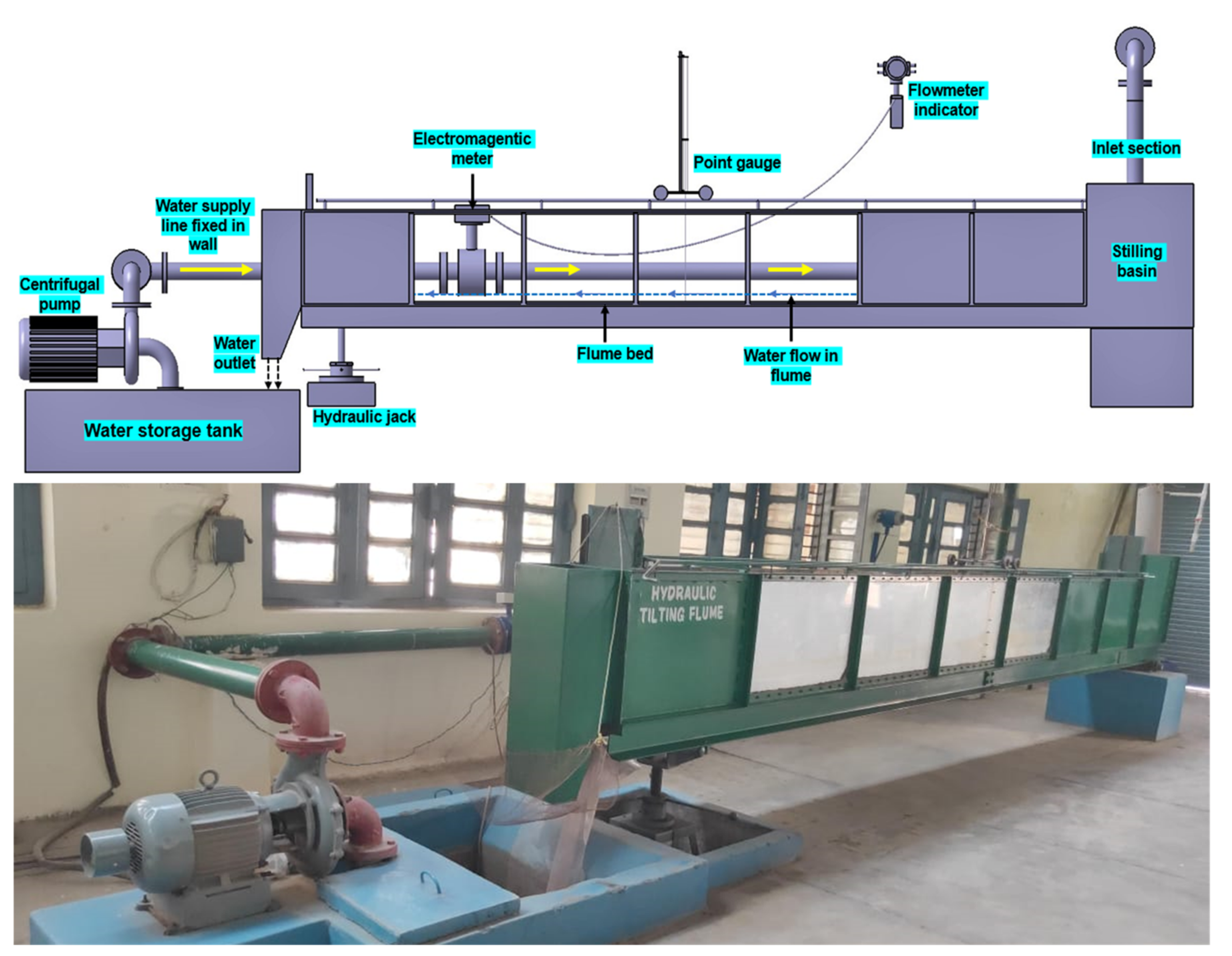
2.1. Experimental Setup and Data Observation

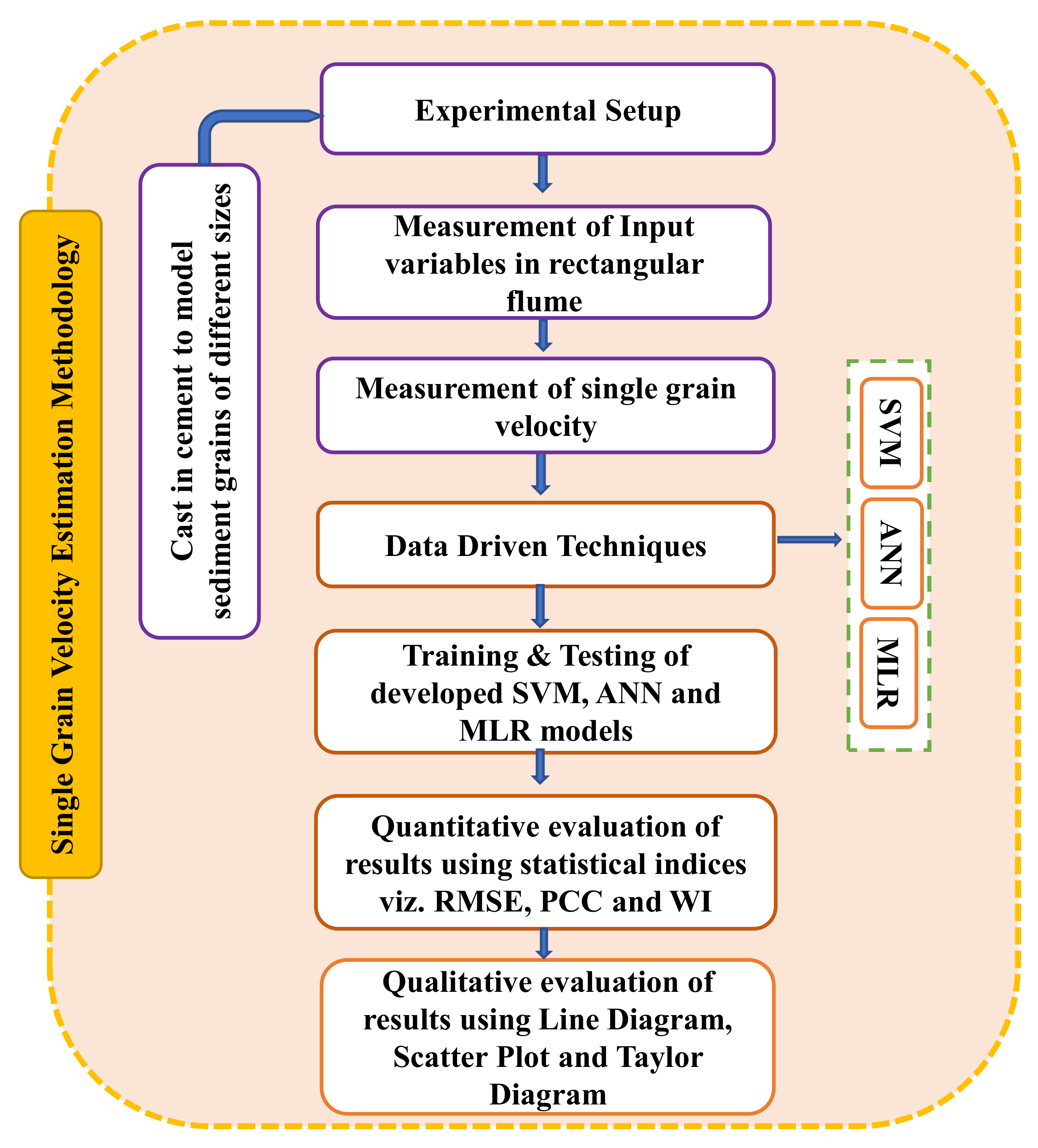
The experiments were carried out in a rectangular channel with a length of 7 m, a width of 0.30 m, and a depth of 0.60 m using three different sediment particles with (2 × 2 × 3) cm, (2 × 2 × 4) cm, and (3 × 3 × 4) cm. Figure 1 shows the experimental setup, with its different components used for conducting experiments. The particles were cast with cement mortar to model sediment grains of different sizes. The water was delivered by a centrifugal pump downstream of the flume and received from a water storage tank. Regulatory valves were placed on the flume’s water supply line-controlled discharge. A water flow meter was used to monitor the flow discharge. Flow depth was measured using a sophisticated point gauge mounted on the trolley for movement throughout the length of the flume. The flume channel was adjusted to the required bed slope with the help of the hydraulic screw jack provided in the mechanism.

A total of 108 experiments were conducted to determine grain velocity for three particle sizes, six discharges, and six-channel bed slopes. Experiments used six different discharges consisting of (12.8, 17.6, 23.2, 25.9, 29.6, and 33.6) L/s/m, while the channel bed slope changed from 1% to 4%. To achieve a fully developed flow, a grain particle of a specific size was put in a suitable position on the bed at 3.5 m from the flume’s upstream end. Attention was paid to avoiding turbulence and ensuring a steady flow along the channel’s length. A fixed span of 2.7 m length in the flume was considered for the particle’s movement. For every combination of experimental variables, flow depth, discharge, grain velocity, and the time took was recorded. Three times were, three replications performed to ensure precision in the observations.

2.1.1. Methodology

The present study focuses on establishing mathematical models using data-driven techniques to estimate single grain velocity based on the data generated using laboratory experiments. As discussed above, the experimental work was carried out in a rectangular hydraulic flume. Experimentally investigating single grain velocity in a rectangular channel flume was estimated and compared with different data-driven techniques, namely, support vector machine (SVM), artificial neural network (ANN), and multilinear regression (MLR) models. The developed models were evaluated using different performance indicators such as Pearson correlation coefficient (PCC), root mean square error (RMSE), Wilmot index, line diagram, scatter diagram, and Taylor diagram. Figure 2 describes the methodology used to estimate a single grain velocity in the study.

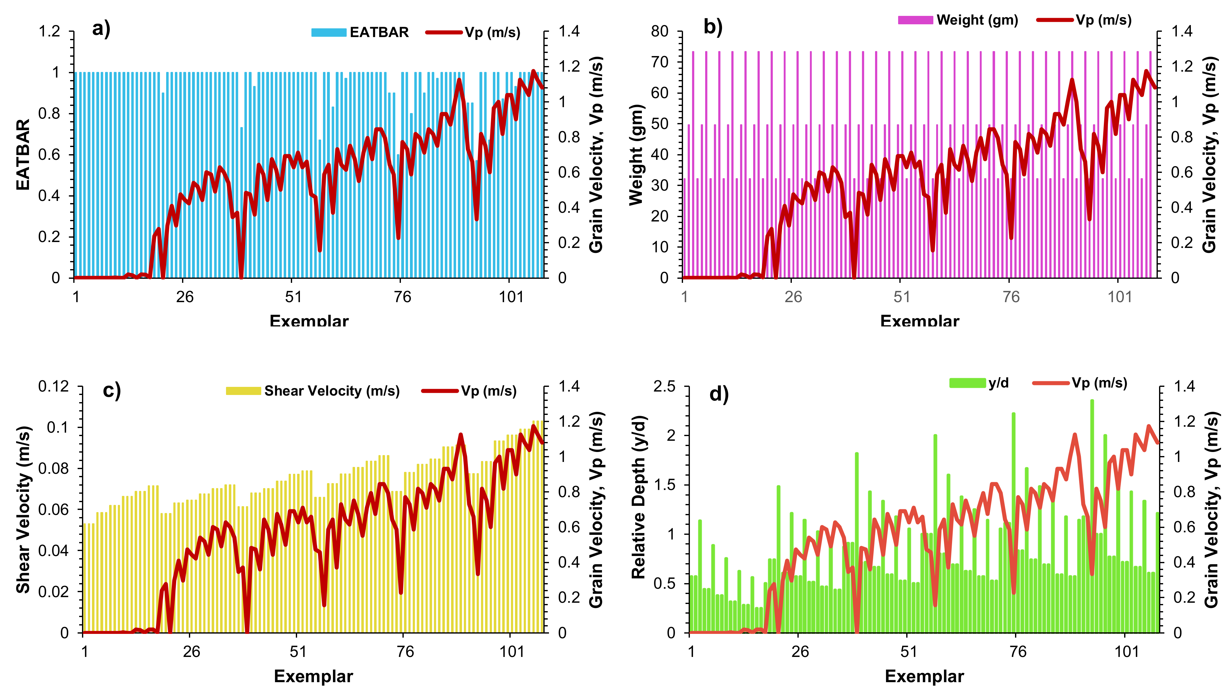
2.1.2. Input Parameters

EATBAR (λ) is the ratio of the exposed area (A_e) to the base area (A_b) of the particle, which changes with the change in the discharge and slope of the channel for the same particle and is calculated as

$$\mathrm{EATBAR} \left(\mathsf{\lambda }\right)=\frac{\mathrm{Ae}}{\mathrm{Ab}}$$

(1)

The shear velocity (U*) is evaluated by the following formula:

$$\mathrm{U}*=\sqrt{\mathrm{gRS}}$$

(2)

R represents the hydraulic radius in a section. S is the channel bed slope in fraction, and g is the gravitational acceleration.

Relative depth (y/d) is the ratio of flow depth to thickness (d).

The weight (W) is one of the fundamental parameters in sediment transport, which affects the particle’s movement. Due to varying submergence, the particle’s submerged weight also varies, altering the entire force dynamics for sediment transport.

2.2. Multiple Linear Regression—MLR

MLR stands for regression analysis, which involves more than one independent variable. The benefit of MLR is that it is straightforward, demonstrating how dependent and independent variables are related. The general form of the MLR model is:

$$\mathrm{Vp}= -3.284 + 1.935\mathsf{\lambda } - 0.008 \mathrm{W} + 25.953\mathrm{U}* + 0.503 (\mathrm{y}/\mathrm{d})$$

(3)

where $\mathrm{Vp}$ denotes the grain velocity (m/s), λ is EATBAR, W is the weight of the sediment particle, g, U* denotes the shear velocity (m/s), and y/d are the relative depth. These values are derived using the least square approach and reflect localized behavior, e.g., Kisi and Çobaner [36].

2.3. Artificial Neural Network—ANN

ANN is based on the training knowledge of the biological nervous system. It consists of several processing elements related to varying weights. The network consists of many layers of parallel processing elements called neurons. The most commonly used among ANN paradigms, the multilayer backpropagation network (MLP), was considered for this study. The MLP has a three-layered construction, namely, (a) an input layer, (b) a hidden layer, and (c) an output layer [37]. The input layer accepts data, handles it by the hidden layer, and shows the model’s results in the output layer. The input layer signals are dispersed to every hidden layer node depending on connection weights assigned between input (i.e., first layer) and hidden (i.e., middle) layers. These interconnection weights have been determined for respective inputs. In this present study, a hyperbolic tangent activation function (ranging from −1 to +1) was used as architecture for data normalization. Epoch = 1000 and threshold value = 0.001 were used to train the models based on trial-and-error methods. Each neuron in the middle and output layers receives the weighted sum of the previous layer’s output as input. The net output (NET_h) for layer j is given as:

$${\mathrm{NET}}_{\mathrm{h}}={{\displaystyle \sum }}_{\mathrm{n}=1}^{\mathrm{N}}\left({\mathrm{W}}_{\mathrm{ih}}{\mathrm{O}}_{\mathrm{pi}}+{\mathrm{b}}_{\mathrm{h}}\right)$$

(4)

where b_h represents the neuron threshold value for h, O_pi is the i-th output of the previous layer, and W_ih is the weight between the layers i and h. The Levenberg-Marquardt (LM) training algorithm was considered to adjust the weights for the current study.

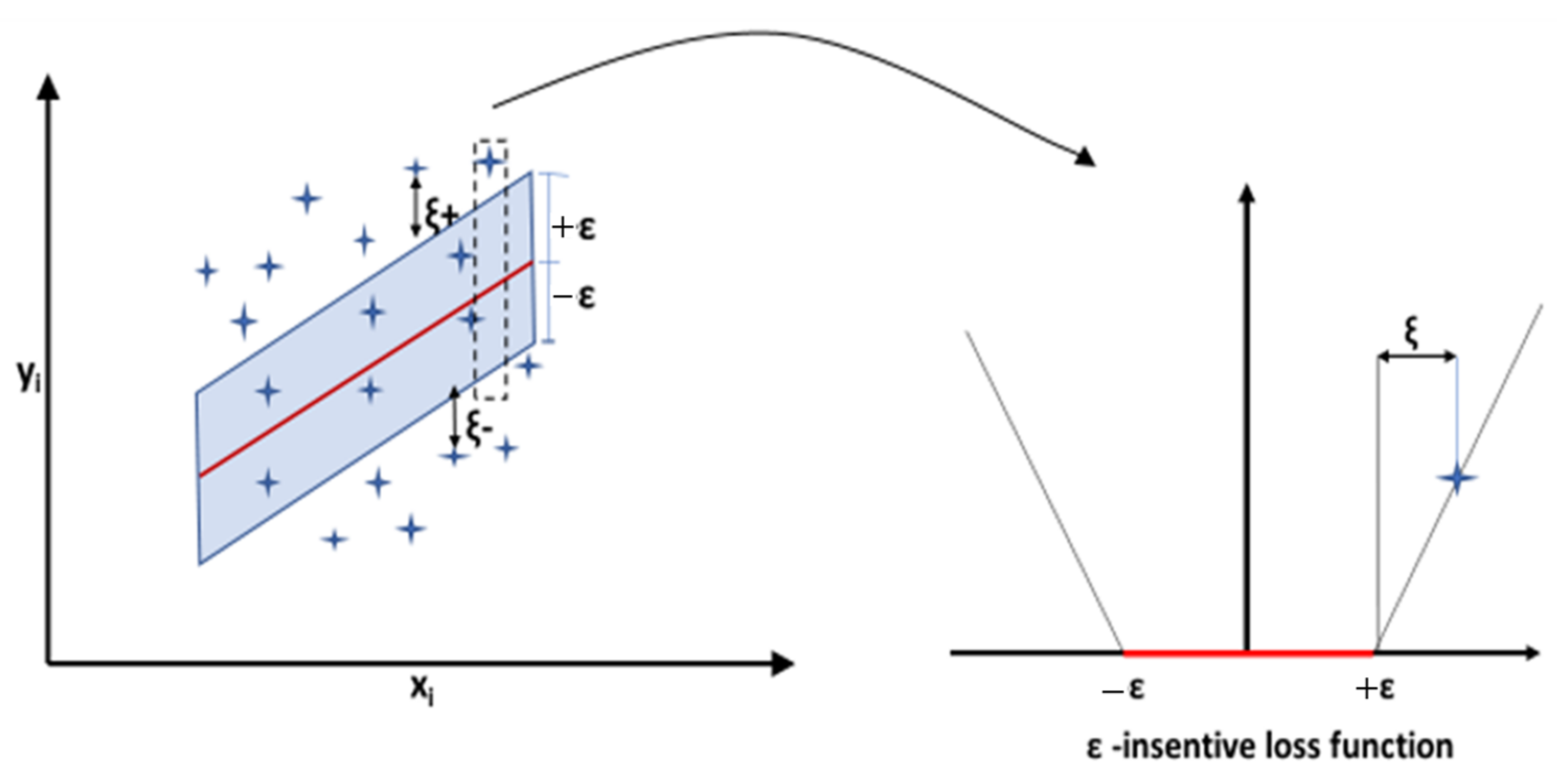
2.4. Support Vector Machine-SVM

SVM is a concept that was proposed by Vapnik [28]. The SVM technique finds a hyperplane between the input spaces. It disintegrates a given dataset and allows as much distance as close to both sides of the hyperplane to determine the points at which estimated errors are equal to and more significant than the so-called SVM tube scale. SVM techniques facilitate the development of a non-linear boundary by mapping the original input space to a higher-dimensional space. This dimensional space is called feature space. A kernel function characterizes this feature space mapping from a given input space. A penalty factor C is added for error classification to optimize this model. The cumulative penalty can be achieved by applying the penalties for each misclassification. As a result, the technique identifies a hyperplane that minimizes the margin and the total penalty. For optimization of the model, the combined penalty function is used as an objective function of the model. It has good generalization performance and is applicable in an approximation of both linear and non-linear datasets.

Considering a training dataset, T, represented as

T = (x₁, y₁), (x₂, y₂),…, (x_m, y_m)

(5)

where × X ⸦ ℝⁿ represents the training inputs, and y Y ⸦ ℝⁿ represents the training outputs. that a nonlinear function f(x) which is non-linear, is given by:

f (x) = w^TΦ(x_i) + b

(6)

where w represents the weight vector, b represents the bias, and Φ(x_i) denotes the high-dimensional feature space. Furthermore, data set T and, Equation (6) is transformed into Equation (7) as a constrained complex optimization problem stated as

Minimize: $\frac{1}{2}$w^Tw

$$\mathrm{subject} \mathrm{to}: \{y_i-\left({\mathrm{w}}^{\mathrm{T}}\mathsf{\Phi }\left({\mathrm{x}}_{\mathrm{i}}\right)+b\right)\le \epsilon y_i-\left({\mathrm{w}}^{\mathrm{T}}\mathsf{\Phi }\left({\mathrm{x}}_{\mathrm{i}}\right)+b\right)\ge \mathsf{\epsilon }$$

(7)

where ε (≥0) represents the maximum acceptable deviation.

Furthermore, the derived Equation for SVM is given in [15,38,39].

The final expansion of support vector regression is given by;

$$f(\mathrm{x})={\sum }_{i=1}^m\left({\alpha }_i^{+}-{\alpha }_i^{-}\right)K\left(x_i, x_j\right)+b$$

(8)

where, ${\alpha }_i^{+}$,${\alpha }_i^{-}$ are Lagrangian multipliers, and the term $K\left(x_i, x_j\right)$ is the kernel function. The kernel function allows for non-linear approximations. The kernel function used in the study was the linear kernel. The simplest type of kernel function is given as [40]:

$$K\left(x_i, x_j\right)=\left(x_i, x_j\right)$$

(9)

The three key parameters (kernel, C, $\mathsf{\gamma },$ and ε) on which the performance of SVM techniques depends (Figure 3).

However, the C and ε values influence the complexity of the final model for every specific kernel type. The parameters ε are responsible for regulating the number of support vectors. The values support vectors intuitively, when ε values are larger, lesser support vectors exit and thus lead to lower regression estimates. On the other side, the C value is essential in optimization. It represents the trade-off between the model’s sophistication and the degree of deviation. As a result, a higher C value reduces model complexity [42].

2.5. Performance Evaluation

Three performance criteria were used to evaluate the goodness of fit of the models in the present study. These are the root mean square error (RMSE), the Pearson correlation coefficient (PCC), and the Wilmot index (WI). The usage of RMSE, PCC, and WI offers a sufficient evaluation of each model’s performance. It compares the precision of the various trial and modeling methodologies employed in this work, further discussed by Ghorbani, Khatibi, Goel, FazeliFard and Azani [29], Kumar, Pandey, Sharma and Flügel [30], and Kumar et al., 2020.

$$\mathrm{RMSE}=\sqrt{\frac{{{\displaystyle \sum }}_{\mathrm{i}=1}^{\mathrm{N}}{\left({{\mathrm{V}}_{\mathrm{p}}}_{\mathrm{o}\mathrm{b}\mathrm{s},\mathrm{i}}-{{\mathrm{V}}_{\mathrm{p}}}_{\mathrm{p}\mathrm{r}\mathrm{e},\mathrm{i}}\right)}^2}{\mathrm{N}}}\hspace{1em}(0 \mathrm{to} \infty )$$

(10)

$$\mathrm{PCC}=\frac{{{\displaystyle \sum }}_{\mathrm{i}=1}^{\mathrm{N}}\left({{\mathrm{V}}_{\mathrm{p}}}_{\mathrm{obs},\mathrm{i}}-{{\overline{\mathrm{V}}}_{\mathrm{p}}}_{\mathrm{obs},\mathrm{i}}\right)\left({{\mathrm{V}}_{\mathrm{p}}}_{\mathrm{pre},\mathrm{i}}-{{\overline{\mathrm{V}}}_{\mathrm{p}}}_{\mathrm{pre},\mathrm{i}}\right)}{\sqrt{{{\displaystyle \sum }}_{\mathrm{i}=1}^{\mathrm{N}}{\left({{\mathrm{V}}_{\mathrm{p}}}_{\mathrm{obs},\mathrm{i}}-{{\overline{\mathrm{V}}}_{\mathrm{p}}}_{\mathrm{obs},\mathrm{i}}\right)}^2{{\displaystyle \sum }}_{\mathrm{i}=1}^{\mathrm{N}}{\left({{\mathrm{V}}_{\mathrm{p}}}_{\mathrm{pre},\mathrm{i}}-{{\overline{\mathrm{V}}}_{\mathrm{p}}}_{\mathrm{pre},\mathrm{i}}\right)}^2}}\hspace{1em}(-1 \mathrm{to} 1)$$

(11)

$$\mathrm{WI}=1-\frac{{{\displaystyle \sum }}_{\mathrm{i}=1}^{\mathrm{N}}{\left({{\mathrm{V}}_{\mathrm{p}}}_{\mathrm{o}\mathrm{b}\mathrm{s},\mathrm{i}}-{{\mathrm{V}}_{\mathrm{p}}}_{\mathrm{p}\mathrm{r}\mathrm{e},\mathrm{i}}\right)}^2}{{{\displaystyle \sum }}_{\mathrm{i}=1}^{\mathrm{N}}{(|{{\mathrm{V}}_{\mathrm{p}}}_{\mathrm{pre},\mathrm{i}}-{{\overline{\mathrm{V}}}_{\mathrm{p}}}_{\mathrm{obs},\mathrm{i}}|+|{{\overline{\mathrm{V}}}_{\mathrm{p}}}_{\mathrm{obs},\mathrm{i}}-{{\overline{\mathrm{V}}}_{\mathrm{p}}}_{\mathrm{obs},\mathrm{i}}|)}^2}\hspace{1em}(0 < \mathrm{WI} \le 1)$$

(12)

where, ${{\mathrm{V}}_{\mathrm{p}}}_{\mathrm{obs},\mathrm{i}}$ and ${{\mathrm{V}}_{\mathrm{p}}}_{\mathrm{pre},\mathrm{i}}$ are observed and predicted grain velocity of i-th observation, whereas, ${{\overline{\mathrm{V}}}_{\mathrm{p}}}_{\mathrm{obs},\mathrm{i}}$ and ${{\overline{\mathrm{V}}}_{\mathrm{p}}}_{\mathrm{pre},\mathrm{i}}$ are the average of the i-th observation, and N is the total number of observations.

3. Results and Discussion

As per the objectives of this study, the grain velocity was analyzed for several combinations of particle size, selected discharges, and channel slopes. To achieve these objectives, experiments were conducted on a hydraulic tilting flume in the laboratory. Three sizes of particles such as (2 × 2 × 3) cm, (2 × 2 × 4) cm, and (3 × 3 × 4) cm were used in this study. Six discharges of (12.8, 17.6, 23.2, 25.9, 29.6, and 33.6) L/s/m and bed slopes of 1, 1.5, 2, 2.5, 3 and 4% were considered for experimentation. The grain velocity with a particular orientation increased with channel slope and discharge but decreased with sediment particle weight. After critically analyzing the experimental results, four input parameters, shear velocity, EATBAR, relative depth, and particle weight, were selected as important variables to model grain velocity. Figure 4 and

Table 1. Statistical analysis of dependent (V_p) and independent variables (λ, W, U*, and y/d).

Variables	Mean	Median	Minimum	Maximum	Std. Dev.	C.V.	Skewness
All Data
λ	0.9707	1.000	0.5700	1.000	0.0823	0.0848	−3.283
W	51.733	49.60	32.200	73.40	16.966	0.32795	0.1874
U*	0.0754	0.0731	0.0529	0.1030	0.0120	0.1598	0.4072
y/d	0.8573	0.7142	0.2500	2.352	0.4281	0.4994	1.220
Vp	0.5473	0.600	0.0	1.174	0.3352	0.6124	−0.2776
Training Data
λ	0.9793	1.0	0.6	1.0	0.0706	0.0721	−3.964
W	51.476	49.6	32.2	73.4	17.035	0.3309	0.2091
U*	0.0696	0.0688	0.0529	0.0862	0.008	0.1150	0.0828
y/d	0.7894	0.6667	0.25	2.222	0.4031	0.5106	1.295
Vp	0.4070	0.474	0.0	0.8440	0.2793	0.6863	−0.3741
Testing Data
λ	0.9503	1.0	0.57	1.0	0.1035	0.1089	−2.368
W	52.344	49.6	32.2	73.4	17.05	0.3258	0.1369
U*	0.0892	0.0903	0.0774	0.103	0.0081	0.0914	0.1011
y/d	1.0185	0.8012	0.5714	2.352	0.4489	0.4407	1.1701
Vp	0.8806	0.8855	0.333	1.174	0.1901	0.2159	−0.6570

(Where λ = EATBAR, W = particle weight, U* = shear velocity, y/d = relative depth, V_p = grain velocity).

show the details of the observations from the experimentation. The shear velocity increased with discharge and channel slope for particular particle sizes. The shear velocity ranged from 0.0529 m/s to 0.1030 m/s. It was also observed that the EATBAR and relative depth values changed under three conditions first when there was a change in discharge, but the slope and particle size remained fixed; second, with a change in slope, but the other two variables remained fixed, and the third, when discharge and slope were fixed. However, the size of the sediment particle was changed. The EATBAR and relative depth values ranged from 0.57–1.00 and 0.25–2.35, respectively. When the sediment particle was fully submerged, i.e., particle height was less than the depth of flow of the particle. The exposed area and the base area remained the same. The value of EATBAR became 1.00, which was the maximum in this study. As depth flow decreased due to increased channel slope or decrease in discharge, the EATBAR value deviated from 1.0 due to a change in the exposed area.

In contrast, the base area remained the same. The grain velocity was maximum at 1.174 m/s for lighter weight particles of 32.2 gm, at 0.103 m/s shear velocity, 0.606 relative depth, and 1.0 EATBAR, at 4% channel bed slope and 33.6 L/s/m discharge, respectively. At the 1% slope of the channel bed, no movement in particles was observed in the discharge range of 12.8 L/s/m to 23.2 L/s/m. The movement in particles with a weight of 32.2 gm could be observed at a discharge of 25.9 L/s/m with 0.0033 m/s grain velocity.

3.1. Statistical Parameters

The statistical analysis of different independent variables, that is, EATBAR (λ), weight (gm), U* (m/s), y/d, and dependent variable V_p of all data, training, and testing sets included various statistical parameters such as mean, median, minimum and maximum value, standard deviation, CV and skewness. These statistical parameters showed data heterogeneity over the whole time series. Cross-validating is essential for the same statistical population if the data is divided into training and test subsets. Due to the high skewness, the model’s efficiency was adversely affected. The standard deviation values suggest that the values are farther from zero, indicating that the data heterogeneity is more significant. The mean value variance is greater (Table 1).

3.2. Trial Selection

MLR, ANN, and SVM were analyzed in two phases to select the best model: the training and testing phases. The performance was evaluated based on the lower value of RMSE (0: +: satisfactory: unsatisfactory), the higher value of PCC, and WI (close to +1) for selections of the best model. Several trials were performed on a single output in the best model selection process for ANN and SVM. The best trials of the developed models during the training and testing phases are presented in

Table 2. During the training and testing phase, performance evaluations of MLR, ANN, and SVM models.

Model	Training			Testing
	RMSE (m/s)	PCC	WI	RMSE (m/s)	PCC	WI
MLR	0.1340	0.8756	0.7532	0.1459	0.8375	0.6789
ANN
Trial-1	0.1266	0.8911	0.8106	0.3109	0.1509	0.3420
Trial-2	0.0873	0.9502	0.8756	0.2154	0.3636	0.4579
Trial-3	0.0689	0.9692	0.8799	0.1721	0.5176	0.5012
Trial-4	0.0663	0.9728	0.8999	0.2302	0.1945	0.3666
Trial-5	0.0699	0.9678	0.8916	0.1906	0.4365	0.4751
Trial-6	0.0759	0.9625	0.9439	0.1821	0.4900	0.5058
SVM
Trial-1	0.1423	0.8595	0.7475	0.1208	0.8852	0.7231
Trial-2	0.1381	0.8675	0.7531	0.1341	0.8688	0.7022
Trial-3	0.1431	0.8577	0.7479	0.1195	0.8877	0.7243
Trial-4	0.1408	0.8622	0.7513	0.1247	0.8795	0.7150

. Trial-3 of both ANN and SVM, respectively, given in Table 2, were more promising than the other trials for the combination.

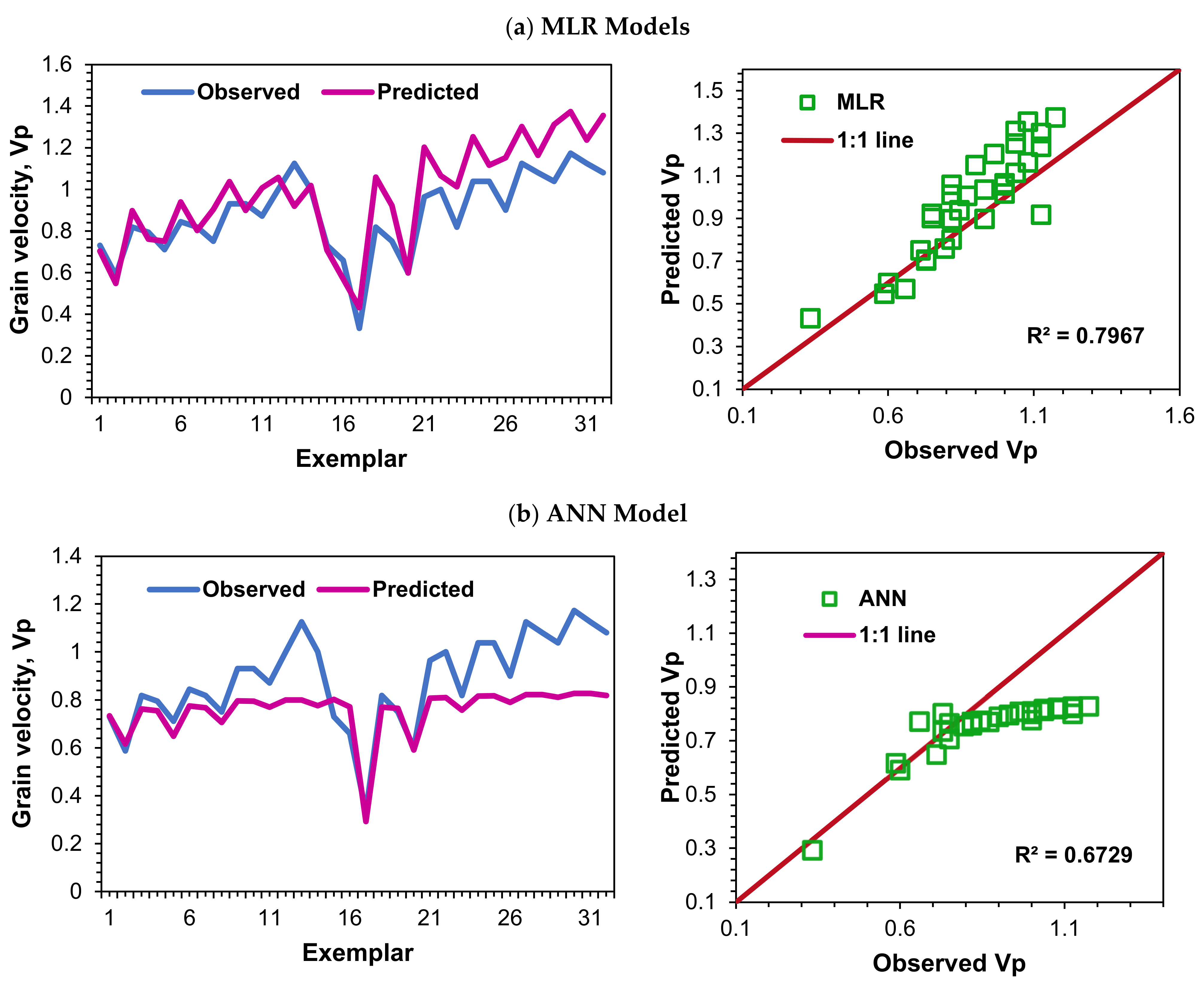
3.3. Quantitative Performance Evaluation

After considering the three techniques for best tests (Table 2), the values of the RMSE, PCC, and WI values of the MLR techniques for the training phase were obtained as 0.1340, 0.8756, and 0.7532; respectively, while for the testing phase, these values were 0.1459, 0.8375, and 0.6789. In the ANN-based model, the value of RMSE was obtained in the range of 0.0663 to 0.1266, and PCC was obtained in the range of 0.8911 to 0.9728. In contrast, WI was obtained in the range of 0.8106 to 0.8999 during the training phase. During the testing phase in the RMSE ANN model, the value was obtained in the range of 0.1721 to 0.3109, and PCC was observed to be in the range of 0.1509 to 0.5176. In contrast, WI was observed in the range of 0.3420 to 0.5012. The results of the ANN model did not improve when the number of layers in the hidden layer was increased to two (Trial 5) and three (Trial 6). The performance indices in SVM techniques were as RMSE ranged from 0.1381 to 0.1431, PCC ranged from 0.8577 to 0.8675, and WI ranged from 0.7475 to 0.7531 training phase. In contrast, in the testing phase of the SVM techniques, the value of RMSE was obtained in the range of 0.1195 to 0.1341, PCC was in the range of 0.8688 to 0.8877, and WI was observed in the range of 0.7022 to 0.7243. The architecture used for all developed ANN and SVM models is shown in

Table 3. The architecture used for the development of ANN and SVM models.

Model/Trial	Architecture
ANN
Trial-1	4-1-1
Trial-2	4-4-1
Trial-3	4-5-1
Trial-4	4-7-1
Trial-5	4-5-5-1
Trial-6	4-4-4-4-1
SVM
Trial-1	C = 10, $\mathsf{\gamma }$ = 0.25, ε = 0.01
Trial-2	C = 10, $\mathsf{\gamma }$ = 0.25, ε = 0.1
Trial-3	C = 10, $\mathsf{\gamma }$ = 0.45, ε = 0.01
Trial-4	C = 10, $\mathsf{\gamma }$ = 0.45, ε = 0.05

.

Based on the values of the performance indices during the testing phase of the models developed using three different techniques, the values of RMSE were obtained as SVM (0.1195) > MLR (0.1459) > ANN (0.1721). The values of PCC were obtained as SVM (0.8877) > MLR (0.8375) > ANN (0.5176) of the values was obtained as SVM (0.7243) > MLR (0.6789) > ANN (0.5012). Thus, the overall comparison of performance indicators for these models revealed that the model’s performance based on the SVM technique was the best. In contrast, the model’s performance developed using ANN was the worst. To assess the dissimilarity among the results obtained from various models, a t-test was performed, which provided the p-value of these three models (P = 1.11 × 10⁻⁶ for ANN, P = 6.34 × 10⁻⁵ for MLR, and P = 9.4 × 10⁻⁵ for SVM), which is less than 0.05 and suggested that there is a significant difference between observed and predicted mean values of grain velocity in all three models. The observed mean values of grain velocity were 0.8806 m/s. They predicted that the mean grain velocity was 0.7565 m/s, 0.970815 m/s, and 0.9529 m/s for the ANN, MLR, and SVM models. Thus, the mean absolute difference between observed and predicted grain velocities was 0.1240 for ANN, 0.09019 for MLR, and 0.07236 for SVM. Therefore, it is confirmed that the SVM-based model predicted close to the corresponding observed values than MLR and ANN-based models. The Friedman test also verified a significant (p < 0.05) difference between observed and predicted grain velocity in MLR, ANN, and SVM models.

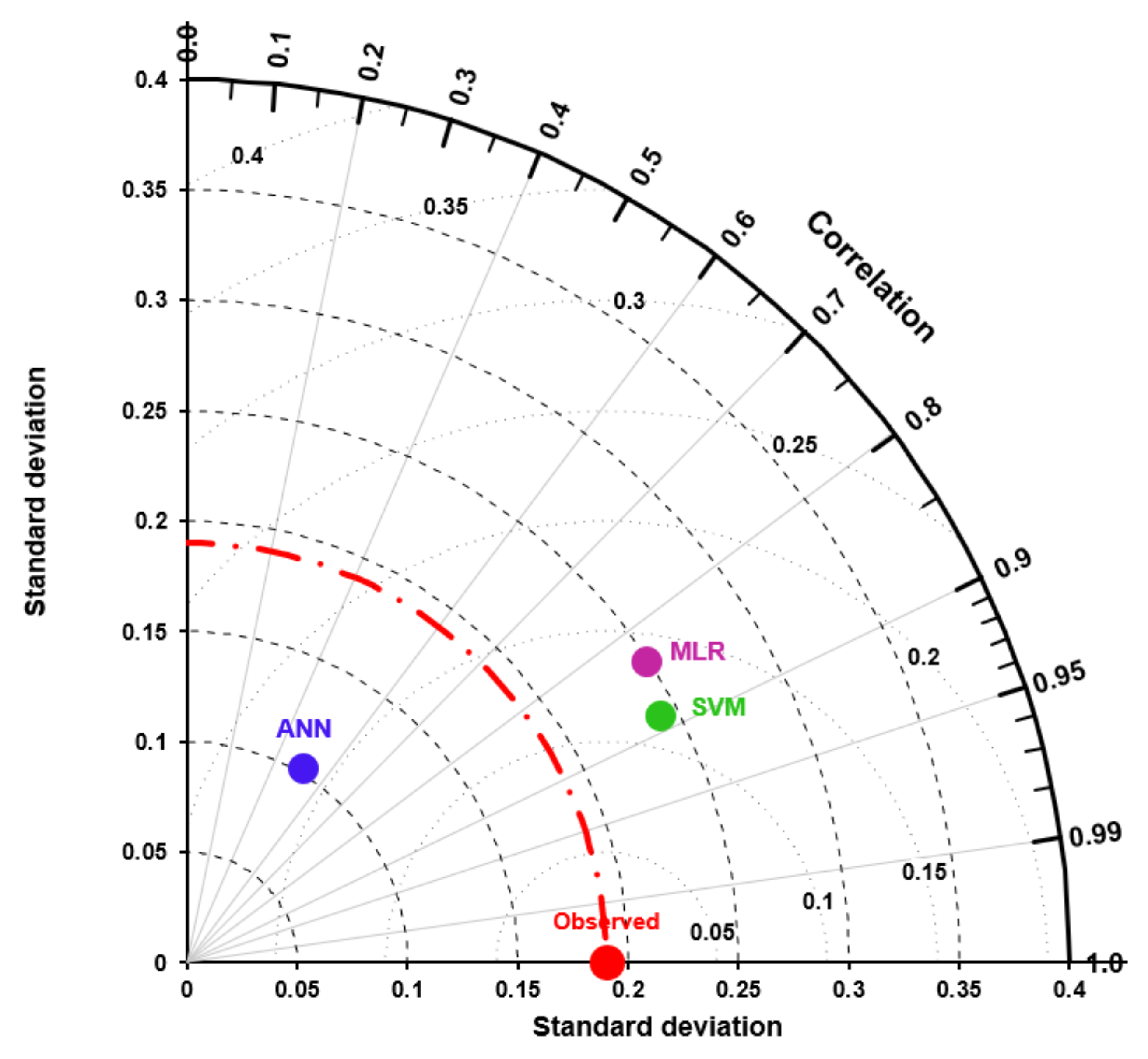
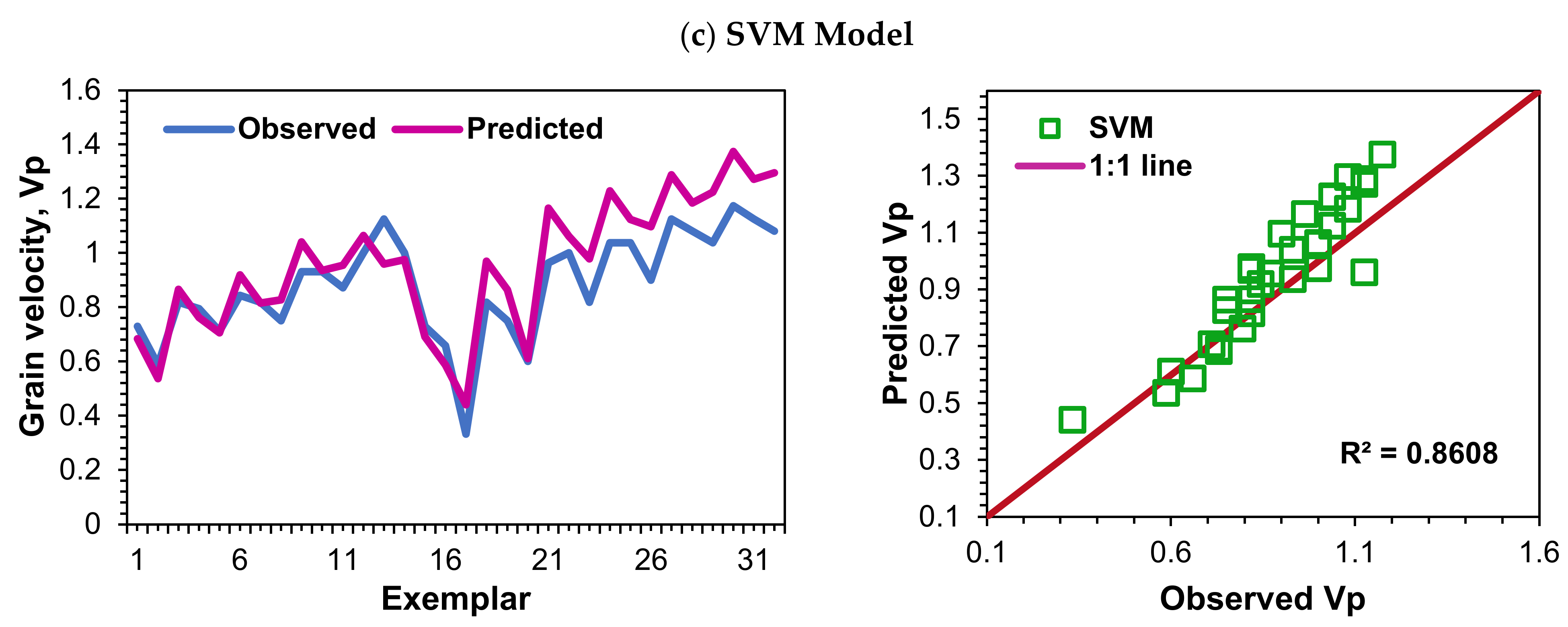
3.4. Qualitative Performance Evaluation

To assess the qualitative performance of these models, the observed data was plotted with the model estimated data of the model, as shown in Figure 5. These plots revealed that the developed models slightly over-predicted higher grain velocity in MLR and SVM-based models. In contrast, the grain velocity was underpredicted in the entire range in the ANN-based model variation. The values of the coefficient of determination (R²) were highest (0.8608) for the SVM model, and the lowest value (0.6729) was obtained for the ANN-based model. The value of (R²) was 0.7967 in the case of the MLR-based model.

Taylor diagrams (Figure 6) indicated that although the model correlation was satisfactory, it was highest in the case of SVM and lowest in the case of ANN. As another comprehensive graphical presentation, a Taylor diagram compared the observed and predictive values using three statistical parameters: the CC, the root mean square difference (RMSD), and the standard deviation. The best model is the one that has less distance to the observed point [30,43].

From Taylor diagrams (Figure 6), the order of correlation value from best to worst was the same as explained earlier, i.e., SVM (0.9277) > MLR (0.8926) > ANN (0.8203). The standard deviation value for the observed data was obtained as 0.1901. The MLR, ANN, and SVM model predicted values; the standard deviation was 0.2487, 0.1025, and 0.2419, respectively. Therefore, the deviation between observed and model-predicted values was lowest (0.0518) for the SVM technique, followed by MLR- (0.0586) and ANN- (0.0876) based models. Thus, from a qualitative evaluation of observed data and predicted data using different techniques, it was found that the SVM technique performed better, followed by the MLR and then ANN techniques. Based on this analysis, it thus could be inferred in terms of the input parameters such as EATBAR, weight, shear velocity, and relative depth; the model developed using the support vector machine technique was superior for predicting single grain velocity compared to the models developed using ANN and MLR techniques.

Further, the MLR-based model better predicted the performance of single grain velocity than the model developed using the ANN technique. Previous studies on the simulation of experimental data have been made in Kumari [44], which integrates the soft computing techniques with experimental results to estimate post-fire bond behavior. The bond strength and bond-slip behavior have been estimated using gene expression programming (GEP) and the ANN. The ANN has a significant positive association with experimental results and makes more precise predictions than the investigated codes. Further, Sheikh Khozani, Safari, Danandeh Mehr and Wan Mohtar [24] developed incipient sediment motion models with ensemble genetic programming in rectangular form. The new models incorporate dimensionless input factors such as relative particle size, relative deposited bed thickness, channel friction factor, and channel bed slope to evaluate the particle Froude number in rectangular channels. It was revealed that the combined use of fluid, flow, sediment and channel characteristics was superior in estimating incipient motion. Earlier, Wan Mohtar, Afan, El-Shafie, Bong, and Ab. Ghani [27] estimated incipient sediment motion by the effects of bed deposits in sewers using ANN. For predicting the motion of sediment, feed-forward neural network (FFNN) and radial basis function (RBF) were two algorithms of ANN employed to predict the critical velocity over varying sediment thickness, median grain size, and water depth. Thus, soft computing techniques have been an effective tool for simulating experimental data.

4. Conclusions

The experimental results showed that the grain velocity increased with an increase in channel slope and discharge but decreased with sediment particle weight. The models developed to simulate the output parameter, grain velocity in input parameters such as the exposed area to base area ratio, relative depth, shear velocity, and particle weight using SVM, ANN, and MLR techniques were developed to predict grain velocity. However, based on the prediction performance in terms of statistical indices, namely, RMSE, PCC, and WI, the SVM technique-based model with RMSE = 0.1195, PCC = 0.8877. WI = 0.7243 was found to be the best. The lowest prediction performance was obtained for the ANN technique’s model. Similar findings were obtained with the scatter plot and Taylor diagram.

References

1. Chien, N.; Wan, Z. Mechanics of Sediment Transport; American Society of Civil Engineers (ASCE): Reston, VA, USA, 1999. [Google Scholar]
2. Van Rijn, L.C. Sediment Transport, Part I: Bed Load Transport. J. Hydraul. Eng. 1984, 110, 1431–1456. [Google Scholar] [CrossRef] [Green Version]
3. Van Rijn, L.C. Sediment Transport, Part II: Suspended Load Transport. J. Hydraul. Eng. 1984, 110, 1613–1641. [Google Scholar] [CrossRef]
4. Gomez, B.; Church, M. An assessment of bed load sediment transport formulae for gravel bed rivers. Water Resour. Res. 1989, 25, 1161–1186. [Google Scholar] [CrossRef]
5. Zhang, X.-D. Machine Learning. In A Matrix Algebra Approach to Artificial Intelligence; Zhang, X.-D., Ed.; Springer Singapore: Singapore, 2020; pp. 223–440. [Google Scholar]
6. Safari, M.J.S.; Arashloo, S.R. Kernel ridge regression model for sediment transport in open channel flow. Neural Comput. Appl. 2021, 33, 11255–11271. [Google Scholar] [CrossRef]
7. Novak, P.; Nalluri, C. Incipient Motion of Sediment Particles Over Fixed Beds. J. Hydraul. Res. 1984, 22, 181–197. [Google Scholar] [CrossRef]
8. Tabarestani, M.K.; Zarrati, A.R. Sediment transport during flood event: A review. Int. J. Environ. Sci. Technol. 2015, 12, 775–788. [Google Scholar] [CrossRef] [Green Version]
9. Papanicolaou, A.N.; Knapp, D.; Strom, K. Bedload Predictions by Using the Concept of Particle Velocity: Applications. In Hydraulic Measurements and Experimental Methods 2002; American Society of Civil Engineers: Reston, VA, USA, 2002; pp. 1–10. Available online: https://www.researchgate.net/publication/299813875_Bedload_Predictions_by_Using_the_Concept_of_Particle_Velocity_Applications (accessed on 12 March 2022).
10. Julien, P.Y.; Bounvilay, B. Velocity of Rolling Bed Load Particles. J. Hydraul. Eng. 2013, 139, 177–186. [Google Scholar] [CrossRef]
11. Cheng, N.-S.; Emadzadeh, A. Average Velocity of Solitary Coarse Grain in Flows over Smooth and Rough Beds. J. Hydraul. Eng. 2014, 140, 04014015. [Google Scholar] [CrossRef]
12. Frey, P. Particle velocity and concentration profiles in bedload experiments on a steep slope. Earth Surf. Process. Landf. 2014, 39, 646–655. [Google Scholar] [CrossRef]
13. Nourani, V.; Hosseini Baghanam, A.; Adamowski, J.; Kisi, O. Applications of hybrid wavelet–Artificial Intelligence models in hydrology: A review. J. Hydrol. 2014, 514, 358–377. [Google Scholar] [CrossRef]
14. Demirci, M.; Baltaci, A. Prediction of suspended sediment in river using fuzzy logic and multilinear regression approaches. Neural Comput. Appl. 2013, 23, 145–151. [Google Scholar] [CrossRef]
15. Misra, D.; Oommen, T.; Agarwal, A.; Mishra, S.K.; Thompson, A.M. Application and analysis of support vector machine based simulation for runoff and sediment yield. Biosyst. Eng. 2009, 103, 527–535. [Google Scholar] [CrossRef]
16. Kakaei Lafdani, E.; Moghaddam Nia, A.; Ahmadi, A. Daily suspended sediment load prediction using artificial neural networks and support vector machines. J. Hydrol. 2013, 478, 50–62. [Google Scholar] [CrossRef]
17. Meshram, S.G.; Singh, V.P.; Kisi, O.; Karimi, V.; Meshram, C. Application of Artificial Neural Networks, Support Vector Machine and Multiple Model-ANN to Sediment Yield Prediction. Water Resour. Manag. 2020, 34, 4561–4575. [Google Scholar] [CrossRef]
18. Jain, S.K.; Chalisgaonkar, D. Setting Up Stage-Discharge Relations Using ANN. J. Hydrol. Eng. 2000, 5, 428–433. [Google Scholar] [CrossRef]
19. Garbrecht, J.D. Comparison of Three Alternative ANN Designs for Monthly Rainfall-Runoff Simulation. J. Hydrol. Eng. 2006, 11, 502–505. [Google Scholar] [CrossRef] [Green Version]
20. Mukerji, A.; Chatterjee, C.; Raghuwanshi, N.S. Flood Forecasting Using ANN, Neuro-Fuzzy, and Neuro-GA Models. J. Hydrol. Eng. 2009, 14, 647–652. [Google Scholar] [CrossRef]
21. Rajaee, T.; Nourani, V.; Zounemat-Kermani, M.; Kisi, O. River Suspended Sediment Load Prediction: Application of ANN and Wavelet Conjunction Model. J. Hydrol. Eng. 2011, 16, 613–627. [Google Scholar] [CrossRef]
22. Ab Ghani, A.; Azamathulla, H.M. Development of GEP-based functional relationship for sediment transport in tropical rivers. Neural Comput. Appl. 2014, 24, 271–276. [Google Scholar] [CrossRef]
23. Bhattacharya, B.; Price, R.K.; Solomatine, D.P. Machine Learning Approach to Modeling Sediment Transport. J. Hydraul. Eng. 2007, 133, 440–450. [Google Scholar] [CrossRef]
24. Sheikh Khozani, Z.; Safari, M.J.S.; Danandeh Mehr, A.; Wan Mohtar, W.H.M. An ensemble genetic programming approach to develop incipient sediment motion models in rectangular channels. J. Hydrol. 2020, 584, 124753. [Google Scholar] [CrossRef]
25. Mehr, A.D.; Safari, M.J.S. Application of Soft Computing Techniques for Particle Froude Number Estimation in Sewer Pipes. J. Pipeline Syst. Eng. Pract. 2020, 11, 04020002. [Google Scholar] [CrossRef]
26. Montes, C.; Berardi, L.; Kapelan, Z.; Saldarriaga, J. Predicting bedload sediment transport of non-cohesive material in sewer pipes using evolutionary polynomial regression–multi-objective genetic algorithm strategy. Urban Water J. 2020, 17, 154–162. [Google Scholar] [CrossRef] [Green Version]
27. Wan Mohtar, W.H.M.; Afan, H.; El-Shafie, A.; Bong, C.H.J.; Ab Ghani, A. Influence of bed deposit in the prediction of incipient sediment motion in sewers using artificial neural networks. Urban Water J. 2018, 15, 296–302. [Google Scholar] [CrossRef]
28. Vapnik, V.N. An overview of statistical learning theory. IEEE Trans. Neural Netw. 1999, 10, 988–999. [Google Scholar] [CrossRef] [Green Version]
29. Ghorbani, M.A.; Khatibi, R.; Goel, A.; FazeliFard, M.H.; Azani, A. Modeling river discharge time series using support vector machine and artificial neural networks. Environ. Earth Sci. 2016, 75, 685. [Google Scholar] [CrossRef]
30. Kumar, D.; Pandey, A.; Sharma, N.; Flügel, W.-A. Daily suspended sediment simulation using machine learning approach. Catena 2016, 138, 77–90. [Google Scholar] [CrossRef]
31. Rahgoshay, M.; Feiznia, S.; Arian, M.; Hashemi, S.A.A. Modeling daily suspended sediment load using improved support vector machine model and genetic algorithm. Environ. Sci. Pollut. Res. 2018, 25, 35693–35706. [Google Scholar] [CrossRef] [PubMed]
32. Einstein, H.A. The Bed-Load Function for Sediment Transportation in Open Channel Flows; US Government Printing Office: Washington, DC, USA, 1950; p. 71. [Google Scholar]
33. Fernandez Luque, R.; Van Beek, R. Erosion And Transport Of Bed-Load Sediment. J. Hydraul. Res. 1976, 14, 127–144. [Google Scholar] [CrossRef] [Green Version]
34. Abbott, J.E.; Francis, J.R.D.; Owen, P.R. Saltation and suspension trajectories of solid grains in a water stream. Philos. Trans. R. Soc. Lond. Ser. A Math. Phys. Sci. 1977, 284, 225–254. [Google Scholar] [CrossRef]
35. Bridge, J.S.; Dominic, D.F. Bed Load Grain Velocities and Sediment Transport Rates. Water Resour. Res. 1984, 20, 476–490. [Google Scholar] [CrossRef]
36. Kisi, Ö.; Çobaner, M. Modeling River Stage-Discharge Relationships Using Different Neural Network Computing Techniques. Clean Soil Air Water 2009, 37, 160–169. [Google Scholar] [CrossRef]
37. Rajaee, T.; Mirbagheri, S.A.; Zounemat-Kermani, M.; Nourani, V. Daily suspended sediment concentration simulation using ANN and neuro-fuzzy models. Sci. Total Environ. 2009, 407, 4916–4927. [Google Scholar] [CrossRef]
38. Hipni, A.; El-shafie, A.; Najah, A.; Karim, O.A.; Hussain, A.; Mukhlisin, M. Daily Forecasting of Dam Water Levels: Comparing a Support Vector Machine (SVM) Model With Adaptive Neuro Fuzzy Inference System (ANFIS). Water Resour. Manag. 2013, 27, 3803–3823. [Google Scholar] [CrossRef]
39. Gholami, R.; Fakhari, N. Chapter 27-Support Vector Machine: Principles, Parameters, and Applications. In Handbook of Neural Computation; Samui, P., Sekhar, S., Balas, V.E., Eds.; Academic Press: Cambridge, MA, USA, 2017; pp. 515–535. [Google Scholar]
40. Han, D.; Chan, L.; Zhu, N. Flood forecasting using support vector machines. J. Hydroinformatics 2007, 9, 267–276. [Google Scholar] [CrossRef]
41. Lin, J.-Y.; Cheng, C.-T.; Chau, K.-W. Using support vector machines for long-term discharge prediction. Hydrol. Sci. J. 2006, 51, 599–612. [Google Scholar] [CrossRef]
42. Cherkassky, V.; Ma, Y. Practical selection of SVM parameters and noise estimation for SVM regression. Neural Netw. 2004, 17, 113–126. [Google Scholar] [CrossRef] [Green Version]
43. Sharafati, A.; Haghbin, M.; Haji Seyed Asadollah, S.B.; Tiwari, N.K.; Al-Ansari, N.; Yaseen, Z.M. Scouring Depth Assessment Downstream of Weirs Using Hybrid Intelligence Models. Appl. Sci. 2020, 10, 3714. [Google Scholar] [CrossRef]
44. Kumari, A. Effect of Sediment Particle Orientation on its Movement under Varying Channel Slope and Discharge Conditions. Master’s Thesis, GB Pant University of Agriculture and Technology, Pantnagar, India, 2017. [Google Scholar]
Figure 1. Experimental setup of the hydraulic flume; schematic presentation (top part) and lab view (lower part).
Water 14 01325 g001
Figure 2. Flow diagram for single grain velocity estimation.
Water 14 01325 g002
Figure 3. Soft margin loss setting for a linear SVM and ε-insentive loss function adapted after Lin et al. [41].
Water 14 01325 g003
Figure 4. Plots of the dependent variable Vp (m/s) and input variable: (a) EATBAR, (b) weight (gm), (c) shear velocity (m/s), (d) relative depth.
Water 14 01325 g004
Figure 5. Observed versus predicted grain velocity by the (a) MLR, (b) ANN, and (c) SVM models during the testing phase.
Water 14 01325 g005aWater 14 01325 g005b
Figure 6. Taylor diagram of MLR, ANN, and SVM corresponding to observed grain velocity (Vp).
Water 14 01325 g006