A Hybrid Prediction Framework for Water Quality with Integrated W-ARIMA-GRU and LightGBM Methods

Abstract

Water is the source of life, and in recent years, with the progress in technology, water quality data have shown explosive growth; how to use the massive amounts of data for water quality prediction services has become a new opportunity and challenge. In this paper, we use the surface water quality data of an area in Beijing collected and compiled by Zhongguancun International Medical Laboratory Certification Co., Ltd. (Beijing, China). On this basis, we decompose the original water quality indicator data series into two series in terms of trend and fluctuation; for the characteristics of the decomposed series data, we use the traditional time series prediction method to model the trend term, introduce the deep learning method to interpret the fluctuation term, and fuse the final prediction results. Compared with other models, our proposed integrated Wavelet decomposition, Autoregressive Integrated Moving Average (ARIMA) and Gated Recurrent Unit (GRU) model, which is abbreviated as the W-ARIMA-GRU model, has better prediction accuracy, stability, and robustness for three conventional water quality indicators. At the same time, this paper uses the ensemble learning model LightGBM for the prediction of water quality evaluation level, and the accuracy and F1-score reached 97.5% and 97.8%, respectively, showing very strong performance. This paper establishes a set of effective water quality prediction frameworks that can be used for timely water quality prediction and to provide a theoretical model and scientific and reasonable analysis reference for the relevant departments for advanced control.

1. Introduction

Water is the source of life and is an important basis for ecological cycles and social activities. Water quality is defined by a combination of physical, chemical, and biological parameters contained within water resources. It is critical to determine the quality of water resources before they are used for various intended uses, such as drinking, agriculture, recreation, and industry. However, in recent years, numerous paths to economic benefit have resulted in harm to the environment [1], and many countries around the world have seen their limited freshwater resources decrease dramatically with rapid economic development. Water pollution has become a serious problem, presenting one of the great obstacles to human health as well as sustainable development. For example, although China has 2.8 trillion m³ in water resources [2], its per capita share of water resources is only 2400 m³ due to its huge population [3], which accounts for less than a quarter of the world’s total per capita water resources. Domestic sewage as well as industrial wastewater are discharged into water bodies without treatment, which leads to serious damage to the environment [4]. On the other hand, with the progress of technology, water quality data have shown explosive growth; the use of the massive amounts of data with the development of various new technologies such as machine learning and artificial neural networks has also provided new solutions to surface water management problems. Therefore, this paper will use conventional water quality indicators and neural network methods for the prediction of watershed water quality research, in order to be able to prevent water quality deterioration in a timely manner, to enable the relevant departments to provide theoretical models and a scientific and reasonable analysis of references for prevention and control.

In recent years, the main methods for water quality simulation and prediction have been regression analysis, time series models, and artificial neural networks.

Regression analysis model is used because water quality parameters have different degrees of correlation; the model allows for choosing the significant correlation parameters for mutual estimation according to the known correlation estimates for prediction and analysis. Zhang et al. [5] proposed a multilevel regression method to predict baseflow indicators. The experimental results showed that the multilevel regression method helped to improve the prediction performance of the baseflow indicators. Kadkhodazadeh et al. used six machine learning techniques for prediction and uncertainty analysis of reference evapotranspiration (ETo) at nine sites in two basins, Lake Urmia and Sefidrood, for the period 2021–2050, using the LSBoost model for ETo prediction under climate change. The results showed that ETo increased at all stations [6]. Ewaid et al. developed a multiple linear regression model based on the specified weights and predicted the water quality of the Euphrates River [7]. Qin et al. integrated a particle swarm algorithm as well as a support vector regression machine approach to predict water quality in Yixing, China, and the model showed a strong performance [8]. Kadkhodazadeh et al. proposed a novel least square support vector machine (LSSVM) model and gradient-based optimizer (GBO) algorithm to evaluate water quality (WQ) parameters using data from three sites in the Karun River basin—Ahvaz, Armand, and Gotvand—and they developed and experimented with conductivity (EC) and total dissolved solids (TDS) models. The accuracy of the proposed hybrid model was found to be higher than that of models such as artificial neural network [9].

A time series analysis model expresses the variation pattern of water quality parameters by analyzing the long-term trends, random variables, and periodic trends of water quality data, combined with the stochastic perturbation of data and autocorrelation of lagged terms. Elhag et al. [10] used a seasonal ARIMA model to predict the water quality remote sensing data in Saudi Arabia. Experiments showed that the model was efficient in predicting data within six months. Lv et al. [11] monitored and studied river water quality, algal density, and algal community and used an ARIMA model to simulate algal density in reclaimed water recharge rivers. Wang et al. used the Holt-Winters seasonal ARIMA model to predict water quality indicators such as total phosphorus and total nitrogen in a reservoir with a prediction accuracy of no less than 97.5% [12]. Tizro et al. used an ARIMA model to predict nine water quality parameters in the Hor Rood River, and the model showed an unimpressive performance [13].

The artificial neural network model has become an important method for water quality prediction; after continuous improvement and innovation, the speed and accuracy of water quality prediction have also improved. Jung et al. [14] explored the use of an artificial neural network (ANN) model to predict the river nitrate load problem and load prediction of five major river waters in Midwestern USA and obtained a good prediction effect. Archana et al. used deep belief networks in unsupervised learning to study pH, dissolved oxygen, turbidity, and other water quality parameters in the Chaskaman reservoir for prediction and analysis [15]. The results showed that the method outperformed the classical prediction methods. Wu et al. [16] proposed, based on an adaptive learning rate, a BP neural network algorithm water quality prediction model, successfully applied to the urban water supply system in Oslo and Bergen, Norway; the management of the two cities’ water supply systems provided a reference. Hameed et al. used two artificial neural network models (RBFNN and BPNN) for the prediction of water quality in Malaysia. Both models performed well, but the RBFNN model was superior in terms of prediction accuracy [17]. Wei et al. [18] combined a cereal bird search and radial basis (RBF) neural network and classified the water quality of surface water in Zhejiang province. The experimental results showed that the method had a higher accuracy of water quality classification than a feedback neural network (back propagation, BP) and an RBF neural network based on gradient descent and a genetic algorithm. Hu and Liu et al. [19,20] used LSTM to study seawater quality in mariculture areas and drinking water quality in Yangtse River water sources, respectively, and their experimental results showed that LSTM could reflect the development trend of water quality changes more accurately, which proved the feasibility and effectiveness of LSTM prediction of water quality. However, the traditional neural network prediction method is not ideal for time series with large fluctuations and long-term trends [21,22]. Francesco et al. [23] provided an indirect method for estimating the main wastewater quality indicators. The biochemical oxygen demand (BOD5), chemical oxygen demand (COD), total suspended solids (TSS), and total dissolved solids (TDS) were used to measure the main pollutants by using two machine learning methods: support vector regression (SVM) and CART Tree. Ahmed et al. [24] explored a series of supervised machine learning algorithms to estimate water quality index (WQI) and water quality class (WQC), among which the gradient boosting algorithm as well as polynomial regression were effective in predicting WQI. Multilayer perceptron (MLP) was the most effective for the WQC classification, and the proposed method achieved reasonable accuracy using a minimum number of parameters, validating its potential use in real time water quality testing systems. To solve the problem of predicting nonlinear, non-smooth, and strongly fluctuating time series data, deep learning time-series prediction models represented by gated recurrent units (GRUs) [25] are often used for modeling.

For time series with large fluctuations and long-term trends, the prediction results of traditional statistical models are not satisfactory, and the performance of a single neural network model is often not good enough. It is a good idea to combine time series models with neural network models. Xu decomposed water quality data from intensive freshwater pearl culture ponds in Duchang County, Jiangxi Province, using the wavelet transform method, and the decomposed data were fed into a BPNN model, which showed the desired performance [26]. Than et al. developed an integrated LSTM-MA model with water quality data from the Dongnai River from 2012 to 2019 and used ARIMA, NAR-MA, and LSTM models as comparison models, which were experimentally proven to have a more efficient and robust performance [27]. Wu et al. used the Jinjiang River basin as a study and proposed a hybrid model for water quality prediction based on wavelet transformation combined with artificial neural network and LSTM; they compared this model with a nonlinear autoregressive (NAR) neural network model, ANN-LSTM model, ARIMA model, multilayer perceptron neural network, LSTM model, and CNN-LSTM model, and the results were better than the other models [28].

This paper aims to accomplish three tasks. First, we analyze water quality data, including correlation analysis as well as seasonal volatility analysis, to lay the foundation for the subsequent model building. Second, we propose a time series combination model based on wavelet decomposition for the prediction of water quality indicator data. In addition, we propose a prediction model based on LightGBM for water quality evaluation. Third, we evaluate the performance of the proposed model and compare it with other models using ablation experiments to demonstrate the advantages of the model.

This study is divided into the following sections: Section 1 focuses on the research background, research content, and literature review. Section 2 mainly includes data description and preprocessing, as well as correlation analysis of the data and seasonal fluctuation analysis. In addition, it introduces the discrete wavelet transform model, ARIMA model, GRU model, LightGBM model, combined time series model, and evaluation index. Section 3 introduces the experimental validation of the proposed model using water quality data. Section 4 and Section 5 are the discussion and conclusion sections, respectively.

2. Materials and Methods

2.1. Data Description

This study used surface water quality data collected and compiled by Zhongguancun International Medical Inspection and Certification Co., Ltd., (Beijing, China), from 2009 to 2017 in a region of Beijing at one-day intervals. The sampling points of these data were located in a certain area in the suburbs of Beijing, and the distribution of sampling points was relatively dense, with the number between 80 and 100. The number of sampling points varied slightly from year to year, with a minimum of 81 sampling points and a maximum of 98 sampling points, and increased each year. The data obtained were the combined result of the data collected at each sampling point. They represent discrete water samples in which the number of water quality indicators tested was between 30 and 40, including total bacteria, total coliform, hardness, alkalinity, color, turbidity, etc., in addition to the pH, dissolved oxygen (DO), and ammonia nitrogen (NH₃-N) water quality indicators mentioned in the article. The vast majority of these water quality indicators had issues such as missing values, very small variation in values, values within the specified standards, and unstructured data. The data used in this study included the three conventional water quality indicators of DO, pH, NH₃-N and the corresponding water quality level. DO refers to the amount of dissolved oxygen in water, which is one of the important indicators for the survival of water organisms in water. When the value of DO decreases, it can indicate the existence of water pollution to some extent. pH is used as a measure of the acid–base mass concentration of water. pH is neutral when it is 7; a pH level that is too high or too low can have adverse effects on the organisms in the water. NH₃-N content was often used as a wastewater indicator, because ammonia and nitrogen are the direct factors currently causing eutrophication in domestic rivers and lakes. The classification of water quality level is based on the surface water environmental quality standards; the best water quality is level I.

Table 1. Description of three water quality indicators.

Indicator	Mean	Maximum	Minimum	Missing Numbers
Ammonia Nitrogen (NH3-N)	0.138	1.24	0.01	0
pH	7.863	9.20	7.20	0
Dissolved Oxygen (DO)	8.795	15.60	3.00	0

shows the mean value, the highest value, and the number of missing values of the three water quality indicators. Figure 1 represents the frequency distribution of water quality indicator data. Intuitively, the values of DO were concentrated in (5, 15), and the distribution was relatively average. The values of pH were mostly concentrated in (7.5, 8), which did not conform to a normal distribution. 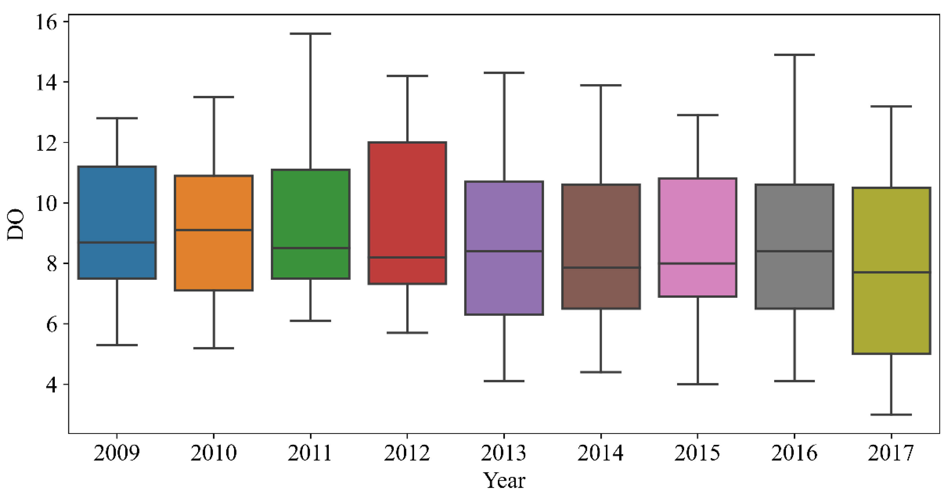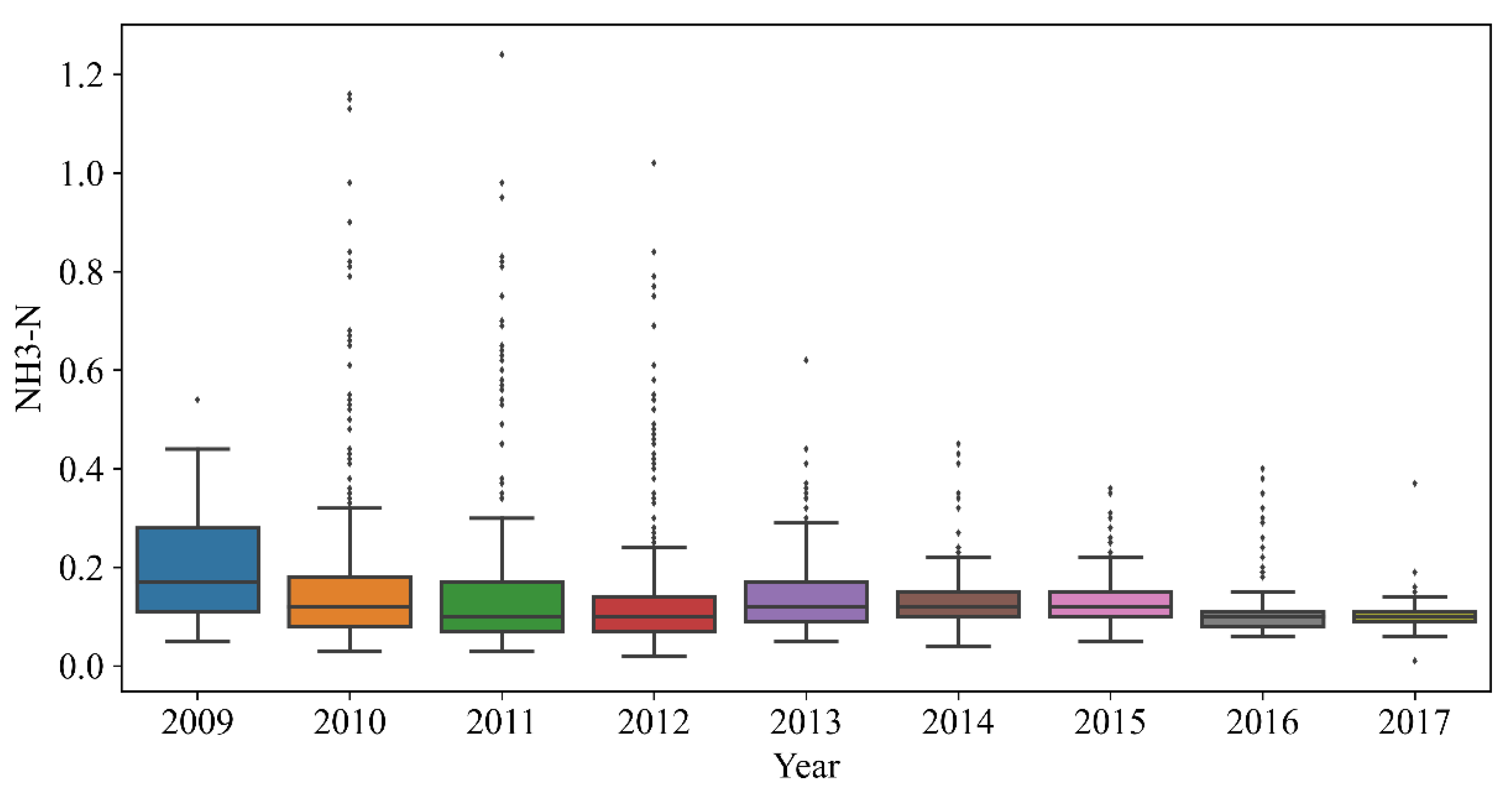The values of NH₃-N were mostly concentrated in (0, 0.2), showing a strong concentration. For the year as a unit of water quality data for the details of the division, Figure 2, Figure 3 and Figure 4 show the DO, pH, and NH₃-H in each year of the data distribution, including the average value, the highest value, and abnormal values. There was a certain regularity in the distribution of DO. The pH also gradually stabilized, and NH₃-H showed a decreasing trend year over year. Figure 5 shows the frequency distribution of the water quality level. The water quality data had five levels, and the proportion of each level was about the same. There were a certain number of abnormal values in the water quality indicator data, so we first carried out data preprocessing.

2.2. Data Preprocessing

2.2.1. Outlier Detection Method Based on Isolated Forest

In this research, we used the isolated forest algorithm [29] for outlier detection. The isolated forest (iForest) algorithm is an unsupervised anomaly detection method based on integrated learning that does not require prior knowledge of the label information of the training set. For the data space in which all samples are located, the iForest uses a random hyperplane to divide the space into two along a certain dimension, with each subspace containing only a portion of the original data, and divides the two subspaces again in the same way, repeating the above process until only one datum remains in each subspace. Because the density of the subspace where the abnormal data are located is much lower compared to the normal data clusters, the abnormal data points can be isolated with only a small number of partitions.

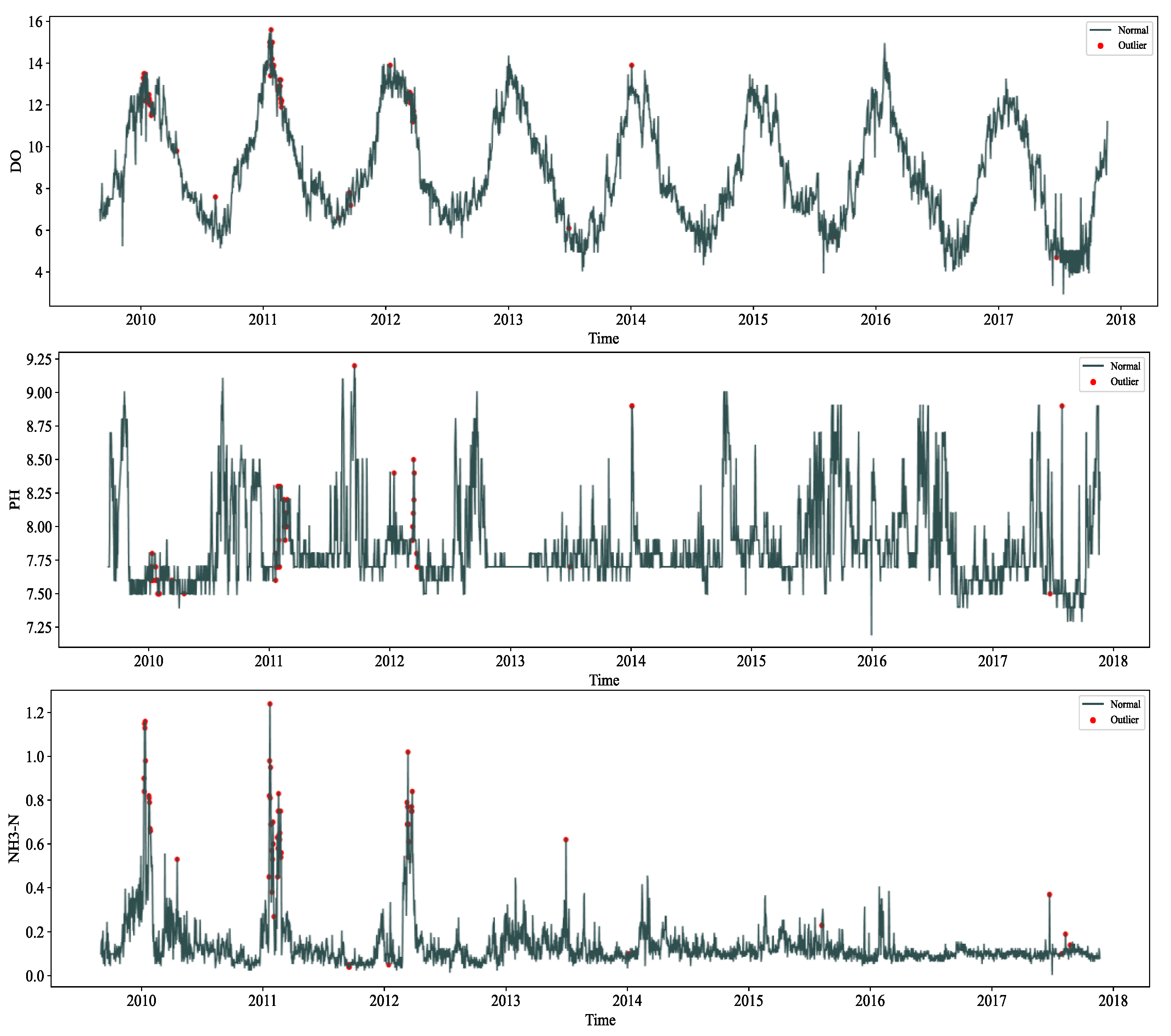
Considering the small sample data, the outlier ratio parameter setting was small; after setting the parameters, we detected the outliers on the three water quality indicator data, and the detection results are shown in Figure 6; for the detected outliers, we chose to carry out deletion and used the linear interpolation method.

2.2.2. Data Normalization

Since the dimensions of various water quality indicator data were not uniform, this study used maximum and minimum standardization to standardize the data.

$$x^{\ast }=\frac{x-min}{max-min}$$

(1)

where max is the maximum value of the data, and min is the minimum value of the data.

2.3. Correlation Analysis and Significance Test

Before conducting the correlation analysis, we conducted a normality test for each water quality indicator and found that none were consistent. Therefore, the Spearman rank correlation coefficient was used to measure the correlation between each water quality indicator.

The rank is the average descending position of the numbers in the overall data. If X and Y are two observed variables of $n$ sample sizes, for each sample ($X_i$, $Y_i$), corresponding to a rank of ($x_i$,$y_i$), the Spearman’s rank correlation coefficient $\rho$ between these two variables is

$$\rho =1-\frac{6{{\displaystyle \sum }}^{ }{d}_i^2}{n\left(n^2-1\right)}$$

(2)

where $d_i=x_i-y_i$ denotes the rank difference between the two indicators for the ith sample.

To confirm the veracity of the correlation between the two variables, a significance test of the correlation coefficient should also be performed. With a sample size of more than 30, the study constructed the statistic $r_s\sqrt{n-1}\sim N\left(0,1\right)$ and had the following hypothesis:

Original hypothesis $H_0$: the two water quality characteristics are not correlated.

Alternative hypothesis $H_1$: the two water quality characteristics are correlated.

According to the significance coefficient $p$ value, the significance test criteria were as follows:

$p$ < 0.05: there is a statistical difference; the original hypothesis is rejected, and the two water quality variables are related.

$p$ > 0.05: there is no statistical difference; the original hypothesis is accepted, and the two water quality variables are not correlated.

As can be seen from

Table 2. Results of correlation analysis of water quality indicators.

Dataset	Water Quality Indicators	NH3-N	pH	DO
All	NH3-N	1.000	−0.335	0.136
	pH	−0.335	1.000	0.006
	DO	0.136	0.006	1.000
Spring	NH3-N	1.000	−0.309	0.210
	pH	−0.309	1.000	0.121
	DO	0.210	0.121	1.000
Summer	NH3-N	1.000	−0.296	−0.044
	pH	−0.296	1.000	0.259
	DO	−0.044	0.259	1.000
Autumn	NH3-N	1.000	−0.366	−0.218
	pH	−0.366	1.000	0.099
	DO	−0.218	0.099	1.000
Winter	NH3-N	1.000	−0.221	0.211
	pH	−0.221	1.000	0.184
	DO	0.211	0.184	1.000

, for the overall data set, NH₃-N, and pH showed a weak negative correlation, DO showed a very weak positive correlation with both NH₃-N and pH, and the correlation between the water quality indicators varied with the season. In general, the correlation between the three water quality indicators was not strong.

In addition, this study chose the Spearman correlation coefficient to determine whether there was a correlation between the water quality evaluation grade and each water quality indicator. If there was no correlation, the water quality indicator should not be selected as the independent variable when evaluating the water quality level.

The correlation coefficient significance level of water quality evaluation grade and each water quality indicator was less than 0.02; hence, the original hypothesis was rejected, and it was considered a significant correlation. As can be seen from Figure 7, pH and water quality evaluation grade showed a weak positive correlation, DO and water quality evaluation grade had a moderate positive correlation, and NH₃-N and water quality evaluation grade showed a weak negative correlation.

2.4. Analysis of Seasonal Fluctuations

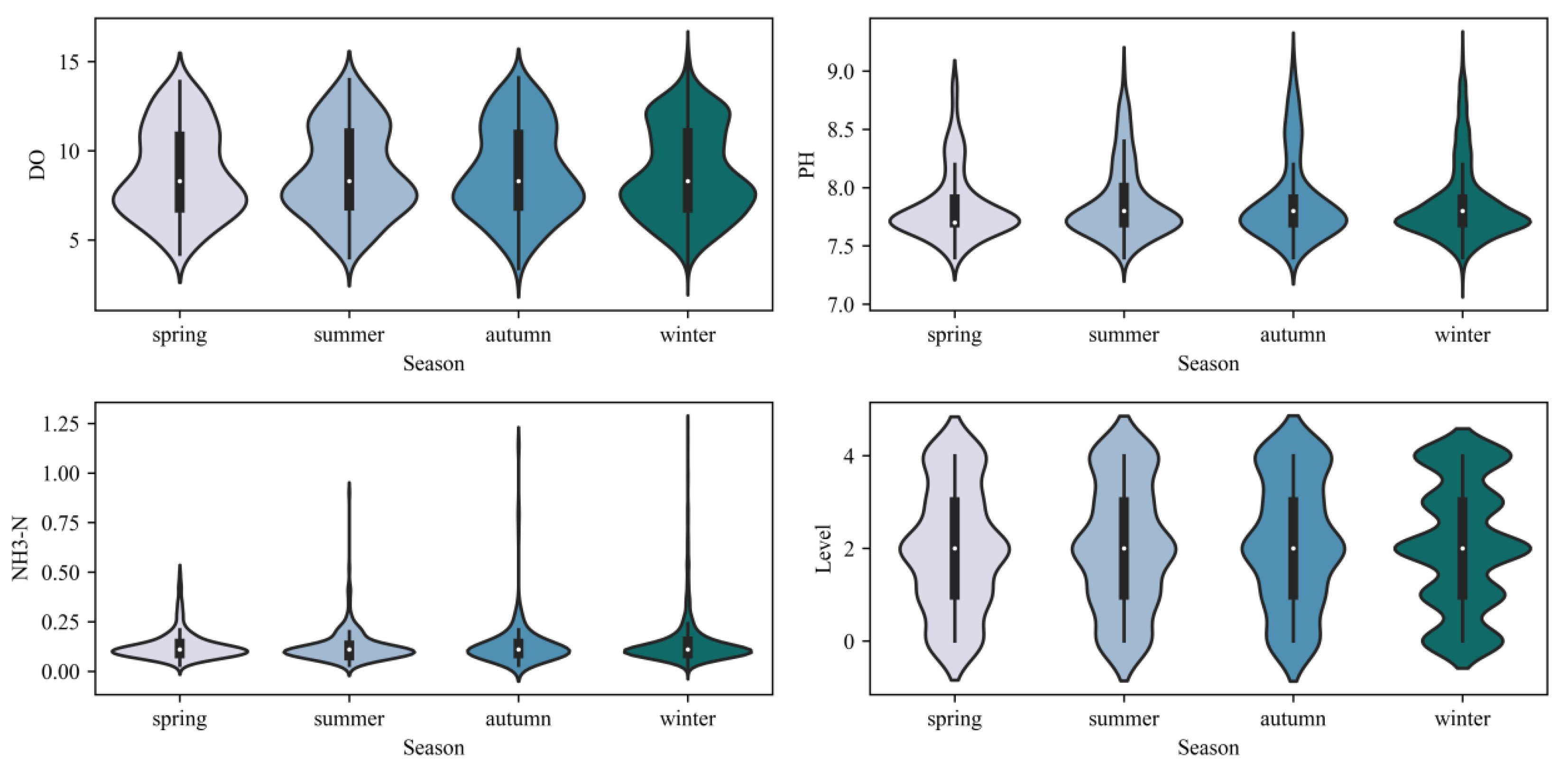
In this study, the data sets were divided by seasons, and the characteristics on the overall and four-season data sets were counted. As can be seen from Figure 8, the pH was more stable in all seasons; DO was lower in summer and higher in winter, which is consistent with the physical and chemical law that DO is lower the higher the water temperature is; NH₃-N was lower in summer and autumn and higher in winter, which is generally due to the low temperature leading to lower biochemical treatment efficiency of water flow and slower degradation of ammonia nitrogen. The mean value of water quality evaluation level in each season was approximately the same; in spring, summer, and autumn, the distribution was very similar, and in winter, there were some fluctuations in the distribution, which may be related to the low temperature.

2.5. Discrete Wavelet Transform

For water quality indicator data, this paper, from a new research perspective, attempted to decompose the original sequence data into two sequences of trend and fluctuation terms, i.e., a complex problem was broken down into two relatively well-defined sub-problems. The wavelet transform aims at multi-scale analysis of the time series signal in both the time and frequency domains [30], and it filters the original time series signal by low-pass and high-pass filters to obtain the corresponding low-frequency components and high-frequency components. The low-frequency component is the main part of the original signal and contains the overall trend of the signal, while the high-frequency component contains details or differences of the signal and often reflects short-term fluctuations of the sequence. According to the different processing data, wavelet transform can be divided into continuous wavelet transform and discrete wavelet transform. Water quality indicator data are discrete; the discrete wavelet transform representation form is as follows:

$$x_t=L_K\left(t\right)+{\displaystyle \sum }_{k=1}^K{H}_k\left(t\right)={\displaystyle \sum }_{n=1}^N{c}_{K,n}{\phi }_{K,n}\left(t\right)+{\displaystyle \sum }_{k=1}^K{\displaystyle \sum }_{n=1}^N{d}_{k,n}{\psi }_{k,n}\left(t\right)$$

(3)

where x_t is the time series data in period $t$, N is the length of the time series data, and $K$ denotes the number of discrete wavelet transforms. $L_K\left(t\right)$ denotes the low-frequency component corresponding to the K-th discrete wavelet transform in period t; H_k(t) denotes the high-frequency component corresponding to the $k-\mathrm{th}$ discrete wavelet transform in period $t$. $c_{K,n}$ and d_k,n represent the decomposition coefficients corresponding to the low-frequency component and the high-frequency component, respectively; ${\phi }_{K,n}\left(t\right)$ and ${\psi }_{k,n}\left(t\right)$ represent the low-pass filter and the high-pass filters, respectively. In general, the discrete wavelet transform can continue to decompose the low-frequency components and finally reconstruct all the high-frequency components and the low-frequency components obtained from the final decomposition into new sequence data. In the wavelet decomposition process, the more layers of decomposition, the better it is to smooth the data at each layer to capture complex information; however, if the number of decomposition layers is too many, it will lead to a larger overall prediction error. The overall error minimization principle was adopted to determine the number of wavelet decomposition layers K in the subsequent empirical analysis.

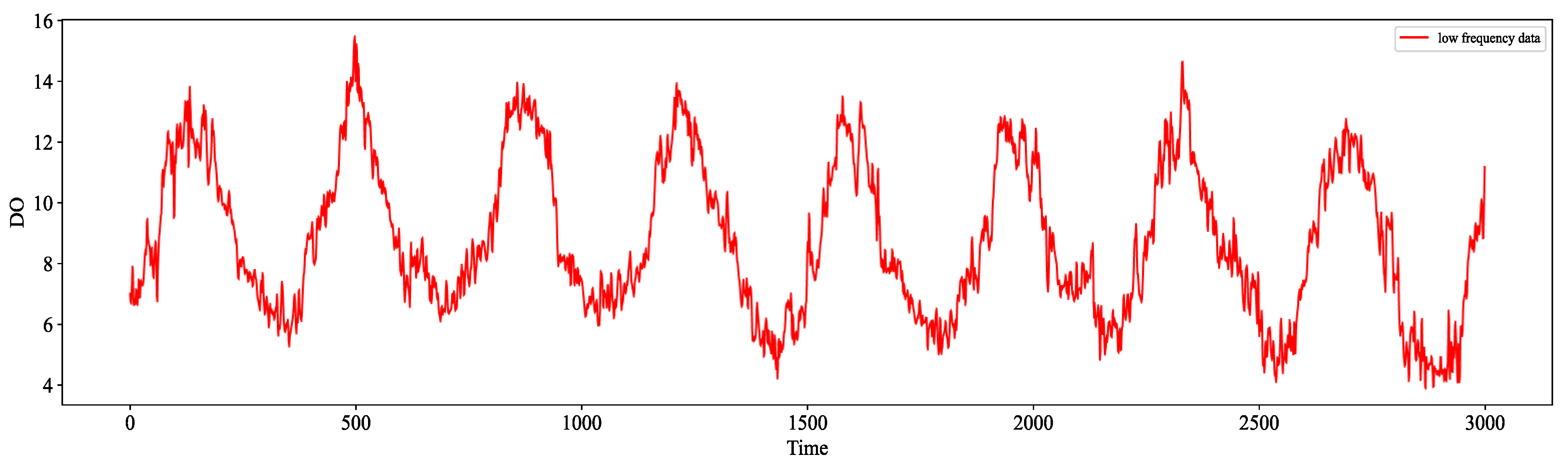
In processing time series data, haar wavelet, db wavelet, and sym wavelet are the three commonly used methods for processing wavelet decomposition. Compared with the other two wavelet bases, sym wavelet has better symmetry. So, we chose sym wavelet to decompose the data. Through wavelet transformation, we decomposed the water quality indicator data. The water quality indicator DO decomposition results are shown in Figure 9 and Figure 10, including a set of low-frequency data and a set of high-frequency data. Low-frequency data corresponded to the essential characteristics of the original data, reflecting the trend changes of the time-series data under steady-state conditions, which can well reflect the main change pattern of the data, also known as the trend term. The high-frequency data, on the other hand, mainly contained the details of the original data, reflecting the volatility and nonlinearity of the original data based on the low-frequency steady-state data, which is also called the fluctuation term.

2.6. ARIMA Model

The Autoregressive Integrated Moving Average (ARIMA) model is a very popular time series forecasting model among research scholars. It is a time series data forecasting method proposed by Box and Jenkins in 1970 [31]. It has the advantages of a simple setup and better ability to capture linear relationships. Better accuracy can be achieved by modeling the trend terms after wavelet decomposition using traditional time series forecasting methods.

The ARIMA model involves three parameters, $p$, d and $q$, where p represents the lag order of the time series data itself in the model, $d$ represents the time series data needed to be differenced to smooth data by order $d$, and $q$ represents the lag order of the prediction error in the model. The ARIMA model contains three special types, including an autoregressive model (AR), a moving average model (MA), and an autoregressive moving average model (ARMA). The AR ($p$) model predicts the current value based on historical value information, as shown in Equation (4). $y_t$ is the current value, $\mu$ is the constant term, ${\alpha }_i$ is the autocorrelation coefficient, and ${\epsilon }_t$ is the difference term. The MA (q) model predicts the current value based on the accumulation of historical error terms, as shown in Equation (5), and the ARMA ($p$,$q$) model is a combination of the AR ($p$) and MA ($q$) models, as shown in Equation (6).

$$y_t=\mu +{\displaystyle \sum }_{i=1}^p{\alpha }_i{y}_{t-1}+{\epsilon }_t$$

(4)

$$y_t=\mu +{\displaystyle \sum }_{i=1}^q{\beta }_i{\epsilon }_{t-1}+{\epsilon }_t$$

(5)

$$y_t=\mu +{\displaystyle \sum }_{i=1}^q{\beta }_i{\epsilon }_{t-1}+{\epsilon }_t+{\displaystyle \sum }_{i=1}^p{\alpha }_i{y}_{t-1}+{\epsilon }_t$$

(6)

The data input to the ARIMA model in this study were the trend terms after wavelet decomposition, and after the first and second differencing, the effect was indistinguishable from no differencing, so $d=0$. Secondly, BIC was used to determine the $p$ and $q$ parameters of ARIMA. In this study, we calculated the BIC value under $p$, $q$ ∈{0, 1, …, 9}, and $p$, q were automatically selected by the correlation function for the case of the minimum BIC index.

2.7. Gated Recurrent Unit (GRU) Model

After fitting the trend term using the ARIMA model, the GRU model [32] was introduced to explain the fluctuation term and fuse the final prediction results to improve the prediction accuracy for nonlinear and nonstationary small sample data. The internal structure of the GRU model is shown in Figure 11.

A GRU contains two gate functions, i.e., an update gate and reset gate. Among them, $x_t$ is the input data at time $t$, h_t is the output data or hidden layer unit output at time $t$, C means two vector connected operations, X means multiplying the two parts of input data, and 1- means subtracting the data input to the module by 1. u_t means the update gate, whose main function is to control the degree of state information from the previous moment into the current state, and a larger value means that the current moment incorporates more state information than the previous state. $r_t$ is the reset gate, whose main function is to control the proportion of information from the previous state to the current state hidden cell candidate $\widetilde{h_t}$. $\sigma$ is the $sigmoid$ activation function, whose output range is (0, 1), and $tanh$ is the hyperbolic tangent activation function, whose output range is (−1, 1).

Information entering the GRU unit is passed in the following flow.

• The input data at moment $t$ and the hidden layer output at moment $t-1$ are spliced to obtain the reset gate output signal r_t using Equation (7).
• The update gate output signal $u_t$ is obtained using Equation (8).
• The current set of hidden cell candidates $\widetilde{h_t}$ is obtained using Equation (9), which mainly combines the input data and the state of the hidden layer at moment $t-1$ after the reset gate screening.
• The hidden layer output at moment $t$ is obtained using Equation (10), which indicates forgetting the hidden layer information $h_{t-1}$ delivered at moment $t-1$ and filtering the important information output in the candidate hidden layer at moment $t$. $\left(1-u_t\right)\ast h_{t-1}$ denotes selective forgetting of the hidden state at the moment $t-1$, $u_t\ast \widetilde{h_t}$ denotes selective forgetting of the candidate set of hidden units $\widetilde{h_t}$, and only the important information in $\widetilde{h_t}$ is retained. This cycle is repeated to achieve the accumulation of historical information and memory, which can effectively capture the long-range correlation existing in water quality prediction or a time series model.

$$r_t=\sigma \left(W_r\cdot \left[h_{t-1},x_t\right]\right)$$

(7)

$$u_t=\sigma \left(W_u\cdot \left[h_{t-1},x_t\right]\right)$$

(8)

$$\widetilde{h_t}=tanh(W_{\tilde{h}}\cdot \left[r_t\ast h_{t-1},x_t\right])$$

(9)

$$h_t=\left(1-u_t\right)\ast h_{t-1}+u_t\ast \widetilde{h_t}$$

(10)

2.8. LightGBM

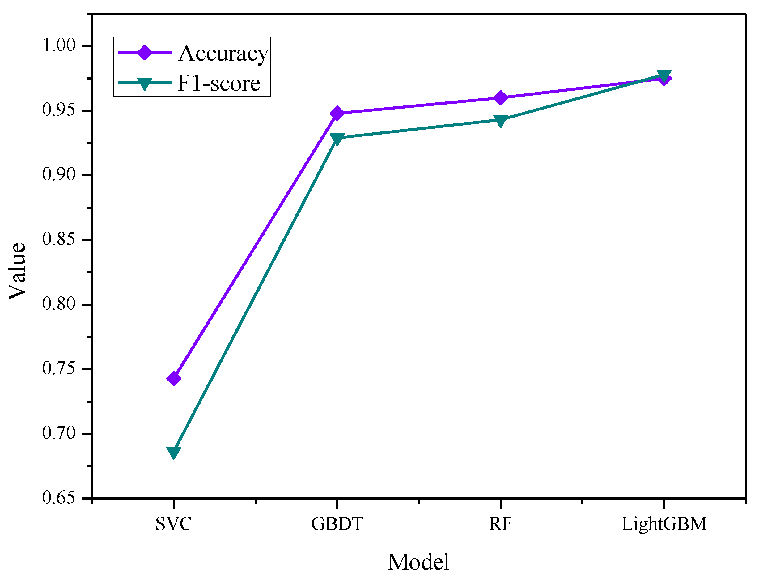
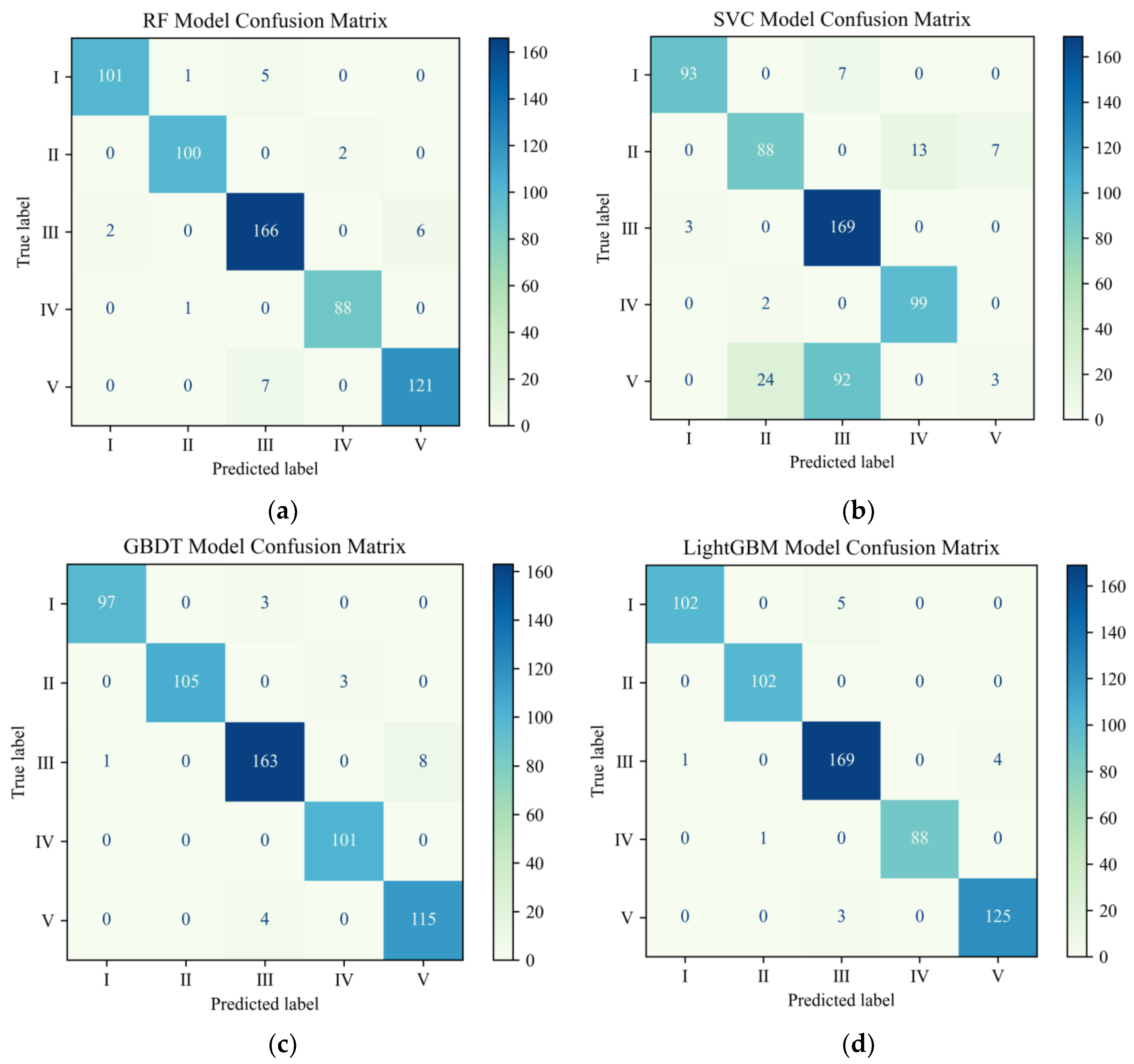
LightGBM is an augmented integrated tree algorithm (Boosting) [33], which derives multiple decision trees successively from one decision tree by continuous augmentation, and each decision tree computes the gradient descent direction of its own loss function to generate a new decision tree. The algorithms that belong to this category of Boosting also include GBDT, AdaBoost, XGBoost, etc. These Boosting methods in the current machine learning field have the most powerful performance, but in the field of water quality prediction, they have not been widely used. This paper used the algorithm for water quality evaluation level prediction, research also based on Support Vector Machine (SVM), Random Forest (RF), and Gradient Boosting Decision Tree (GBDT), to build a water quality evaluation level prediction model, along with LightGBM-built prediction. The models are compared with LightGBM in terms of different methods and different learning strategies. Among them, SVM and other models can form a comparison between a non-tree model and a tree model, RF and LightGBM form a comparison between integrated Bagging strategy and Boosting strategy, and GBDT and LightGBM form a comparison of similar Boosting methods.

2.9. Integrated Time Series Model

For the time-series prediction of water quality indicator data, different time-series prediction models were used to analyze the low-frequency data and high-frequency data according to the characteristics of discrete wavelet transform decomposition. Specifically, for low-frequency data, this paper used the ARIMA time series prediction model; the model in the data under the steady-state and linear conditions can more accurately reflect the dynamic changes in the data and result in a high prediction accuracy. In addition, this method has the advantages of fast training speed and less overfitting compared with deep learning prediction methods. The GRU deep prediction model was used to predict the dynamics of decomposed high-frequency data for the characteristics of severe nonlinearity and strong volatility. GRU can effectively capture the long and short time series information through the introduction of the gate structure, so as to obtain more accurate time series prediction results. The combined water quality indicator prediction model (W-ARIMA-GRU) proposed in this paper is shown in Figure 12. Through wavelet decomposition to obtain the trend term and fluctuation term sets of data, respectively using the ARIMA model and GRU model for prediction, the corresponding sum of the predicted values obtained is the final prediction value of the model.

2.10. Model Evaluation Methods

2.10.1. Water Quality Indicator Model Evaluation

In this paper, we choose three evaluation indexes as the basis for judging the prediction effect of the water quality indicator model: Root Mean Squared Error (RMSE), Mean Absolute Error (MAE), and the R-squared value.

The MAE is used to describe the difference between the predicted value and the true value. The smaller the value, the better.

$$\mathrm{MAE}=\frac{1}{n}{\displaystyle \sum }_{i=1}^n\left|f_i-y_i\right|$$

(11)

The RMSE is very sensitive to the error in the size of the prediction results in the training set, so it can be a good indicator of the prediction accuracy. The smaller the value, the better.

$$\mathrm{RMSE}=\sqrt{\frac{1}{n}{\displaystyle \sum }_{i=1}^n{\left(f_i-y_i\right)}^2}$$

(12)

The R2 score, also known as the Coefficient of Determination, determines how well the predicted value fits the true observed value. The best value (upper limit) is 1, or it can be negative. The closer to 1, the better.

$$R^2=1-\frac{{{\displaystyle \sum }}_{i=1}^n{\left(y_i-f_i\right)}^2}{{{\displaystyle \sum }}_{i=1}^n{\left(y_i-\stackrel{-}{y}\right)}^2}$$

(13)

2.10.2. Water Quality Level Model Evaluation

For the water quality class multi-classification problem, multiple evaluation metrics are needed. In this paper, three evaluation metrics—accuracy, F1-score, and confusion matrix—were used. The confusion matrix is shown in

Table 3. Confusion matrix.

	True Label	Positive	Negative
Predicted Label
Positive		True Positive (TP)	False Positive (FP)
Negative		False Negative (FN)	True Negative (TN)

. Each row of the confusion matrix indicates the true category of the data. The number of all data instances in each row indicates the number of instances in this category. Each column represents the prediction category, and the total number of each column represents the number of predictions for this category. The accuracy is the proportion of the number of correctly classified samples to the total number of samples in the given data, as shown in Equation (14). The F1-score is the summed average of accuracy and recall, as shown in Equation (17) [34,35].

$$Accuracy=\frac{TP+TN}{TP+TN+FN+FP}$$

(14)

$$Precision=\frac{TP}{TP+FP}$$

(15)

$$Recall=\frac{TP}{TP+FN}$$

(16)

$$F_1=\frac{2\times precision\times recall}{precision+recall}$$

(17)

3. Results

3.1. Water Quality Indicator Prediction Model Validation and Analysis

In order to verify the validity of the proposed model, we used surface water quality data collected and compiled by Zhongguancun International Medical Inspection and Certification Co., Ltd., from 2009 to 2017 in a region of Beijing to validate the water quality index prediction model. We used three time series data—DO, pH, and NH₃-N—for validation and used the ablation experiment method to compare the model effect. The parameters of the GRU model following parameter tuning are shown in

Table 4. Parameters setting of GRU model.

Parameter	Value
Time Steps (s)	30
Input Layer Unit Number	100
Output Layer Unit Number	1
Hide Layer Number	2
Hide Layer Unit Number	100
Epochs	30
Batch Size	32
Activation Function	Rectified linear unit (ReLU)
Loss Function	Mean absolute error (MAE)
Optimizer	Adam
Learning Rate	0.001

.

First, we studied the prediction of water quality indicator data considering a time step of 30 (one month) using the combined W-ARIMA-GRU model, and the effect of the prediction curve is shown in Figure 13.

Using MAE, RMSE, and R2 values as evaluation metrics, the prediction of each model on this data set using the ablation experimental approach is shown in

Table 5. Prediction results of each model.

Experimental Subjects		Evaluation	MAE	R2	RMSE
	Model
DO	SVR		0.8578	0.8306	1.0369
	TCN		0.4891	0.9356	0.6389
	LSTM		0.4508	0.9433	0.5997
	ARIMA		0.4333	0.9465	0.5828
	GRU		0.4448	0.9421	0.5838
	W-LSTM		0.3476	0.9631	0.4743
	W-GRU		0.2479	0.9813	0.3411
	W-ARIMA-LSTM		0.2776	0.9773	0.3746
	W-ARIMA-GRU		0.2395	0.9828	0.3275
pH	SVR		0.1716	0.5857	0.2465
	TCN		0.1404	0.7051	0.2080
	LSTM		0.1322	0.7241	0.1980
	ARIMA		0.1339	0.7214	0.2021
	GRU		0.0985	0.7912	0.1527
	W-LSTM		0.0812	0.8835	0.1189
	W-GRU		0.0801	0.8956	0.1172
	W-ARIMA-LSTM		0.0902	0.8750	0.1229
	W-ARIMA-GRU		0.0734	0.9213	0.1068
NH3-N	SVR		0.0071	0.6418	0.0105
	TCN		0.0070	0.6689	0.0099
	LSTM		0.0068	0.7035	0.0087
	ARIMA		0.0070	0.6786	0.0098
	GRU		0.0068	0.7085	0.0085
	W-LSTM		0.0064	0.7254	0.0081
	W-GRU		0.0062	0.7456	0.0078
	W-ARIMA-LSTM		0.0055	0.8456	0.0068
	W-ARIMA-GRU		0.0054	0.8513	0.0065

. The R2 values of the proposed model were 0.9828, 0.9213, and 0.8513 for the three studied subjects, respectively, which were higher than the other models. The MAE and RMSE were also minimized accordingly. With a time-step of 30, eight comparison models were included: SVR, Temporal Convolutional Network (TCN), LSTM, ARIMA, GRU, Wavelet-LSTM (W-LSTM), Wavelet-GRU (W-GRU), and Wavelet-ARIMA-LSTM (W-ARIMA-LSTM). The proposed model exhibited good results.

Next, we took the input time step as the independent variable and studied the effect of the proposed model at different time steps. Taking the water quality indicator DO as an example, the specific evaluation results are shown in Figure 14, in which 13 rounds of experiments were conducted, corresponding to time steps of 1, 3, 7, 10, 15, 20, 30, 45, 60, 90, 120, and 180.

From the comparison graph of the prediction effects, it can be seen that the R2, MAE, and RMSE values of single deep learning models such as LSTM and GRU models fluctuated more as the time step increased, and the prediction effects of the LSTM and GRU models showed a decreasing trend when the time step exceeded 90 [36]. After adding wavelet decomposition, the variation of the R2, MAE, and RMSE values of the LSTM and GRU models became smaller, the prediction stability improved substantially, and the prediction effect improved, which also proved that the effect of adding wavelet decomposition would improve nonstationary time-series data. Finally, when the ARIMA model was used to predict the decomposed trend terms instead of the LSTM and GRU models, the R2 value was greatly improved compared with the previous models, and the MAE and RMSE values were significantly reduced, with the R2 value of the W-ARIMA-GRU model exceeding 0.98 at different time steps, while the MAE and RMSE were below 0.3 and 0.4, respectively, showing the model’s great advantages.

3.2. Water Quality Level Prediction Model Validation and Analysis

We used the LightGBM model for water quality level prediction, and after a grid search, the main parameters of the model were set as shown in

Table 6. LightGBM parameter tuning table.

Parameter	Value
n_estimators	20
max_depth	−1
num_leaves	31
max_bin	125
lambda_l1	0.05
lambda_l2	0.5
min_split_gain	0
learning_rate	0.1
sub_sample	0.8
bagging_freq	5
min_data_in_leaf	80

.

With DO, NH₃-N, and pH as input variables and water quality evaluation grade as the dependent variable, experiments were conducted on the SVC, GBDT, RF, and LightGBM models; the evaluation results of each model are shown in Figure 15. The confusion matrix of each model is shown in Figure 16.

From the water quality evaluation grade prediction effect comparison chart, it can be seen that the traditional machine learning prediction model SVC had the lowest prediction effect; the accuracy and F1-score were only 74.3% and 68.9%, and the effect was more general. Compared with the SVC model, the prediction effect of the tree model was greatly improved; the LightGBM model accuracy and F1-score reached 97.5% and 97.8%, respectively, ahead of the other integrated learning models, which once again verified the powerful performance of the LightGBM model. This paper used the model for the prediction of water quality evaluation grade and achieved very good results.

4. Discussion

Water is the source of life. In recent years, water pollution events have emerged one after another. Water quality prediction is a major research hotspot. The evolution and development of water quality is affected by many variables, such as the influence and interference of physics, chemistry, biology, meteorology, and hydraulics. Fixed mathematical expressions make it difficult to solve strong nonlinear characteristics. In addition, traditional time series models have poor generalization performance for time series data tables with high volatility. The W-ARIMA-GRU water quality indicator prediction model proposed in this paper has good applicability and robustness for the analysis and prediction of nonlinear problems in uncertain environments. The model can be used to monitor the real time change trend of water quality data and to judge and warn of possible risks. When the water quality situation deteriorates, relevant management departments can make decisions as soon as possible and formulate effective prevention and control measures in time to effectively avoid potential water pollution incidents.

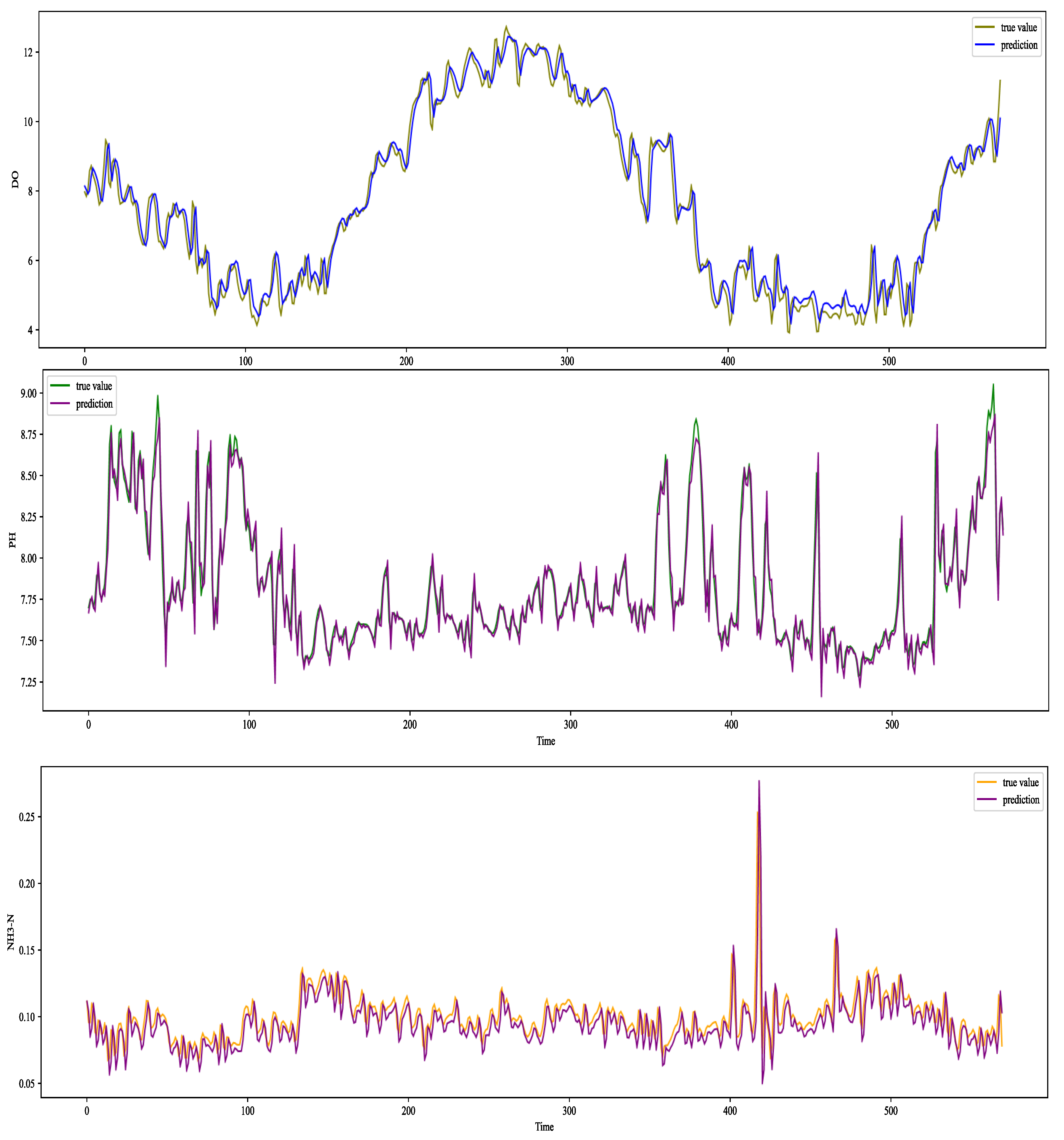
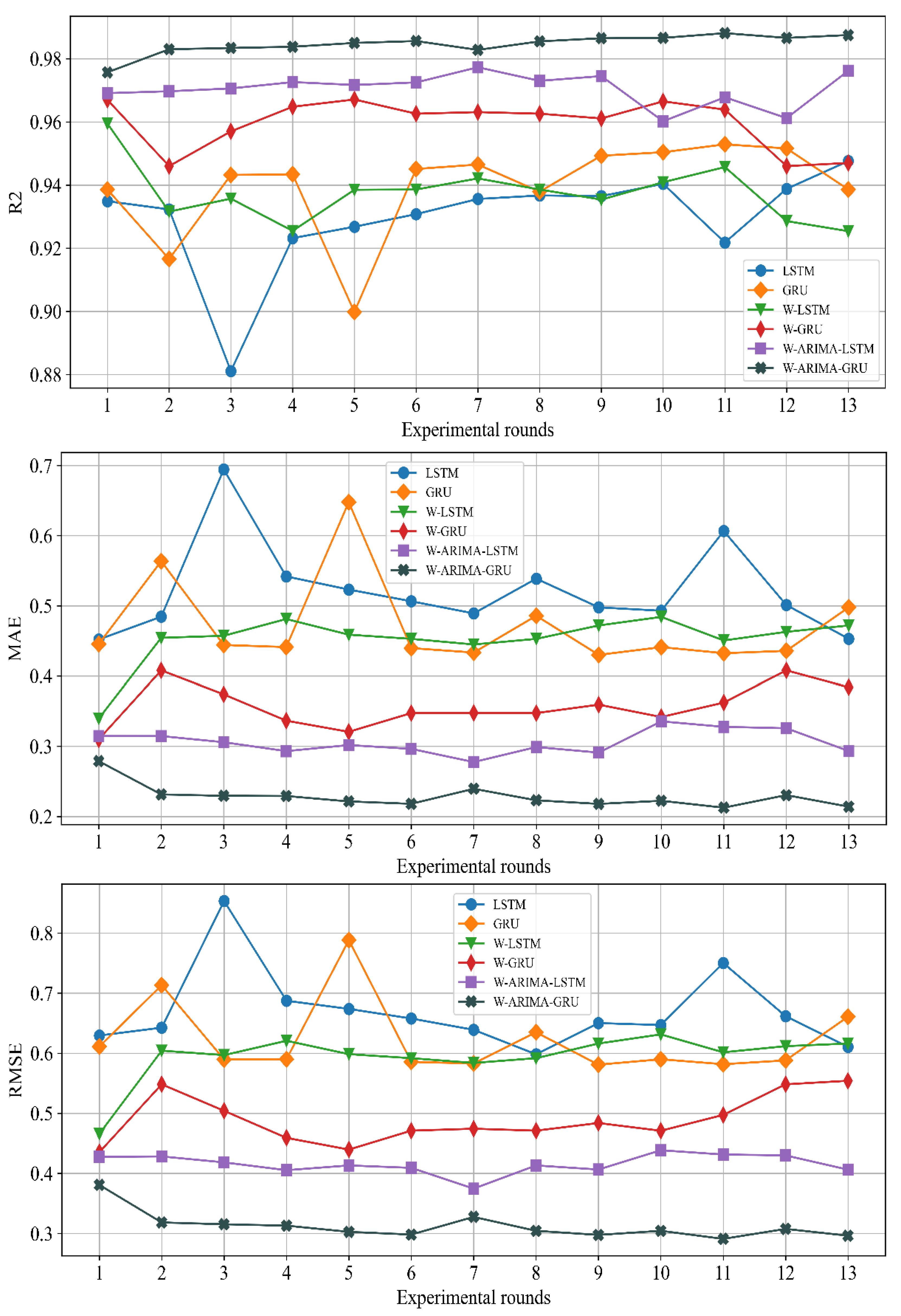
Different from the existing popular ensemble learning strategies mainly based on the Bagging method [37] and the Boosting method [38], from a new research perspective, this paper decomposed the original sequence data into two sequences of trend items and fluctuation items, namely, one complex problem was broken down into two relatively clearly defined sub-problems. According to the characteristics of the decomposed sequence data, the traditional time series prediction method was used to model the trend item, the deep learning method was introduced to explain the fluctuation item, and the final prediction results were fused to improve the analysis of nonlinear and nonstationary small items. In terms of the prediction accuracy of the sample data, the experiments showed that when the research object was the water quality indicator DO, the MAE and RMSE of this model were at least 0.114 and 0.136 lower than the other models. The R2 improved by at least 0.0015. When the research object was the water quality indicator pH, the MAE and RMSE of this model were at least 0.0065 and 0.0094 lower than the other models. The R2 improved by at least 0.0357. When the research object was the water quality indicator NH₃-N, the MAE and RMSE of this model were at least 0.0001 and 0.0003 lower than the other models. The R2 improved by at least 0.0057. When changing the time step, taking the water quality indicator DO as the research object, the R2 value of the W-ARIMA-GRU model exceeded 0.98 at different time steps, while the MAE and RMSE were below 0.3 and 0.4, respectively, showing the model’s great advantages. In addition, we introduced the LightGBM model into the prediction of water quality evaluation grades and found that the accuracy and F1-score of the LightGBM model reached 97.5% and 97.8%, respectively, which were higher than other models by at least 0.012 and 0.0178. Thus, we established an efficient prediction framework that can be used for water quality indicators and water quality evaluation levels.

There are still several areas for improvement in this study.

(1)

The model proposed in this paper showed a good effect on short-term water quality prediction, but when we tried to predict long-term effects, the prediction was not satisfactory. In future, we will try to combine other models to improve their long-term prediction performance.

(2)

In this study, we used a two-layer GRU model; we will attempt to build a mixture of the LSTM model and the GRU model in the future and compare it with other models.

(3)

Due to the conditions, we only extracted the temporal features of a fixed area. If there are data in other areas, we could consider using the graph neural network [39] to extract spatial features, so as to reflect the overall spatial change of water quality; thus, a more complete water pollution early warning system can be established.

(4)

We used fewer data on water quality indicators in water quality level prediction; using more water quality indicator data to predict water quality evaluation grades would provide more robust results.

5. Conclusions

This paper used surface water quality data collected and compiled by Zhongguan-cun International Medical Inspection and Certification Co., Ltd. (Beijing, China), from 2009 to 2017 in a region of Beijing as the research object and aimed to establish a proven water quality prediction framework. We first used the W-ARIMA-GRU model to predict three conventional water quality indicators, DO, pH and NH₃-N, and the model had good performance as well as strong robustness. Next, we used the three water quality indicators for water quality grade prediction, without considering other water quality indicators; the accuracy and F1-score of the LightGBM model for water quality grade prediction reached 97.5% and 97.8%, respectively. We believed that we have established a prediction framework for water quality indicators and level. The sampling site was located in the suburbs for the detection of water quality using discrete sampling. The analysis process was more complicated, and there was a significant resource depletion problem. The model can be used for local monitoring of real-time trends in water quality data. In addition, the use of three conventional water quality indicators for water quality level classification was useful, as this small number of conventional water quality indicators could increase online water quality level prediction, thus greatly reducing the offline workload and unnecessary use of resources. At the same time, our proposed W-ARIMA-GRU water quality indicator prediction model had good universality and high efficiency; it could also be used for other rivers, lakes, and reservoirs and to judge and warn of possible water quality pollution risk when there is a trend of deteriorating water quality conditions. The relevant management departments can make early decisions and develop effective prevention and control measures, so as to effectively avoid potential water pollution events.

In this paper, through the study of water quality time series data, we predicted the possible future situation of water quality in a region of Beijing. We only extracted the temporal characteristics of a fixed region; for other regions of water quality data, in the future, we will consider the topological relationship between the regions and will use graphical neural networks for spatial feature extraction, so as to reflect the spatial and temporal changes in water quality. This will allow establishment of a more complete water pollution early warning framework for timely water quality prediction and provide theoretical models and scientific reference for the relevant departments to address potential issues.