Article

A Hybrid Data-Driven-Agent-Based Modelling Framework for Water Distribution Systems Contamination Response during COVID-19

1
Faculty of Civil and Environmental Engineering, Technion-Israel Institute of Technology, Haifa 32000, Israel
2
Civil and Architectural Engineering and Mechanics, University of Arizona, Tucson, AZ 85721, USA
3
Department of Civil, Construction, and Environmental Engineering, North Carolina State University, Raleigh, NC 27695, USA
*
Author to whom correspondence should be addressed.
Water 2022, 14(7), 1088; https://doi.org/10.3390/w14071088
Submission received: 3 March 2022 / Revised: 25 March 2022 / Accepted: 28 March 2022 / Published: 29 March 2022
(This article belongs to the Section Urban Water Management)

Abstract

:
Contamination events in water distribution systems (WDSs) are highly dangerous events in very vulnerable infrastructure where a quick response by water utility managers is indispensable. Various studies have explored methods to respond to water events and a variety of models have been developed to simulate the consequences and the reactions of all stakeholders involved. This study proposes a novel contamination response and recovery methodology using machine learning and knowledge of the topology and hydraulics of a water network inside of an agent-based model (ABM). An artificial neural network (ANN) is trained to predict the possible source of the contamination in the network, and the knowledge of the WDS and the possible flow directions throughout a demand pattern is utilized to verify that prediction. The utility manager agent can place mobile sensor equipment to trace the contamination spread after identifying the source to identify endangered and safe places in the water network and communicate that information to the consumer agents through water advisories. The contamination status of the network is continuously updated, and the consumers reaction and decision making are determined by a fuzzy logic system considering their social background, recent stress factors based on findings throughout the COVID-19 pandemic and their location in the network. The results indicate that the ANN-based support tool, paired with knowledge of the network, provides a promising support tool for utility managers to identify the source of a possible water event. The optimization of the ANN and the methodology led to accuracies up to 80%, depending on the number of sensors and the prediction types. Furthermore, the specified water advisories according to the mobile sensor placement provide the consumer agents with information on the contamination spread and urges them to seek for help or support less.

1. Introduction

Water distribution systems (WDSs) are crucial infrastructure to ensure the delivery of potable drinking water to consumers and are highly critical for public health. As this infrastructure is highly vulnerable, WDSs need to be monitored as much as possible. While the drinking water can be easily monitored at the source after treatment, monitoring all relevant water quality parameters in the entirety of a water network is not feasible. In case of a water quality anomaly or even if contamination occurs, the event might go undetected, and consumption of the water could cause harm to consumers. For monitoring important water quality parameters such as pH, residual chlorine, conductivity, and turbidity at strategically crucial points in the water network, fixed water quality sensors have proven to be efficient [1,2]. For the efficient, economical utilization of these sensors, optimization methods and algorithms have been developed for determining their number and the locations to place them. By using these fixed water quality sensors, anomalies and deterioration in water quality can be detected efficiently and consumers can be warned upon the detection of a water event. Among these optimization algorithms are genetic algorithms, which are a very efficient support tool for early warning systems that detect anomalies in a drinking water network [3,4]. Inline mobile sensors, which sample water flowing inside the water network and transmit these data [5], have proved to be rather ineffective compared with conventional sensors considering the performance per cost [6,7]. However, recent studies [8,9] have shown the efficiency of placing mobile sensor equipment for collecting information on the contamination plume and to inform the consumers about the event in real time.
Furthermore, studies have used machine learning methodologies to detect water quality anomalies and their sources by training these algorithms with specific water quality parameters as input features to predict possible water events. Artificial and convolutional neural networks (ANN/CNN) and support vector machines (SVM) have been used to detect whether a contamination event has occurred in a water network [10,11]. While standardized methods to identify contamination sources involve metaheuristic optimization methods such as genetic algorithms [12,13], there have been recent implementations of machine learning to predict the contamination source of water systems. While ref. [14] were already using ANNs to reversely interpret transport patterns to track the source of Escherichia coli bacteria in a water system, Ref. [15] used concentration levels of a sensor network in a river system as input features for a random forest model to identify the source location of a specific contaminant. Moreover, an approach to utilize the random forest algorithm to identify the source of a contamination in a WDS has been presented in [16]. Various contamination events in two different water network systems were investigated and the sensor readings of a variety of sensor layouts were taken as the dataset to train the random forest model. The study presented the accuracy of the suggested framework to determine the possible source nodes.
Agent-based modelling (ABM) is a highly suitable tool to simulate complex adaptive systems (CASs) [17]. ABMs assess the situation of autonomously decision making entities (agents) which interact by specific rules, formulas and relationships and can display unexpected emergent phenomena [18]. Sophisticated models can incorporate learning methodologies of agents such as evolutionary programming or supervised machine learning models. Agent-based modelling frameworks have been used in water resources management for applications such as the estimation of residential water demand by developing a model for the evaluation of water pricing policies, or simulating the consumer behaviour of individual households [19,20]. ABM has been used to simulate water resource allocation of the Nile river, where the optimization of the water distribution was achieved by using evolutionary algorithms [21]. Furthermore, Ref. [22] used ABM to assess the risks of management strategies of water utilities for their water supply systems, where all the involved stakeholders such as the consumers, policy makers, water supply companies and the infrastructure itself were all part of the modelling framework and in-situ data were used to validate the model.
Agent-based frameworks have also been used for modelling the relationships between the WDS, the consumers and utility manager during a contamination event in a WDS [17,23,24,25]. ABMs represent and explore dependencies and feedbacks of the stakeholders during a contamination event—stakeholders such as policy makers, health officials, and consumers, among others—in a way that cannot be expected and achieved with traditional modelling. Ref. [23] used an ABM framework with an integrated evolutionary algorithm to determine an optimal flushing strategy in case of a contamination and developed new approaches for threat management by flushing specific sets of hydrants upon the event detection. The general objective here is to maximize the number of consumers that can be protected from ingesting contaminated drinking water. This model was expanded in [17] to model the mobility of consumer agents between residential nodes of the water network. These socio-technological modelling approaches, that couple an ABM with a hydraulic simulation framework, can be used to exhibit the dynamics of a water event by modelling the actions and reactions of the consumers and the utility manager agent and the consequences of their subsequent decisions [26,27]. There are various methods to model decisions or compliances with water advisories e.g., with statistical models or the evaluation of survey data [17,23]. Nevertheless, even using survey data, modelling human behaviour is very complex as humans are not simply rational decision-making beings and their emotional and psychological processes need to be taken into consideration [27].
With the global COVID-19 pandemic, which broke out in December 2019 and led to a worldwide health crisis, the reactions of the population on a behavioural level can be explored and the effects of a disaster situation on the psychological states of individuals of different societal backgrounds has been explored in recent studies [28,29,30]. The authors of [30] have conducted a large behavioural study on science communication and leadership for responding successfully to the COVID-19 pandemic, while the authors of [31] have studied the implications of the shutdowns on the water infrastructure. Furthermore, Ref. [32] developed numerical and agent-based models to simulate COVID-19 outbreaks, their dynamics and the interactions of various population agents while Ref. [33] created an ABM framework to explore the economic and health effects of the pandemic related shutdowns and restrictions. The COVID-19 pandemic also has a direct influence on the water quality. As the usage of disposable plastic face masks for protection against infection with COVID-19 has rapidly increased, the influence on the environment of the disposal of these masks, which carry traces of heavy metals, was investigated in [34,35]. Considering the enormous amount of masks that are being used and disposed of every day, major water contaminations may occur in the future. Ref. [36] used machine learning to determine the morbidity of COVID-19 patients by sampling their blood and utilizing matrix factorization methods and random forest algorithms. Furthermore, the studies of [37,38] used neural networks and a Naïve Bayesian classifier to classify blood samples to predict the severity of the COVID disease in patients.
This study develops an approach to the response to, and recovery from, any contamination event in a WDS during a global pandemic. This approach uses a model that has been developed in a recent study to connect the findings from social and behavioural data with an ABM framework that is coupled to a hydraulic model. A deep learning model is trained to identify the source of the contamination and the utility manager agent is responsible for placing the mobile sensor equipment to retrace the fate of the contamination plume and to eventually warn the water consumers that are in danger of possibly ingesting contaminated, non-potable water. Information on the water quality can be determined by dividing the water network into safe and non-safe divisions of the water network. The reaction of the consumer agents to the pandemic and the water contamination event is modelled according to recent findings in social and behavioural sciences, and the use of artificial intelligence methodologies for the response of the utility manager agent make the overarching goal of this study to develop a comprehensive socio-technological respond-and-recovery model for a water event in a water network. The motivation of this study is to use timely and innovative artificial intelligence approaches to handle and utilize a large amount of data to develop a real-time support tool for responding to a contamination event. Moreover, this work can be used as a proof of concept for constructing a framework which can be utilized for any kind of water network and scenario as it incorporates reactions, interactions and interdependencies among consumers, utility managers, environmental stress, network topology, hydraulics and water quality data.
The rest of this study includes a description of the developed modelling framework, an example application, the work’s conclusions, and future work.

2. Modelling Framework

An agent-based modelling framework is built to explore a deep learning response-and-recovery methodology for a contamination event in a WDS during a pandemic, and to observe the consumer agent’s behaviour in response to both threats.

2.1. ABM Framework Coupled to a Hydraulic Simulator

According to [39], an ABM simulator has to incorporate the following five steps: (1) initialisation of the parameters, environment and the initial state of the agents; (2) a time loop for processing each timestep; (3) an agent loop to route the agents; (4) updating each agent behaviour at each timestep; and (5) saving the data for further analysis. This was hardcoded from scratch into a MATLAB (v. 2020, from the MathWorks Inc., sourced with a student license from the Israel institute of Technology, Haifa, Israel) based agent-based model where every entity and parameter were programmed by the authors of this study. The details of the ABM model and all key parameters are explained in [9]. As this study is based on the aforementioned ABM framework, the most important functionalities and basic data will be described. The coupling of the hydraulic and the ABM can be achieved through MATLAB as the hydraulic and water quality simulations are conducted with an EPANET-MATLAB toolkit [40], which uses EPANET 2.0 [41] as the hydraulic simulator and the multispecies extension of EPANET (EPANET-MSX) [42] as the water quality simulator. As the ABM is programmed in MATLAB, the hydraulic simulator can be embedded into the framework’s loop and all hydraulic parameters and variables are continuously accessible so that the demands and hydraulics can be adjusted according to the current behaviour of the agents as shown in Figure 1. The figure shows the conceptual flowchart of the simulation dependencies. The water distribution system, represented by the hydraulic simulator, delivers water quality information to the utility manager and the possibility that contaminated drinking water could be delivered to the consumers. The support tool of the utility manager agent, which includes an artificial neural network (ANN), identifies the source of the contamination that determines where the utility manager will place the mobile sensor equipment. Furthermore, the utility manager sends out a water advisory through various media channels to warn the water consumers about the water event. While the placement of the mobile sensor equipment helps to divide the water network into safe and non-safe partitions, the water consumers will share the information about the water advisory and might change their demands or react in various ways to the threat of the water event.
The advantage of using a self-built ABM framework is that no proprietary agent-based software is necessary, and the user is in full control of all the key parameters of the system. Furthermore, the ability to integrate any model or optimization approach into the ABM framework itself is possible, as MATLAB delivers a variety of e.g., numeric, or heuristic tools to choose from. As the EPANET software is an open-source software provided by the Environmental Protection Agency of the United States of America, there is no additional necessary software to acquire than MATLAB. The Net3 network represents a medium sized EPANET example network and is selected to deliver a proper proof of concept with a system that is not too complex yet still provides a valuable range of results. This network was also used in [9], which makes these two studies comparable.

2.2. Model Cycle

The initialisation of the model was conducted by starting the described five steps of an ABM. The first timestep of the hydraulic simulation was initialised, and a contaminant was injected at a random node and for a random duration at the first time-step. The contaminant was distributed downstream in a water network that could be ingested by water consumers. As the first fixed water quality sensor detects the contamination, the information is transmitted to the utility manager agent. Furthermore, the trained ANN determines the source node of the contamination. The utility manager then places mobile sensor equipment to trace the contamination spread. Additionally, the utility manager agent warns the consumer agents through the media channel with a water advisory about the nature and location of contamination spread, and the consumers react according to their location in the network, whether they experience symptoms from possibly ingesting contaminated water and their social background. Furthermore, Ref. [9] describes the detailed reaction possibilities of the consumer agents such as calling the utilities or going to a medical facility due to possible symptoms, while the utility manager agent collects and transmits more information on the spread of the water contamination. The exact sequence of the model is described in the following:
To initialise the model, the EPANET and EPANET-MSX input files are imported.
  • The first time-step of the hydraulic and water quality simulation is initialised.
  • The water quality data is transmitted to the agent-based model.
  • The water quality data are processed, and respective actions or reactions are set in motion.
  • In each timestep of the simulation, the status of the agents is updated
Once a fixed sensor reads a water quality anomaly, the information is transmitted to the utility manager agent. The ANN-based support tool identifies the contamination source. The utility manager places mobile sensor equipment downstream of the source to identify the geographical spread of the contamination plume.
  • A global water advisory for the whole water network is distributed.
  • The consumer agents who receive the water advisory react according to their social background, location in the network and whether they experience symptoms from ingesting contaminated water. Their reactions might lead to changed demand behaviour and subsequently different hydraulic dynamics in the WDS that would result in a different distribution of the contaminant plume.
  • Once the utility manager narrows down the partitions of the network that are endangered by placing mobile sensor equipment every other time-step, the water advisory is renewed for specific parts of the network.
  • Consumer agents, according to their geographic location in the water network, might be reassured to continue consuming water if they are not in danger of ingesting a contaminant or continue to be on alert and react accordingly.

2.3. Role of the Utility Manager Agent

Upon detection of a water quality anomaly by the fixed sensors, the utility manager is informed about the event. There are two fixed-sensor layouts being tested for the Net3 network for this framework. The first is a four-sensor layout taken from [12] and the second is a six-sensor layout. Specific parameters such as pH, conductivity or turbidity are measured in a real-world water network. For this study, the concentration of an undefined contaminant is simulated at the predefined sensor nodes at each timestep. The fixed sensors will alert the utility manager as soon as the contaminant concentration is greater than zero:
∑ (cN)t > 0, ∀ N, s
where c represents the contaminant concentration at any node, N, with a fixed sensor, s.

2.4. Source Identification Using Deep Learning

Machine learning, and especially deep learning, has become part of daily technological and scientific applications such as natural language processing, the prediction of natural disasters, classification of pictures and object detection [43,44]. Furthermore, in the field of water distribution system analysis, neural networks and machine learning models have been used to detect leaks in a WDS [45,46] and to identify the source of a possible contamination event [16,47]. The latter authors used a random forest algorithm coupled with an optimization algorithm to determine the duration and the injection concentration of the contaminant.
This study uses an ANN to determine the source of the contamination in the water network as the tool of the utility manager agent. The neural network will be trained with a dataset of various contamination scenarios with different sources, concentrations, and durations of the contamination.

2.4.1. Data Generation

The generated data points represent readings from the fixed water quality sensors. This dataset serves as the input feature and training/validation dataset for the neural network. The hydraulic and water quality data generation was conducted with the Python Water Network Tool for Resilience (WNTR) package [48]. The final dataset consists of approximately 3,000,000 data points per sensor; thus, the four-sensor layout is composed of 12,000,000 data points and the six-sensor layout of 18,000,000 data points.
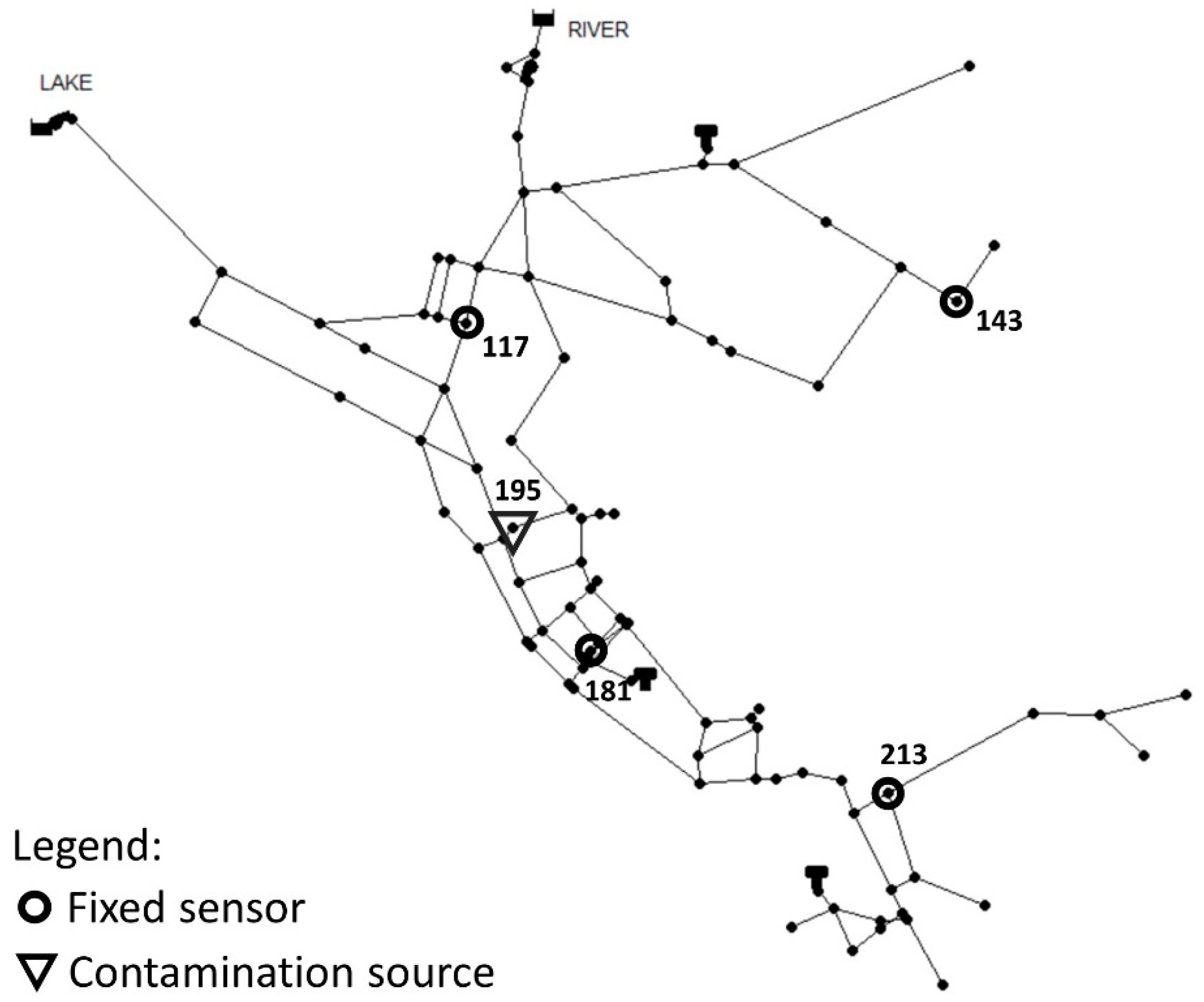
Figure 2 shows the two investigated fixed-sensor layouts. The left four-sensor layout was taken from [13] while the six-sensor layout on the right hand side of Figure 2 expands the former layout with two water quality sensors in strategically crucial nodes. The four-sensor layout included the nodes 117, 143, 181 and 213 while the six-sensor layout added the nodes 193 and 237.
The contamination scenarios were simulated assuming a single contamination node. All nodes were considered as possible contamination sources in the data generation process where the mass method was used for the injection characteristics. To increase the accuracy of the ANN, a vast amount of data needs to be generated. Therefore, in addition to using all system nodes as sources in the water quality simulations, the injection duration and concentration was also varied. The general simulation duration was 24 h where one hydraulic timestep represents one hour and the default quality timestep in WNTR of five minutes was adopted. Different start and end times of the contaminant injections were simulated, considering concentrations that ranged between 0.1 and 10 mg/L and that were continuously injected. The contamination concentration readings at the sensors are used as the data points to train the ANN. The all-zero readings were erased from the data.

2.4.2. The Artificial Neural Network

An artificial neural network is a supervised machine learning model that consists of an input layer, hidden layers and an output layer, which are all made up of interconnected neurons [45,49]. This deep learning model is a mathematical function that maps a specific set of input values to output values and is composed of many simpler functions [49]. While the authors in [16,47] used random forest algorithms to predict possible contamination sources and there are various real world applications for other algorithms such as K-nearest neighbour, support vector machines, decision trees or linear regression [50], this study chooses to use an ANN due to its capability to improve its performance with increasing amounts of data [50].
The ANN was created with the common open-source Python packages TensorFlow [51] and Scikit-learn [52]. The tuning of the hyperparameters of the ANN was performed with the KerasTuner package [53]. After the optimization of the ANN architecture and the hyperparameters for the four-sensor layout, the optimal ANN has 5 layers with 480 neurons in the first layer, 416 in the second layer, 512 in the third layer, 448 and 64 in the fourth and fifth layer respectively as seen in Table 1. The Adam optimizer was used with an optimal learning rate of 0.001. The categorical cross entropy loss function was used for the example. The rectified linear unit (reLu) is used as the activation function of the hidden layers and the softmax function was utilized for the output layer activation function. The optimal number of layers for the six-sensor layout was also five. The number of units per hidden layer were 448, 96, 288, 512 and 320 for layers one to five, respectively. The dropout values can be observed in Table 1. The dropout is a hyperparameter that can optimize the computational cost of the neural network by removing non-output units from the network by multiplying its output value with zero [49].
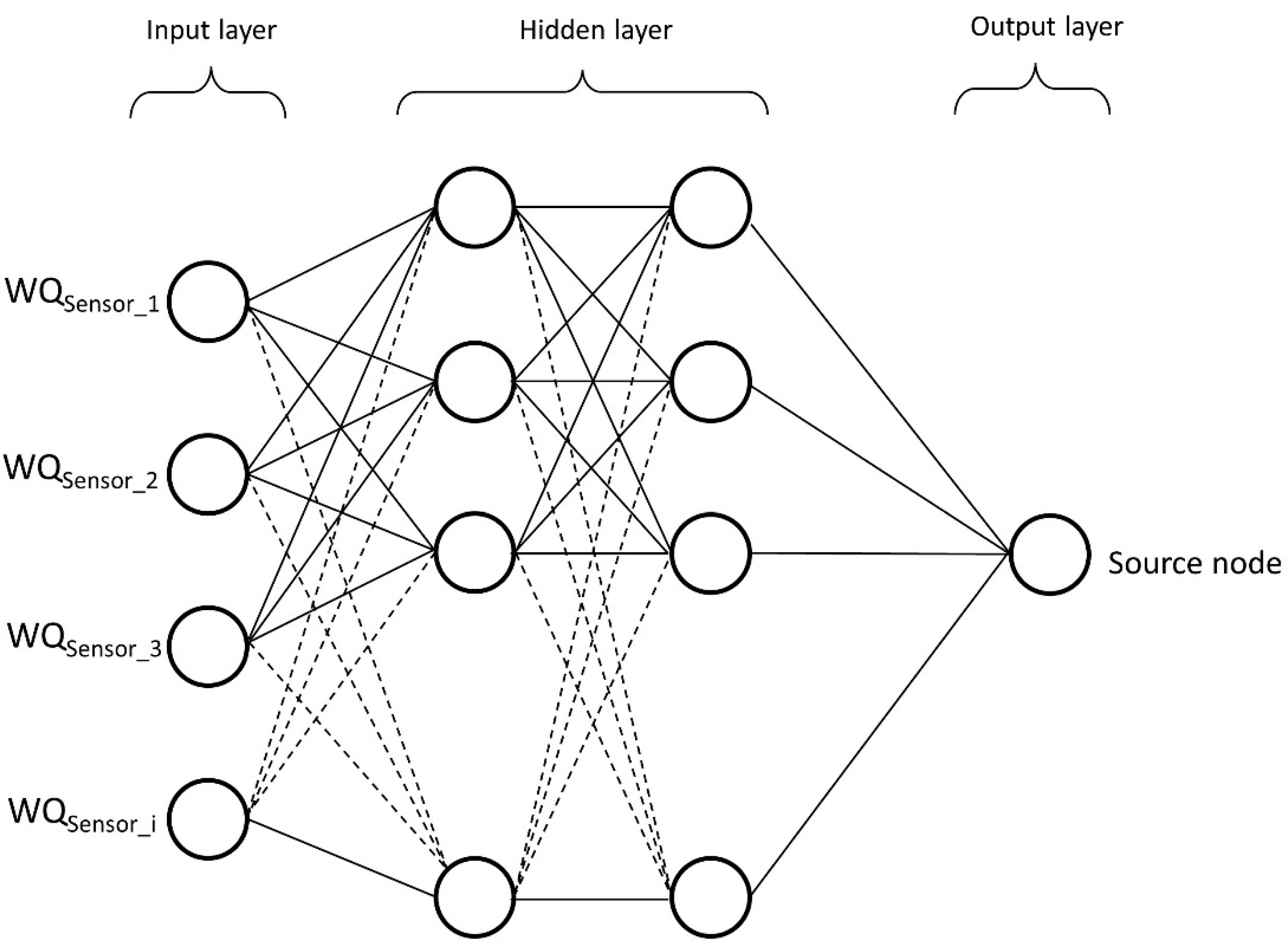
The neurons in the input layer have the same dimension as the number of sensors, i, as the sensor readings are the input features. The hidden layers help to approximate functions that are supposed to predict the source of the contamination. Every neuron in the hidden layer uses an assigned activation function to produce the individual output and is assigned a specific weight w. The output layer consists of a neuron that predicts the source node of the contamination with the following equation:
y ^ = f ( Z L ) ,
where y ^ is the prediction of the most probable source node, f the chosen activation function and ZL is the output of the last hidden layer:
Z L = Wi × A L 1 + b L ,
where W is the matrix representation of the weights of the individual neurons of the previous hidden layer; AL−1 the output of the previous hidden layer with L as the number of layers in the ANN; and bL represents the bias. Figure 3 shows the conceptual layout of the neural network where the water quality readings of the sensors are shown as the input features. The output layer uses the softmax function which determines the probability of the individual nodes being the source of the contamination. Therefore, the label dataset is encoded before the training of the neural network. The latter means that, in fact, the output of the ANN is a vector with 93 probabilities of being the source node of the contamination. The length of the vector corresponds to the number of nodes of the water network.

2.5. Placing Mobile Equipment

The objective for placing the mobile sensor equipment is for the utility manager to collect more information on the contamination spread in the water network upon the water anomaly detection. After a fixed sensor identifies the deterioration of water quality, the developed ANN will determine the most likely source node of the contamination. Subsequently, based on the flow directions within the water network, the endangered part of the WDS can be identified and one mobile sensor can be placed at every hydraulic timestep at another node downstream of the contamination to trace the contamination plume. The consumer agents can be warned about the network parts of the WDS that are endangered and about the regions that are not. This study uses deep learning and graph theory to identify the location for these mobile sensor locations.
The directed network Gc (Equation (4)) represents the possibly contaminated part of the water network where the contamination source is the actual source of that graph Gc, Nc represents the possibly contaminated terminal nodes and the edges Ec represent the
G c = { N c ,   E c ,   s = N cont } ,
where the source s of that graph is the source node of the contamination Ncont. Furthermore, the graph Gs represents the network part which is safe of the contamination, so every part of the network which is not part of Gc, as seen in Equation (5)
G s = { N s ,   E s } ,     G c ,  
Pipes where the direction of the graph Gc corresponds to the direction of flow where Ns and Es are the nodes and pipes/edges in which it is safe for the consumer agents to consume water.
The objective of the utility manager is to trace the contamination plume while informing and updating the consumers on the current status of contamination in the water network and minimizing the number of consumers that will be exposed to the contamination event. Equations (6)–(8) present the formulation to place the mobile sensor equipment:
minimize   C ex = f ABM   ( x , y ^ , t ) ,
Subject to:
x = x N ,   N     Z     ,  
t detection     t warn <   t clear ,   t ,   t warn   T s   ,  
where x represents the mobile equipment placement locations, twarn describes the time when the first warning about the contamination event is issued, tclear the timestep of complete clearance, Ts the complete time vector of the simulation and Cex the number of exposed consumers.

2.6. Issuing Warnings and Updates through Media Channels

Upon detection of the water quality anomaly, and identification of the source node and possibly endangered partitions of the water network, the utility manager communicates water advisories to the consumer agents. These advisories are general warnings about the status of the contamination according to the geographical location the consumers have in the water network. Ref. [9] describes how these warnings are being distributed among the consumer agents through traditional, and possibly social media, channels. The availability of the agents on the specific communication channels depends on their social background as does the communication amongst the agents themselves. As soon as the information reaches a consumer agent, the assumption is that their household will be informed during the next timestep of the simulation.

2.7. Consumer Agents

The consumer agents are split into three society types that are characterized by various variables that determine their social background. Table S1 shows the variables and values for the individual society types. If the consumers are informed about the water anomaly in their area of the network, they might change their consumer behaviour and reduce their water demands according to (9).
N 0 N n   D t + 1   = C t + 1 C t   ×   D t ,
where D is the demand in the respective timestep, C the number of consumers consuming drinking water and N the nodes in the network.

2.8. Social Background and Distribution in the Network

The classification of the social backgrounds was taken from [28]. The three society types are randomly distributed in the water network Net3 where Type 1 takes up 25% of the population, Type 2 45% and Type 3 10%. The geographical distribution of these types throughout the water network nodes is shown in Figure S1. Furthermore, the figure indicates areas in the network with different types such as industrial, residential or water utility nodes which make up the residual 20% of the water network nodes. The assumption of the distribution of the society types and the distribution of the state variables are loosely based on [28] and are assumed to be representative for a society in a medium sized community.

2.9. Fuzzy Logic for Determining Consumers’ Actions

The actions of the consumers were determined by utilizing fuzzy logic, which is contrary to Boolean logic where only false and true values (0 and 1, respectively) exist. This is a form of approximate reasoning with values between 0 and 1 and can be seen as a computational decision-making representation of e.g., humans [54,55]. The information on the social background of the consumers, their information status, etc. is represented in a fuzzy logic system as a membership function and with a predefined set of rules that framework can produce a defuzzified output of a crisp value that is processed by the agent-based framework. Therefore, the fuzzy set, A, can be represented as given in Equations (10) and (11):
A = { ( y , μ A ( y ) ) |   y     U }
μ A ( y )     [ 0 ,   1 ] ,
where y is an element in the fuzzy set, A, and µA(y) represents the membership of y in A.
The input values for the fuzzy logic systems are the location of the consumer agents, the social background variables, the agent’s information status on the networks’ contamination condition and the contamination consumption status. The fuzzy logic toolbox in MATLAB 2020a was utilized and integrated into the ABM. The output of the fuzzy logic is the probability of an individual consumer agent to take a specific action. For a more detailed explanation see [9].

3. Example Application

The water network system that was chosen for this application is the EPANET Net3 network (Figure 2). The system includes 92 nodes, two pumping stations, three tanks and two constant head sources and includes a 24-h demand pattern. The placement of the water quality sensors for the four-sensor layout is taken from [12], and are placed at nodes 117, 143, 181 and 213. The six-sensor layout expanded the four-sensor layout by placing two additional sensors at nodes 193 and 237 as shown in Figure 2.

3.1. Injection Scenario

The injection scenario was chosen randomly from the generated training dataset as described in Section 2.4.1. The variables for the injection were the start and end time of the contaminant injection, the contaminant concentration and the injection node. The EPANET source type was chosen as “mass” which adds a specific mass of species per unit of time to the flow entering the source node from all connecting pipes [42]. The contaminant injected is a non-specified pollutant and the simplified assumption is that the water quality sensors can measure the exact concentration of the contaminant. This assumption is considered appropriate for the proof of concept and can be expanded with more sophisticated water quality models in future work. The utility manager agent is alerted once a sensor measures any concentration of the contaminant in the WDS. Figure 4 shows an example of a random contamination scenario for the four-sensor layout. In this specific example, node 195 was randomly chosen to be the contamination source.

3.2. Mobile Equipment Placement

To place the mobile equipment sensor, a directed graph of the underlying EPANET Net3 network model needed to be created by utilizing the flow directions. The directed graph was created with MATLAB and the EPANET-MATLAB toolkit by considering all possible flow directions of the given demand patterns for the example network during the 24-h simulation. An adjacency matrix was generated by considering the flow directions of the water network and was used to create the directed network as can be seen in Figure 5. The nodes represent the demand nodes in the water network while the edges represent the respective flow directions. The need to consider all possible directions of the water flow is crucial because the flow directions for Net3 can vary over time as shown in Figure 5. The directed graph, which represents connectivity and all possible flow directions is crucial for assessing and identifying where the contaminant might spread throughout the duration of the simulation. Figure 5 also shows the fixed sensor locations as well as the contamination injection node at node 195. One mobile sensor is placed every other hydraulic timestep of the simulation at strategically important nodes downstream of the possible contamination source. The objective is to investigate the possibly contaminated partition of the water network Gc, which is represented by the red nodes in Figure 5, to either uphold the water advisory to the consumer agents or to clear them in case no imminent danger can be identified. If the specific water network is not considered endangered, those nodes can be assigned to the safe network subgraph Gs.
After contaminant detection at node 181, the ANN-based support tool identifies node 195 as the contamination source and the first mobile sensor is placed downstream at the edge of the network at node 169. The second and third placement iterations place additional mobile water quality sensors at nodes 199 and 237, respectively, which is the last part of the WDS in the branched Net3 network downstream of the contamination. This study will demonstrate the influence of the three mobile sensor placement iterations using the ANN source identification support tool on the response and recovery capabilities of the utility manager agent in case of a detected water quality anomaly.

3.3. Issuing Warnings to Consumer Agents

The utility manager warns the consumers about the contamination status of the WDS according to the information status of the plume spread. The water advisory is distributed through traditional and possibly social media channels. The specific dynamics of the availability and information distribution through social media is beyond the scope of this study, so necessary and appropriate assumptions were made. The consumers availability to the water advisory is based on their social background, in particular their employment status and their educational attainment. The information on the contamination status is assumed to be immediately transmitted to the consumer agents and based on their availability status. Once a consumer agent knows about their respective contamination status, they will inform their household in the next hydraulic timestep of the simulation. The information status is also used as an additional input into the fuzzy logic system for the decision making of the consumer agents.

3.4. Consumer Agent Actions

The consumer agent’s tendency to conduct certain actions is determined by the fuzzy logic system, which depends on the social background of the consumer agent, the information status, the location in the network and the possibility of the individual agent experiencing any symptoms from consuming contaminated drinking water. While in [9] the influence of these individual variables was investigated in different scenarios, this study utilizes all of these inputs at once in one scenario as the differentiation is not relevant for the main objective of this work.

3.5. Fuzzy Logic for Assigning Actions to Consumer Agents

The fuzzy logic system is implemented with the fuzzy logic toolbox of MATLAB 2020a. The variables of the individual agent (social background, etc.) are used in every timestep to determine the response of the agents considering a pre-defined set of rules and weights according to the assigned membership functions. The defuzzified output of the fuzzy logic systems are values between 0 and 1 and are used to determine whether the agents do not take an action, might possibly take an action or will take an action. The actions which were defined in [9] are the possibility of the agent to share right or wrong information about the spread, consult a physician, calling the water utility and changing their water demand behaviour. If the output Oan of the fuzzy logic system is smaller than 0.35 the specific action is not taken, if the values is between 0.35 and 0.65 the specific action is possibly taken and if the values is larger than 0.65 the specific action is taken.

4. Results

4.1. Accuracy of ANN to Determine the Contamination Source

The ANN-based source contamination identification system was thoroughly analysed for all possible contamination scenarios. The accuracy of the ANN was determined with the test set, which included twenty percent of the data. The generated data were shuffled before training the ANN to minimize variance and to guarantee the same data distribution over the training, validation, and test datasets. After training the model, the evaluation function of keras was used to determine the accuracy of the ANN in identifying the exact source of the contamination event. Furthermore, as done by the authors of [16], the accuracy of the model to identify the actual source node within the top 3, 5 or 10 most likely nodes was determined. The accuracy was determined with the keras evaluation function with a validation data split of 30%. This can be determined according to (12) and the results can be observed in Table 2.
A c c u r a c y = P r c P r t o t
where Prc represents the sum of the cases where the ANN predicted the correct source node and Prtot the total sum of predictions. For the case of the top 3, 5 or 10 nodes, Prc is determined by checking whether the maximum n (3, 5 or 10) probabilities of the neural network output, which is a vector of 97 nodes, is the actual contamination source node. The accuracy of the ANN to identify the exact contamination source for any given contamination event for a four-sensor layout is quite low with 48.2% and does not serve as a reliable support tool for the utility manager to determine where a possibly water quality anomaly is originating. Although the accuracy for determining the exact source with a six-sensor layout shows significant improvement at 60.8%, that the system does not identify the source contamination in almost 40% of the cases is problematic. When considering at the top n prediction accuracies there are already major improvements in accuracy for both sensor layouts. For the four-sensor layout the ANN can reach almost 70% accuracy in identifying the correct source node, while the accuracy for the top 10 cases of the six-sensor layout is 79.8%. From a practical engineering point of view, the installation of two additional sensors in the water network, and subsequently collecting more data and receiving more input, generated an improvement in the accuracy of the ANN by 10%. Finally, the accuracy of identifying the actual contamination source within the top 3 most likely contamination sources, instead of just using the most likely source node, significantly improved the accuracy. The increased accuracy was particularly good for the six-sensory layout with an increase in accuracy to 72.5% that can give satisfactory support to the utility manager in determining where the mobile sensors can be placed upon detection of the water event.

4.2. Source Prediction and Mobile Sensor Placement

For these results, the example of Figure 5 with a four-sensor layout and a source prediction of the most likely top three nodes was used. The trained ANN model was given the water quality values of the sensors as an input to determine the source node of the contamination after a water quality anomaly was initially detected at node 181. The node where the contaminant was injected in this randomly selected case was at node 195, as indicated in Figure 5. Since the placement of additional mobile sensors is dependent on the identification of the source location, two prediction scenarios of the possible sources are presented to demonstrate the challenges presented to a utility manager. The first scenario (Figure 6) represents a prediction where the source was determined with a high probability. The second scenario (Figure 7) presents a prediction where the ANN puts out a similar probability to the top three most likely nodes to be the contamination source. For both scenarios, as the contamination spread downstream, the fixed sensors at nodes 117 and 143 did not measure any changing water quality parameters.
The first scenario, presented in Figure 6, represents a prediction where the actual source was predicted to be the source (node 195) with a high probability of 95%, where the second (4%) and third highest (1%) probabilities were assigned to the Nodes 601 and 153, respectively. The probability values are rounded and may not add up to a hundred percent (e.g., Figure 7). The utility manager uses the knowledge of the network topology, possible flow directions, and placement of the other fixed sensors as additional information to further determine the contamination source probability. Figure 6 shows all possible flow directions in Net3 as well as the locations of the possible sources and the four fixed water quality sensors. The fixed sensors in the nodes 117 and 143 are downstream of the possible source nodes 601 and 153, respectively, and these water quality sensors did not record any readings of water anomalies which further decreases the probability of these sources to be the actual contamination source. The output of the ANN support tool, as well as the topological and hydraulic information on the network, presents the utility manager with the contamination source location, node 195, with a very high certainty and accuracy, which must be examined apart from the accuracy of the neural network.
The second prediction scenario from the ANN-based support tool output is presented in Figure 7. As in Figure 6, this is a graphical representation of the Net3 network including all possible flow directions, the fixed sensor positions and the top three possible source nodes. In this scenario, the determination of the actual source was not as obvious as in the first case. The probabilities for nodes 195, 191, and 187 to be the contamination source are 34%, 34% and 30%, respectively. As the nodes are all in direct proximity to one another, the similarly distributed probabilities for the top three most likely nodes makes sense and does give a good indication as to how much the data-driven system understands the actual hydraulics. Similarly, as shown for the first prediction case, the utility manager decision needs to be based on the hydraulic and topological network system. Furthermore, in case there is not enough certainty about the verified contamination source, the worst case needs to be assumed. In case of the presented second prediction scenario, nodes 191 and 187 are effectively “downstream” of the node 195. Therefore, the number of possibly contaminated nodes is larger and the possibilities of geographical spread are higher. This justifies the worst-case assumption that the node 195 is the source node, and the placement of the mobile sensor equipment needs to be adjusted to include that worst-case assumption.
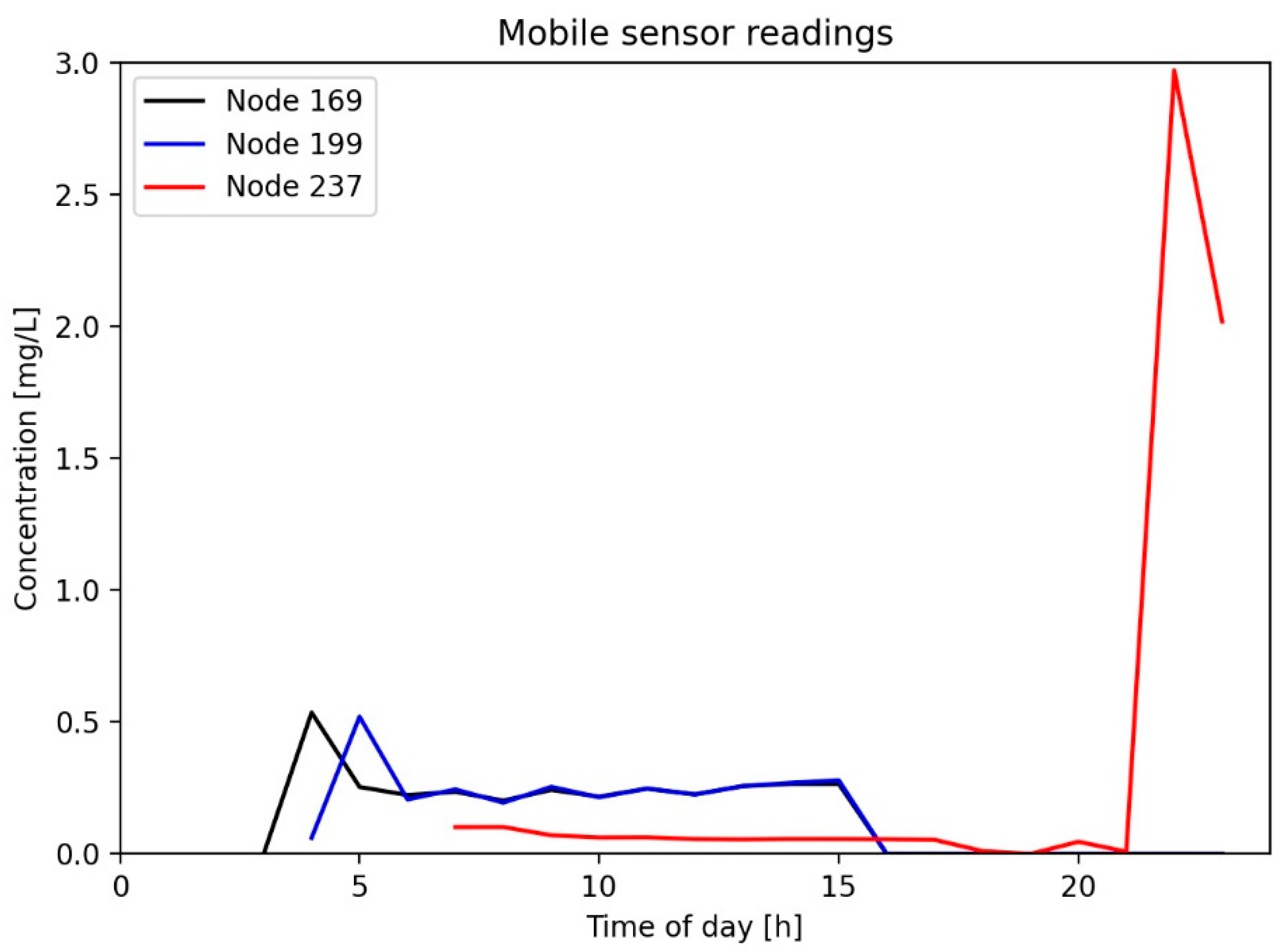
The sensor placement was conducted as explained in Section 3.2 and visualised with Figure 5. After discovering the water quality anomaly initially at node 181 at hour one of the 24-h simulation and determining that the contamination source for both prediction cases is node 195, the utility manager places mobile sensor equipment every other hour. The sensor placement is conducted in three iterations. On the first iteration the first sensor is placed at node 169, the second sensor is placed at node 199 and the third sensor is placed at node 237 for the last iteration. Figure 8 shows the respective water quality readings for the mobile sensors starting at the hour the mobile sensors are placed. The observed concentrations for the mobile sensors at nodes 169 and 199 peak with a time shift that can be explained by the location of the second sensor being further downstream of node 199. The specific contamination case, which was chosen here, has a duration of ten hours, starting at hour zero. So, the sensors at nodes 169 and 199 maintain a stable concentration of around 0.3 mg/L until about five hours after the injection stops and the concentrations drop back to 0. Therefore, the contamination remains in the higher middle region of the branched Net3 system for around five hours after the injection stops. While the water quality sensor at Node 237 just detects minor amounts of concentration throughout the first 21 h of the simulation, the concentration dramatically peaks up to 3 mg/L, which indicates that the demand pattern changes in the evening hours and that spread the remnants of the injected contaminant into the last cluster of the branched network.

4.3. Water Advisories and Reaction of Consumer Agents

After the source prediction, mobile sensor placement and evaluation of the water quality readings, the part of the water network upstream of the contamination source (blue nodes in Figure 5) can be declared as non-endangered of being contaminated. In the initial step, the non-endangered information is communicated to the consumer agents by the utility manager. For the rest of the system, a water advisory is announced and remains intact until the contaminant concentration at nodes 169 and 199 drops at around hour 16. Then, assuming the source has been verified and the injection has stopped, nodes upstream of 199 are declared as safe by the utility manager as well and the water advisory is updated. The water advisory for the lower cluster of nodes downstream of 199 will be maintained until the end of the simulation period as there are still high concentration readings at node 237.
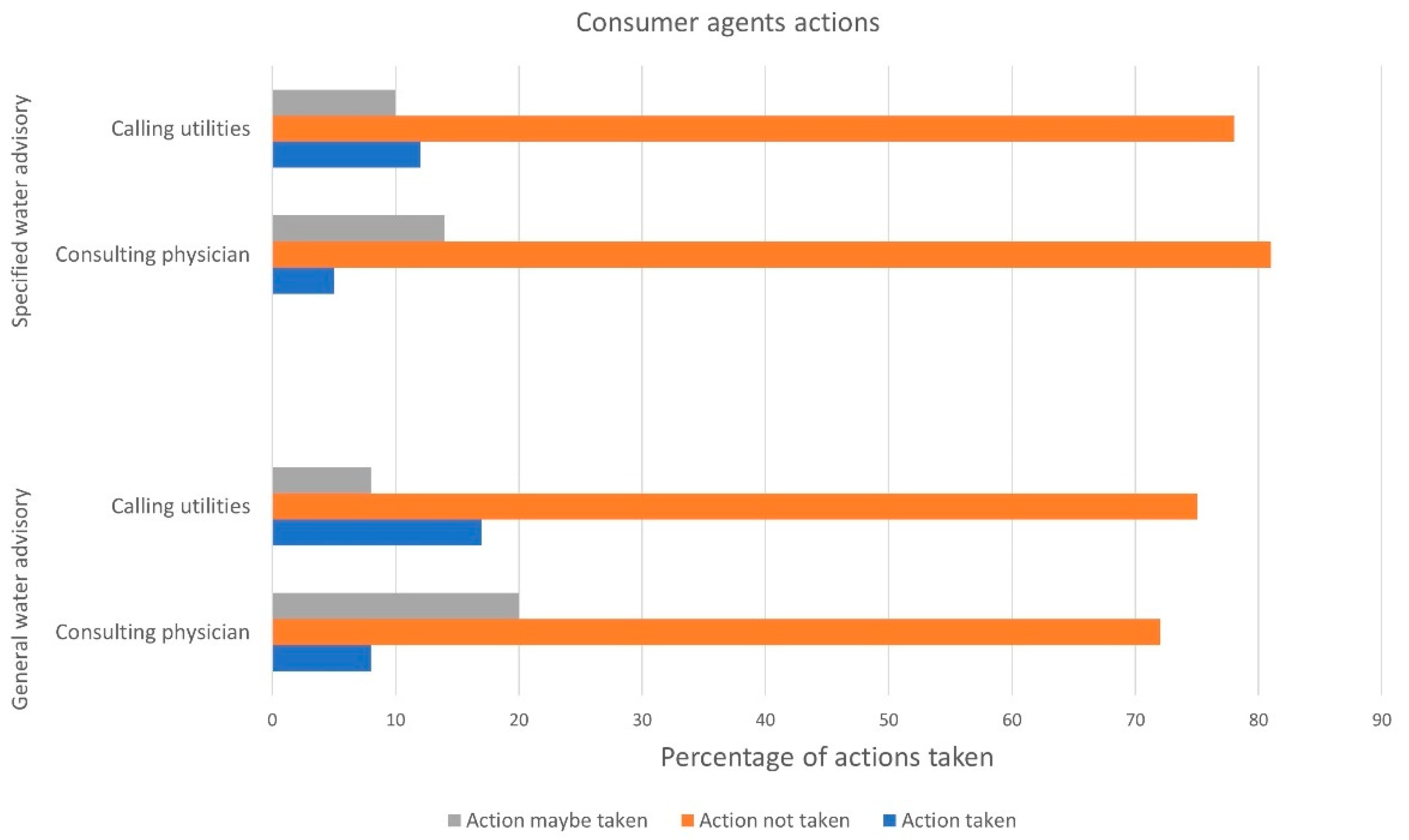
For this study, two possible actions by the consumer agents are highlighted in the results. The possibility of calling the utility or consulting a physician by the consumer agents are analysed for two scenarios. The first scenario, which is based on the built agent-based framework from [9], involves a water advisory from the utility manager that is very general and non-specific to the actual contamination spread in the water network. The second scenario considers a specific water advisory that updates the consumer agents about the current status of the contamination of their physical location. After placing the mobile sensor equipment and investigating the spread of the contamination, the utility manager updates the water advisory specific to which part of the network is safe and which part is endangered. Figure 9 shows the bar diagram that represents the consumer agents‘ actions for the general and specific water advisories, which is given by the fuzzy logic systems output. As the variables for the fuzzy logic system responsible for the decision-making process depend on the location of the consumer agents, the information status of the agent is crucial. For the specific water advisory, the number of agents that decide to contact the water utilities or consult a physician has decreased in comparison to the general water advisory. The number of agents that will maybe take one of these two actions is smaller for the geographically specific water advisory and the percentage of agents that will not take any actions decreases accordingly. As the utility manager monitors the relevant parts of the water network with mobile sensor equipment and can update the consumers about the current status of the network, the number of agents which are endangered, or possibly endangered, has significantly decreased.

5. Conclusions

Previously conducted studies have investigated the placement of fixed or inline water quality sensors and source identification via machine learning in a water network with the consideration of a possible water contamination event. Furthermore, various agent-based modelling frameworks have been used to simulate disastrous and hazardous situations, specifically for events of water quality deterioration. A variety of these frameworks consider psychological models or surveys to determine the reaction of agents; particularly due to recent events, events which have prompted a closer focus on how the agents might have changed during the global COVID-19 pandemic. This study suggests a novel response-and-recovery method for contamination events in water networks that utilizes machine learning, as well exploring an approach that draws on a COVID-19 inspired agent-based modelling (ABM) framework. The ABM was written from scratch in MATLAB and coupled with the EPANET hydraulic simulator through the EPANET-MATLAB toolkit. The utilization of a non-proprietary software for building the ABM model facilitated a very flexible handling of the framework. Moreover, the data generation and training of the neural networks was conducted with Python packages such as WNTR, Keras, TensorFlow and scikit-learn. The ABM simulates consumer agents, that ingest water from the water network, communicate with each other and share information on the contamination status, and a utility manager who is responsible for reacting to the water event once an anomaly is detected. The utility manager agent can place mobile sensor equipment to trace the contamination spread downstream and utilizes an artificial neural network (ANN) based support tool for source identification. The ANN is built and trained to determine the source of any given water contamination based on the readings of fixed water quality sensors. The neural network is trained with water quality simulation data from a four-sensor and six-sensor layout in an EPANET network system. Based on the information the utility manager is receiving from mobile sensor equipment, the consumer agents are informed about the current contamination status based upon their geographical location in the network and react by, e.g., calling the utilities or consulting a physician.
An application example was presented where a four-sensor layout was investigated for a random contamination event in the water network. The ANN support tool for the source identification predicts the probability of the top three most likely contamination sources upon initial detection of the contamination. Two prediction scenarios were evaluated. One scenario where the ANN resulted in a high probability for one single node and a second scenario where three nodes were predicted as possible sources with almost equally distributed probabilities. By utilizing the topological and hydraulic information of the network, the source of the contamination can be identified with higher certainty. The accuracy of the neural network system increases with more sensors and data, and when determining the probabilities of the top three, five or ten most likely nodes to be the source of the contamination instead of just one node. The developed framework is suitable to balance possible accuracy weaknesses of the ANN by utilizing graph theory and considering all possible flow directions for identifying whether a predicted source can physically be the contamination source. Upon contamination detection, mobile sensor equipment was placed in strategically crucial places downstream of the detected source. Using the additional sensor readings, the current contamination status was communicated to the consumer agents. The responses demonstrate that, with a specific water advisory in which the actual endangered nodes of the system are considered, the consumer agents tended to seek help less and were engaging their physicians or water utilities less. These results suggest that by identifying the realistically endangered nodes in the water network, there can be benefits for, e.g., the water utility operation as well as for the infrastructure as the demands of the consumers would change in a less dramatic way. This study has shown that contamination response and recovery is a holistic problem and needs to be treated as such. Addressing all stakeholders’ possible actions and reactions as well as taking into account all possible contamination scenarios is essential when responding to an event. While other studies used purely data-driven models to determine the contamination source during a water event, the contribution of this study is the utilization of the knowledge on the network topology and the system hydraulics as well. Finding a possibility to use the available water quality data in a hybrid data-driven model that can be optimized with the knowledge on the actual physical system can save computing power and provide more certainty as a support tool to the utility manager of a WDS. This framework can be expanded and applied to other, more complex water networks where even more data can be generated to train the ANN.
Future work should explore a more complex interaction and social network system of the consumer agents, which was beyond the scope of this research. Additional surveys can be conducted, and more sophisticated psychological models involved to validate the behaviour of the consumer agents. Furthermore, the mobility of the agents in between the water network nodes can be considered as part of an expansion of this study. Particularly given how global shut-down orders and the change of routines for major parts of the population since the global COVID-19 pandemic have started.
Considering that the network Net3 which is used in this study is a relatively small network, the obtained amount of data points from the water quality simulations is very substantial. This framework will be applied to water networks with higher complexities and the performance of the ANN is expected to increase with large amounts of data. Nevertheless, a sensitivity analysis on various other machine learning algorithms and their suitability for the problem of the source identification should be conducted. Support vector machines and random forest algorithms could be utilized and their hyperparameters tuned to predict the possible source of the contamination. While the ANN paired with graph theory performed well to predict the top three five or ten most likely contamination source nodes, the aim should be to find a methodology to predict the exact source node with very high accuracy and certainty.

Supplementary Materials

The following supporting information can be downloaded at: https://www.mdpi.com/article/10.3390/w14071088/s1, Figure S1: Distribution society types; Table S1: Variables social background.

Author Contributions

Conceptualisation, L.K., E.B. and A.O.; methodology, L.K., C.S., D.L.B., E.B. and A.O.; writing—original draft preparation, L.K.; writing—review and editing, L.K., C.S., D.L.B., E.B. and A.O.; supervision, A.O.; project Administration, D.L.B. and A.O.; funding acquisition, D.L.B. and A.O. All authors have read and agreed to the published version of the manuscript.

Funding

This research was supported by a grant from the United States–Israel Binational Science Foundation (BSF), Jerusalem, Israel.

Institutional Review Board Statement

Not applicable.

Informed Consent Statement

Not applicable.

Data Availability Statement

The data presented in this study are available on request from the corresponding author.

Acknowledgments

This research was supported by a grant from the United States–Israel Binational Science Foundation (BSF).

Conflicts of Interest

The authors declare no conflict of interest.

References

  1. Janke, R.; Murray, R.; Uber, J.; Taxon, T. Comparison of Physical Sampling and Real-Time Monitoring Strategies for Designing a Contamination Warning System in a Drinking Water Distribution System. J. Water Resour. Plan. Manag. 2006, 132, 310–314. [Google Scholar] [CrossRef]
  2. Hall, J.; Zaffiro, A.D.; Marx, R.B.; Kefauver, P.C.; Radha Krishnan, E.; Haught, R.C.; Herrmann, J.G. On-line water quality parameters as indicators of distribution system contamination. J. Am. Water Work. Assoc. 2007, 99, 66–77. [Google Scholar] [CrossRef]
  3. Ostfeld, A.; Salomons, E. Optimal layout of early warning detection stations for water distribution systems security. J. Water Resour. Plan. Manag. 2004, 130, 377–385. [Google Scholar] [CrossRef]
  4. Ostfeld, A.; Über, J.G.; Salomons, E.; Berry, J.W.; Hart, W.E.; Phillips, C.A.; Watson, J.P.; Dorini, G.; Jonkergouw, P.; Kapelan, Z.; et al. The battle of the water sensor networks (BWSN): A design challenge for engineers and algorithms. J. Water Resour. Plan. Manag. 2008, 134, 556–568. [Google Scholar] [CrossRef] [Green Version]
  5. Wu, L.; Wan Salim, W.W.A.; Malhotra, S.; Brovont, A.; Park, J.H.; Pekarek, S.D.; Banks, M.K.; Porterfield, D.M. Self-powered mobile sensor for in-pipe potable water quality monitoring. In Proceedings of the 17th International Conference on Miniaturized System for Chemistry and Life Science, MicroTAS 2013, Freiburg, Germany, 27–31 October 2013; Volume 1, pp. 14–16. [Google Scholar]
  6. Sankary, N.; Ostfeld, A. Inline mobile sensors for contaminant early warning enhancement in water distribution systems. J. Water Resour. Plan. Manag. 2017, 143, 04016073. [Google Scholar] [CrossRef]
  7. Sankary, N.; Ostfeld, A. Multiobjective optimization of inline mobile and fixed wireless sensor networks under conditions of demand uncertainty. J. Water Resour. Plan. Manag. 2018, 144, 04018043. [Google Scholar] [CrossRef]
  8. Kadinski, L.; Rana, M.; Boccelli, D.; Ostfeld, A. Water Distribution Systems Analysis. In Proceedings of the World Environmental and Water Resources Congress 2019; American Society of Civil Engineers: Reston, VA, USA, 2019; pp. 536–542. [Google Scholar]
  9. Kadinski, L.; Ostfeld, A. Incorporation of COVID-19-Inspired Behaviour into Contamination Responses. Water 2021, 13, 2863. [Google Scholar] [CrossRef]
  10. Asheri Arnon, T.; Ezra, S.; Fishbain, B. Water characterization and early contamination detection in highly varying stochastic background water, based on Machine Learning methodology for processing real-time UV-Spectrophotometry. Water Res. 2019, 155, 333–342. [Google Scholar] [CrossRef]
  11. Ashwini, C.; Singh, U.P.; Pawar, E. Shristi Water quality monitoring using machine learning and iot. Int. J. Sci. Technol. Res. 2019, 8, 1046–1048. [Google Scholar]
  12. Preis, A.; Ostfeld, A. A contamination source identification model for water distribution system security. Eng. Optim. 2007, 39, 941–947. [Google Scholar] [CrossRef]
  13. Taylor, P.; Preis, A.; Ostfeld, A. Civil Engineering and Environmental Systems Genetic algorithm for contaminant source characterization using imperfect sensors. Civ. Eng. Environ. Syst. 2008, 25, 37–41. [Google Scholar] [CrossRef]
  14. Kim, M.; Choi, C.Y.; Gerba, C.P. Source tracking of microbial intrusion in water systems using artificial neural networks. Water Res. 2008, 42, 1308–1314. [Google Scholar] [CrossRef] [PubMed] [Green Version]
  15. Lee, Y.J.; Park, C.; Lee, M.L. Identification of a Contaminant Source Location in a River System Using Random Forest Models. Water 2018, 10, 391. [Google Scholar] [CrossRef] [Green Version]
  16. Grbčić, L.; Lučin, I.; Kranjčević, L.; Družeta, S. Water supply network pollution source identification by random forest algorithm. J. Hydroinform. 2020, 22, 1521–1535. [Google Scholar] [CrossRef]
  17. Shafiee, M.E.; Berglund, E.Z. Complex adaptive systems framework to simulate the performance of hydrant flushing rules and broadcasts during a water distribution system contamination event. J. Water Resour. Plan. Manag. 2017, 143, 04017001. [Google Scholar] [CrossRef]
  18. Bonabeau, E. Agent-based modeling: Methods and techniques for simulating human systems. Proc. Natl. Acad. Sci. USA 2002, 99, 7280–7287. [Google Scholar] [CrossRef] [Green Version]
  19. Athanasiadis, I.N.; Mentes, A.K.; Mitkas, P.A.; Mylopoulos, Y.A. A Hybrid Agent-Based Model for Estimating Residential Water Demand. Simulation 2005, 81, 175–187. [Google Scholar] [CrossRef] [Green Version]
  20. Linkola, L.; Andrews, C.J.; Schuetze, T. An agent based model of household water use. Water 2013, 5, 1082–1100. [Google Scholar] [CrossRef]
  21. Ding, N.; Erfani, R.; Mokhtar, H.; Erfani, T. Agent based modelling forwater resource allocation in the transboundary Nile river. Water 2016, 8, 139. [Google Scholar] [CrossRef]
  22. Tillman, D.E.; Larsen, T.A.; Pahl-Wostl, C.; Gujer, W. Simulating development strategies for water supply systems. J. Hydroinform. 2005, 7, 41–51. [Google Scholar] [CrossRef] [Green Version]
  23. Ehsan Shafiee, M.; Zechman, E.M. An agent-based modeling framework for sociotechnical simulation of water distribution contamination events. J. Hydroinform. 2013, 15, 862–880. [Google Scholar] [CrossRef] [Green Version]
  24. Shafiee, M.E.; Berglund, E.Z.; Lindell, M.K. An Agent-based Modeling Framework for Assessing the Public Health Protection of Water Advisories. Water Resour. Manag. 2018, 32, 2033–2059. [Google Scholar] [CrossRef]
  25. Monroe, J.; Ramsey, E.; Berglund, E. Allocating countermeasures to defend water distribution systems against terrorist attack. Reliab. Eng. Syst. Saf. 2018, 179, 37–51. [Google Scholar] [CrossRef]
  26. Zechman, E.M. Agent-based modeling to simulate contamination events and evaluate threat management strategies in water distribution systems. Risk Anal. 2011, 31, 758–772. [Google Scholar] [CrossRef]
  27. Kennedy, W.G. Modelling Human Behaviour in Agent-Based Models. In Agent-Based Models of Geographical Systems; Springer: Dordrecht, The Netherlands, 2012; pp. 167–179. ISBN 9789048189274. [Google Scholar]
  28. Wang, C.; Pan, R.; Wan, X.; Tan, Y.; Xu, L.; Ho, C.S.; Ho, R.C. Immediate psychological responses and associated factors during the initial stage of the 2019 coronavirus disease (COVID-19) epidemic among the general population in China. Int. J. Environ. Res. Public Health 2020, 17, 1729. [Google Scholar] [CrossRef] [Green Version]
  29. Pennycook, G.; McPhetres, J.; Zhang, Y.; Rand, D. Fighting COVID-19 misinformation on social media: Experimental evidence for a scalable accuracy nudge intervention. PsyArXiv Working Pap. 2020, 31, 770–780. [Google Scholar] [CrossRef]
  30. Van Bavel, J.J.; Baicker, K.; Boggio, P.S.; Capraro, V.; Cichocka, A.; Cikara, M.; Crockett, M.J.; Crum, A.J.; Douglas, K.M.; Druckman, J.N.; et al. COVID-19 pandemic response. Nat. Hum. Behav. 2020, 4, 460–471. [Google Scholar] [CrossRef]
  31. Spearing, L.A.; Thelemaque, N.; Kaminsky, J.A.; Katz, L.E.; Kinney, K.A.; Kirisits, M.J.; Sela, L.; Faust, K.M. Implications of Social Distancing Policies on Drinking Water Infrastructure: An Overview of the Challenges to and Responses of U.S. Utilities during the COVID-19 Pandemic. ACS ES&T Water 2021, 1, 888–899. [Google Scholar] [CrossRef]
  32. Maziarz, M.; Zach, M. Agent-based modelling for SARS-CoV-2 epidemic prediction and intervention assessment: A methodological appraisal. J. Eval. Clin. Pract. 2020, 26, 1352–1360. [Google Scholar] [CrossRef]
  33. Silva, P.C.L.; Batista, P.V.C.; Lima, H.S.; Alves, M.A.; Guimarães, F.G.; Silva, R.C.P. COVID-ABS: An agent-based model of COVID-19 epidemic to simulate health and economic effects of social distancing interventions. Chaos Solitons Fractals 2020, 139, 110088. [Google Scholar] [CrossRef]
  34. Sullivan, G.L.; Delgado-Gallardo, J.; Watson, T.M.; Sarp, S. An investigation into the leaching of micro and nano particles and chemical pollutants from disposable face masks-linked to the COVID-19 pandemic. Water Res. 2021, 196, 117033. [Google Scholar] [CrossRef] [PubMed]
  35. Bussan, D.D.; Snaychuk, L.; Bartzas, G.; Douvris, C. Quantification of trace elements in surgical and KN95 face masks widely used during the SARS-COVID-19 pandemic. Sci. Total Environ. 2022, 814, 151924. [Google Scholar] [CrossRef] [PubMed]
  36. Saberi-Movahed, F.; Mohammadifard, M.; Mehrpooya, A.; Rezaei-Ravari, M.; Berahmand, K.; Rostami, M.; Karami, S.; Najafzadeh, M.; Hajinezhad, D.; Jamshidi, M.; et al. Decoding Clinical Biomarker Space of COVID-19: Exploring Matrix Factorization-Based Feature Selection Methods. MedRxiv 2021. [Google Scholar] [CrossRef]
  37. Luo, J.; Zhou, L.; Feng, Y.; Li, B.; Guo, S. The selection of indicators from initial blood routine test results to improve the accuracy of early prediction of COVID-19 severity. PLoS ONE 2021, 16, e0253329. [Google Scholar] [CrossRef]
  38. Karthikeyan, A.; Garg, A.; Vinod, P.K.; Priyakumar, U.D. Machine Learning Based Clinical Decision Support System for Early COVID-19 Mortality Prediction. Front. Public Health 2021, 9, 626697. [Google Scholar] [CrossRef]
  39. Helbing, D.; Farkas, I.; Vicsek, T. Simulating dynamical features of escape panic. Nature 2000, 407, 487–490. [Google Scholar] [CrossRef] [Green Version]
  40. Eliades, D.G.; Kyriakou, M.; Vrachimis, S.; Polycarpou, M.M. EPANET-MATLAB Toolkit: An Open-Source Software for Interfacing EPANET with MATLAB. In Proceedings of the Computer Control for Water Industry (CCWI), Amsterdam, The Netherlands, 7–9 November 2016; pp. 1–8. [Google Scholar] [CrossRef]
  41. Rossman, L. Epanet 2 Users Manual; U.S. Environmental Protection Agency: Washington, DC, USA, 2000.
  42. Shang, F.; Uber, J.G. Epanet Multi-Species Extension User’ S Manual; U.S. Environmental Protection Agency: Washington, DC, USA, 2011.
  43. He, K.; Zhang, X.; Ren, S.; Sun, J. Deep Residual Learning for Image Recognition. In Proceedings of the Computer Vision and Pattern Recognition (CVPR), Las Vegas, NV, USA, 27–30 June 2016. [Google Scholar]
  44. Kashani, S. Deep Learning Interviews: Hundreds of fully Solved Job Interview Questions from a Wide Range of Key Topics in AI; Published by Shlomo Kashani, Tel-Aviv, ISRAEL; Cornell University: Ithaca, NY, USA, 2020; ISBN 1916243568. [Google Scholar]
  45. Fan, X.; Zhang, X.; Yu, X.B. Machine learning model and strategy for fast and accurate detection of leaks in water supply network. J. Infrastruct. Preserv. Resil. 2021, 6, 10. [Google Scholar] [CrossRef]
  46. Mashhadi, N.; Shahrour, I.; Attoue, N.; Khattabi, J. El smart cities Use of Machine Learning for Leak Detection and Localization in Water Distribution Systems. Smart Cities 2021, 4, 1293–1315. [Google Scholar] [CrossRef]
  47. Grbčić, L.; Kranjčević, L.; Družeta, S. Machine Learning and Simulation-Optimization Coupling for Water Distribution Network Contamination Source Detection. Sensors 2021, 21, 1157. [Google Scholar] [CrossRef]
  48. Klise, K.A.; Hart, D.; Moriarty, D.; Bynum, M.L.; Murray, R.; Burkhardt, J.; Haxton, T. Water Network Tool for Resilience (WNTR) User Manual Disclaimer; U.S. Environmental Protection Agency: Washington, DC, USA, 2017; pp. 59–64.
  49. Goodfellow, I.; Bengio, Y.; Courville, A. Deep Learning; MIT Press: Cambridge, MA, USA, 2016. [Google Scholar]
  50. Sarker, I.H. Deep Learning: A Comprehensive Overview on Techniques, Taxonomy, Applications and Research Directions. SN Comput. Sci. 2021, 2, 420. [Google Scholar] [CrossRef]
  51. Abadi, M.; Agarwal, A.; Barham, P.; Brevdo, E.; Chen, Z.; Citro, C.; Corrado, G.S.; Davis, A.; Dean, J.; Devin, M.; et al. TensorFlow: Large-Scale Machine Learning on Heterogeneous Systems. arXiv 2016, arXiv:1603.04467. [Google Scholar]
  52. Pedregosa, F.; Weiss, R.; Brucher, M. Scikit-learn: Machine Learning in Python. J. Mach. Learn. Res. 2011, 12, 2825–2830. [Google Scholar]
  53. O’Malley, T.; Bursztein, E.; Long, J.; Chollet, F. KerasTuner. Retrieved May 2019, 21, 2020. [Google Scholar]
  54. Zadeh, L.A. Fuzzy sets. Inf. Control 1965, 8, 338–353. [Google Scholar] [CrossRef] [Green Version]
  55. Gerla, G. Effectiveness and multivalued logics. J. Symb. Log. 2006, 71, 137–162. [Google Scholar] [CrossRef]
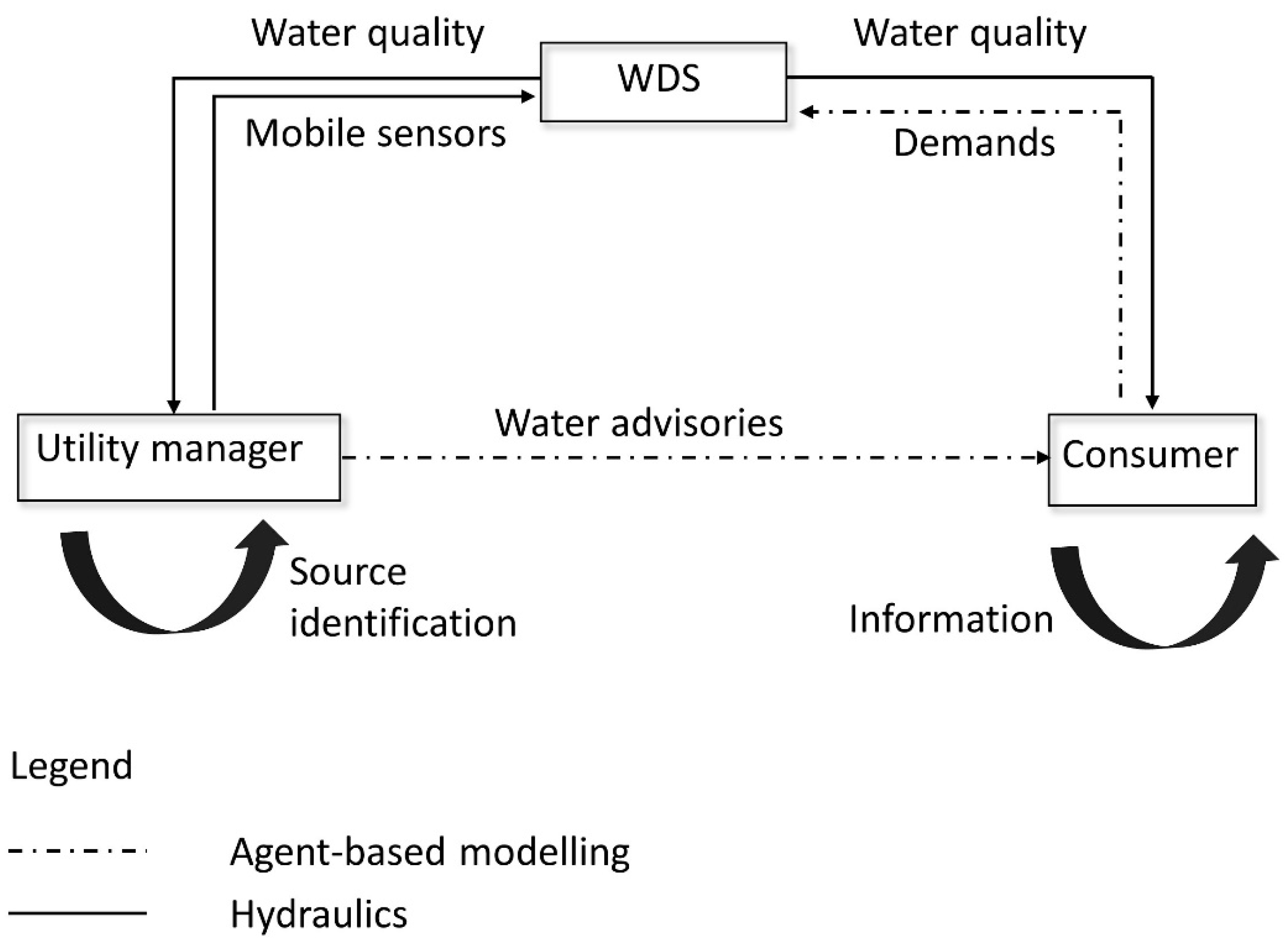
Figure 1. Conceptual flowchart of the agent-based modelling framework.
Water 14 01088 g001
Figure 2. Layouts of fixed water quality sensors. On the left, a four-sensor layout taken from [12]. On the right, a six-sensor layout which expands the left layout by two additional strategically placed water quality sensor.
Water 14 01088 g002
Figure 3. Conceptual layout of the ANN for the framework to determine the possible source of a contamination in a WDS.
Water 14 01088 g003
Figure 4. EPANET Net3 example network including the locations of the four-sensor layout system with sensors at the nodes 117, 143, 181 and 213 and the contamination injection node 195.
Water 14 01088 g004
Figure 5. Directed graph of Net3 network depicting all possible flow directions that can occur over a 24 h demand period including the positions of the fixed water quality sensors, the contamination source, the placement of the mobile sensor equipment for the first three iteration and the network clusters which are considered endangered Gc, and which can be declared safe Gs.
Water 14 01088 g005
Figure 6. Directed graph of Net3 including all possible flow directions and the positions of the fixed sensors, the first contamination detection (node 181), and the prediction of the top three most likely nodes including the probability of these nodes being the contaminant source. This figure represents the first prediction scenario with a clear distinction of the prediction probabilities.
Water 14 01088 g006
Figure 7. Directed graph of Net3 including all possible flow directions and the positions of the fixed sensors, the first contamination detection (node 181), and the prediction of the top three most likely nodes including the probability of these nodes being the contaminant source. This figure represents the second prediction scenario without a clear distinction of the prediction probabilities.
Water 14 01088 g007
Figure 8. Mobile sensor readings at nodes 169, 199 and 237. Each reading starts time delayed, after their placement in the first, second and third iteration respectively.
Water 14 01088 g008
Figure 9. Bar diagram to represent the consumer agents’ actions taken for a general water advisory without any information on the exact geographical spread and a specified water advisory which includes the utility manager updating the consumer agents about the current contamination status of their location. Specifically, whether the consumer agents call the water utilities or consult a physician.
Water 14 01088 g009
Table 1. Summary of ANN Algorithm and Architecture Hyperparameters.
HyperparameterFour-Sensor LayoutSix-Sensor Layout
Layer number55
Learning rate0.00010.0001
Unit 1480448
Dropout unit 100.1
Unit 241696
Dropout unit 200
Unit 3512288
Dropout unit 30.10
Unit 4448512
Dropout unit 40.10.1
Unit 564320
Dropout unit 50.10.2
Table 2. Accuracy of Artificial Neural Network for the Four- And Six-Sensor Layouts for Determining the Exact Source Node or the 3, 5 or 10 Most Likely Nodes.
ANN AccuracyFour-Sensor LayoutSix-Sensor Layout
Exact source48.2%60.8%
Top 361.8%72.5%
Top 566.0%76.7%
Top 1069.8%79.8%
Publisher’s Note: MDPI stays neutral with regard to jurisdictional claims in published maps and institutional affiliations.