
Effect of Groundwater Extraction and Artificial Recharge on the Geophysical Footprints of Fresh Submarine Groundwater Discharge in the Western Belgian Coastal Area

 , ,
, ,  and
and 
Abstract
:1. Introduction
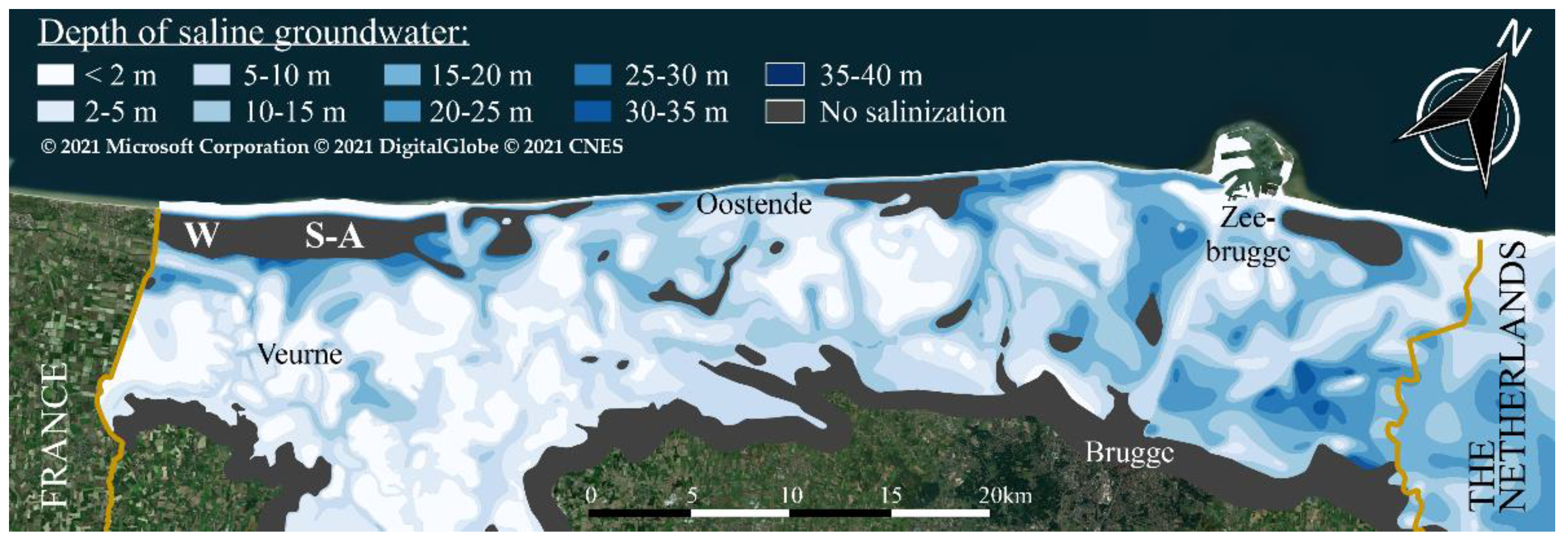
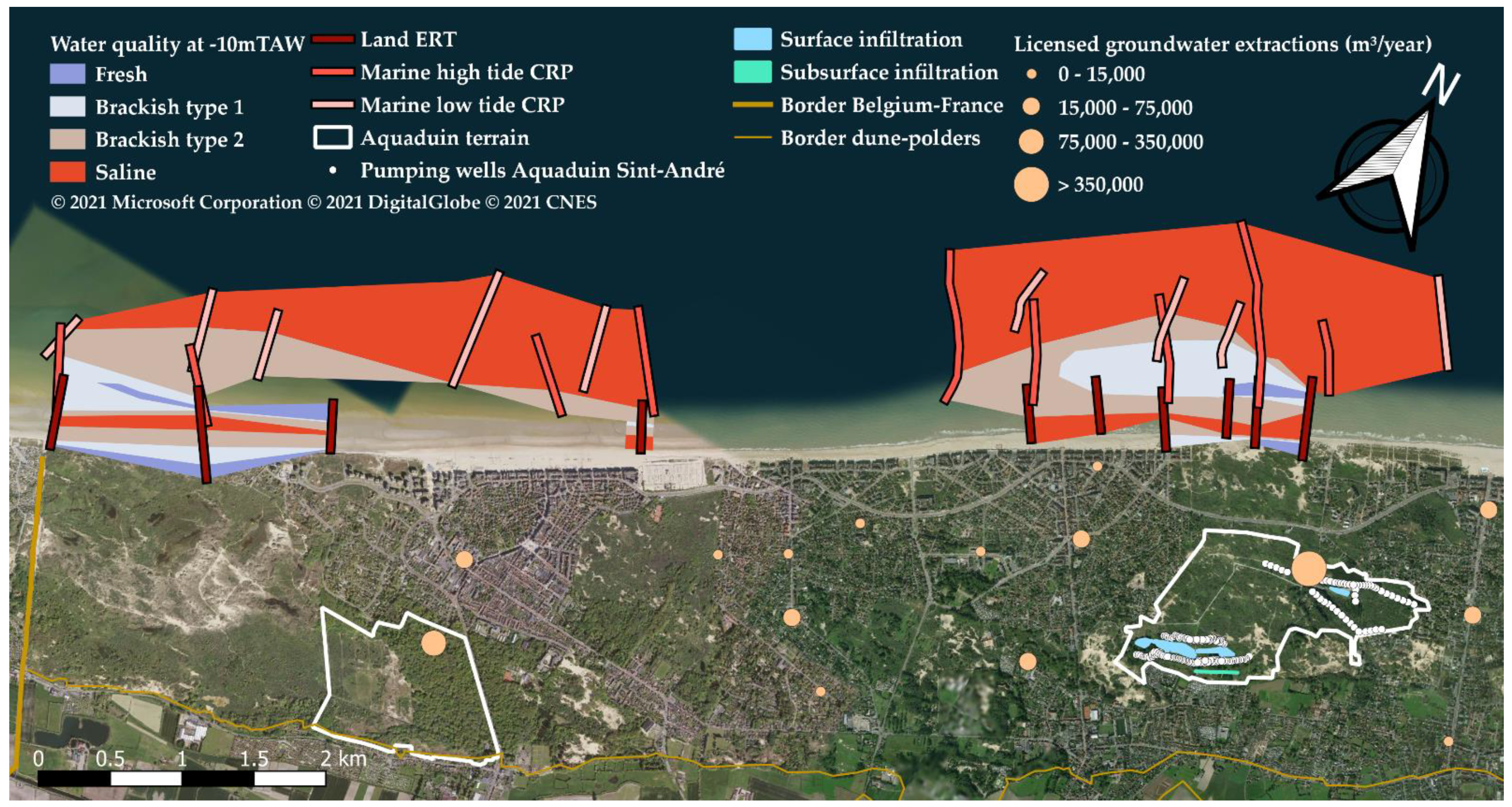
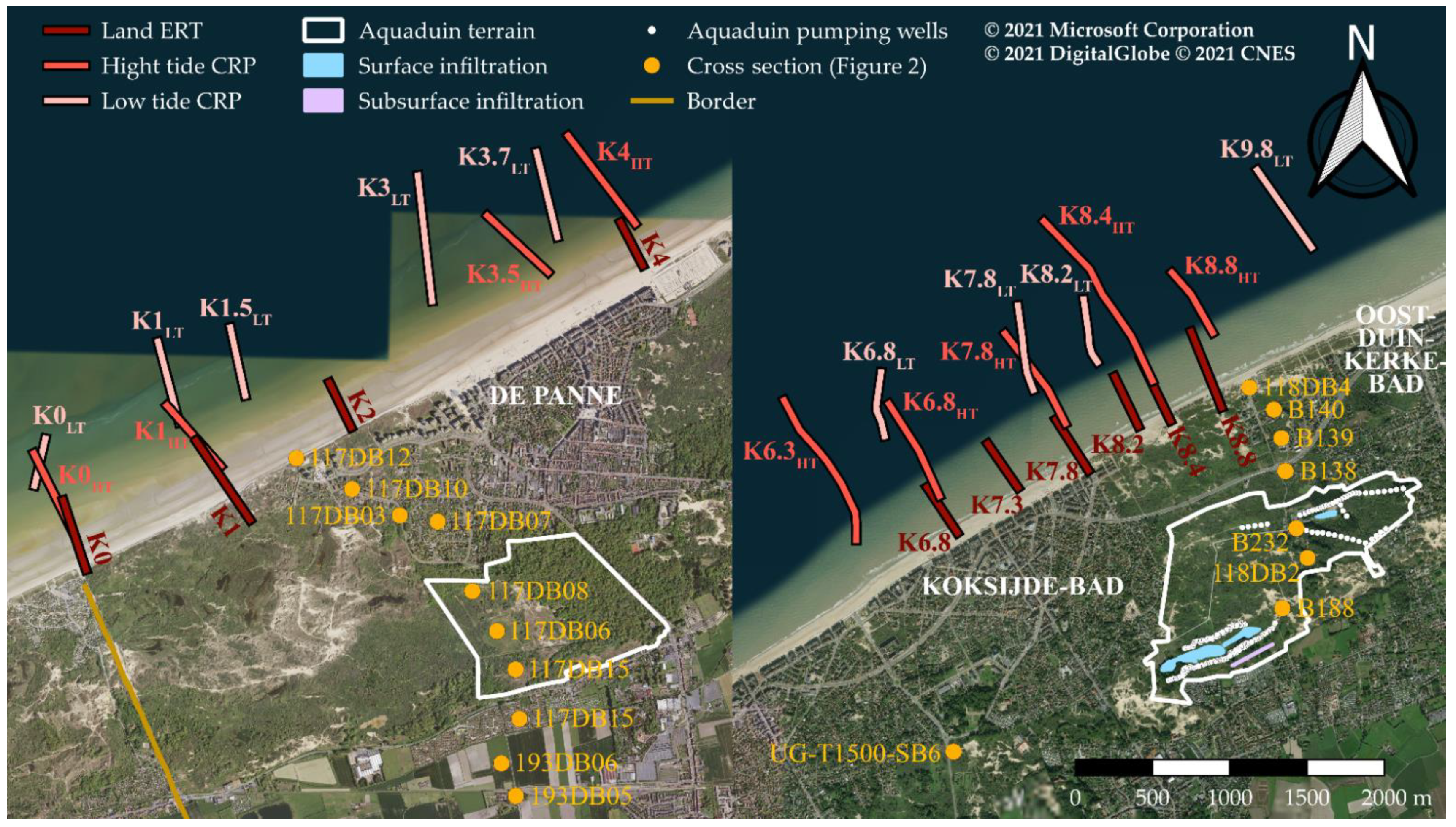
2. Study Area
3. Material and Methods
3.1. Electrical Resistivity Tomography
3.2. Continuous Resistivity Profiling
3.3. Inversion and Interpretation
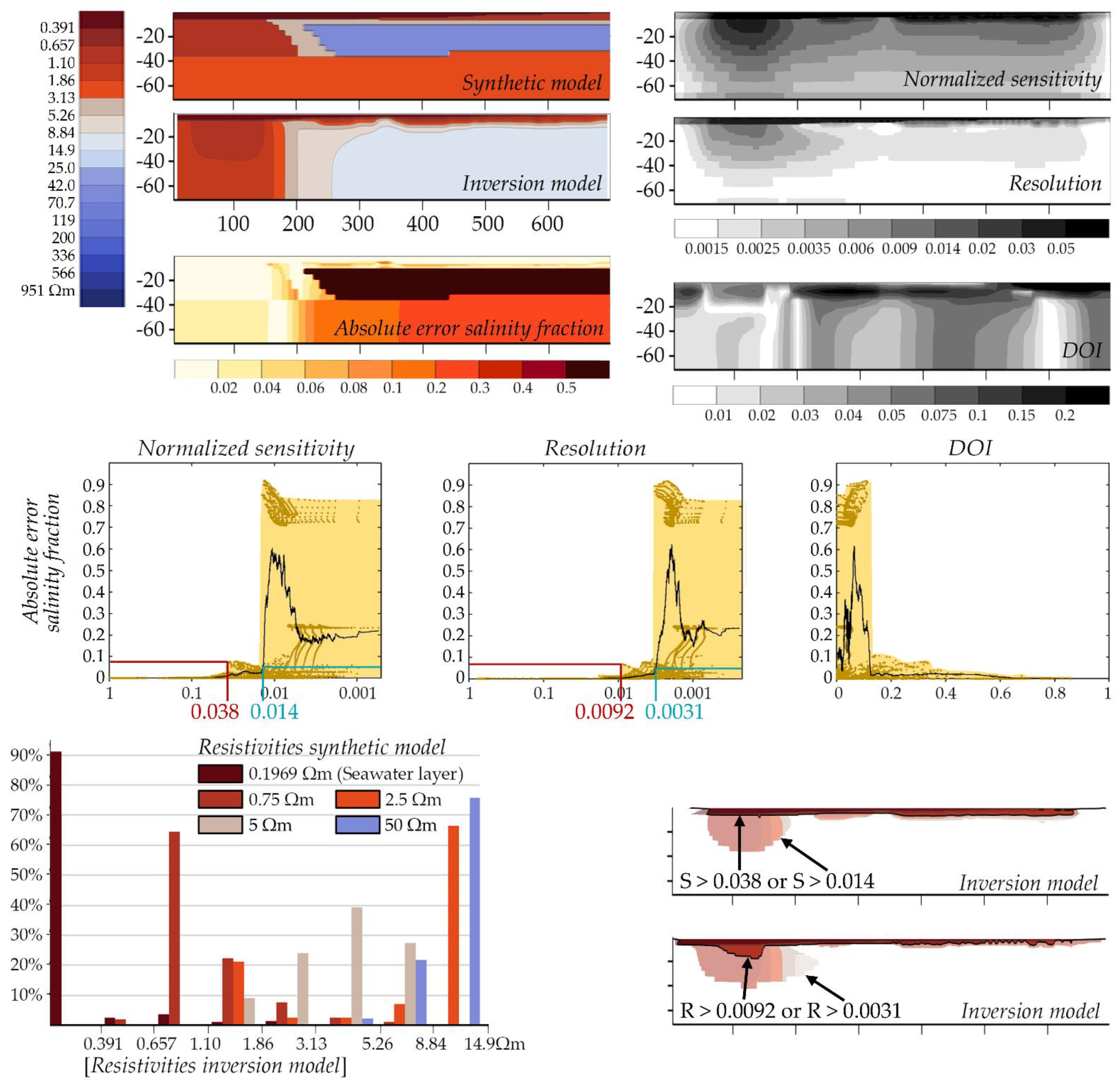
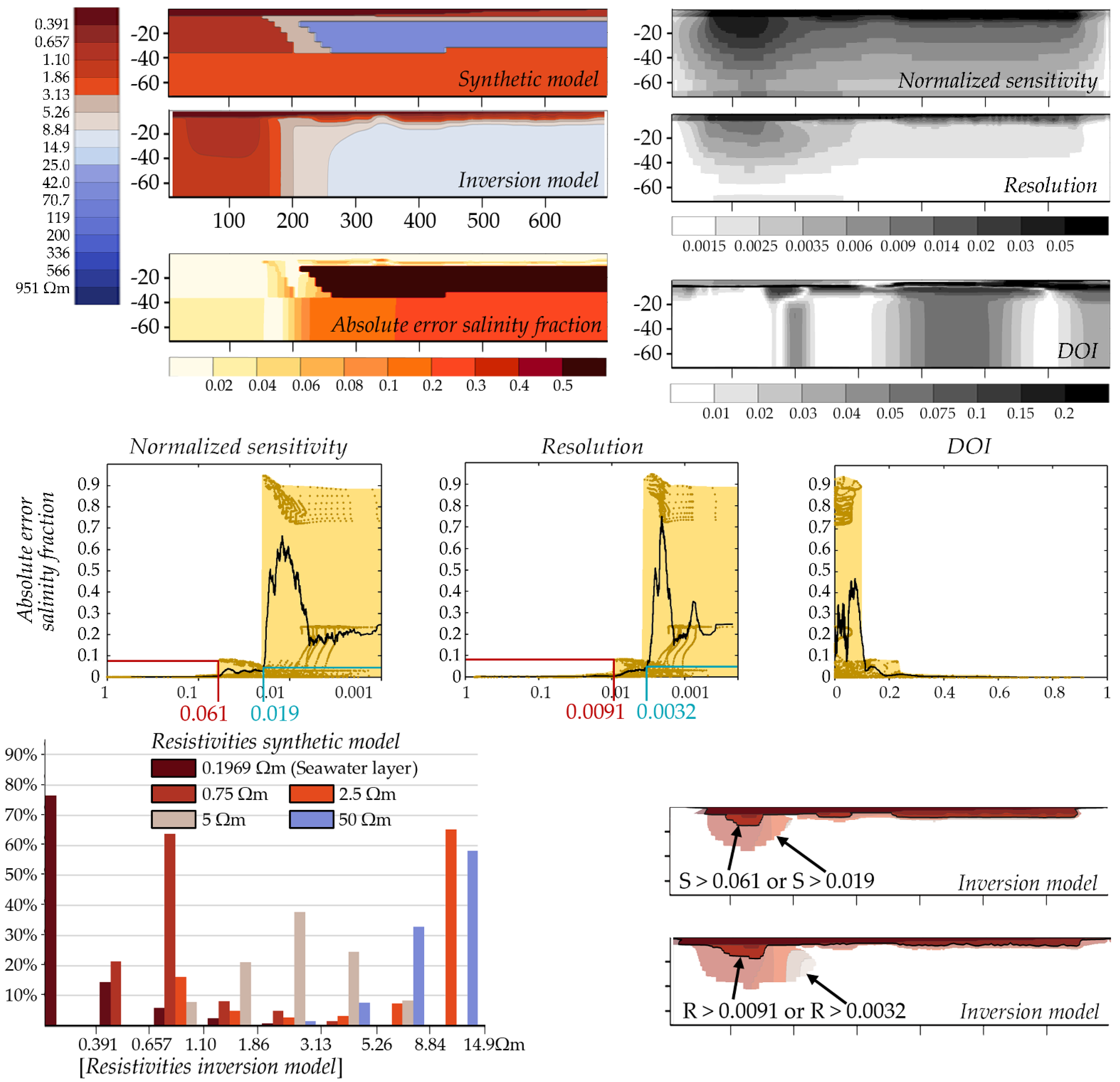
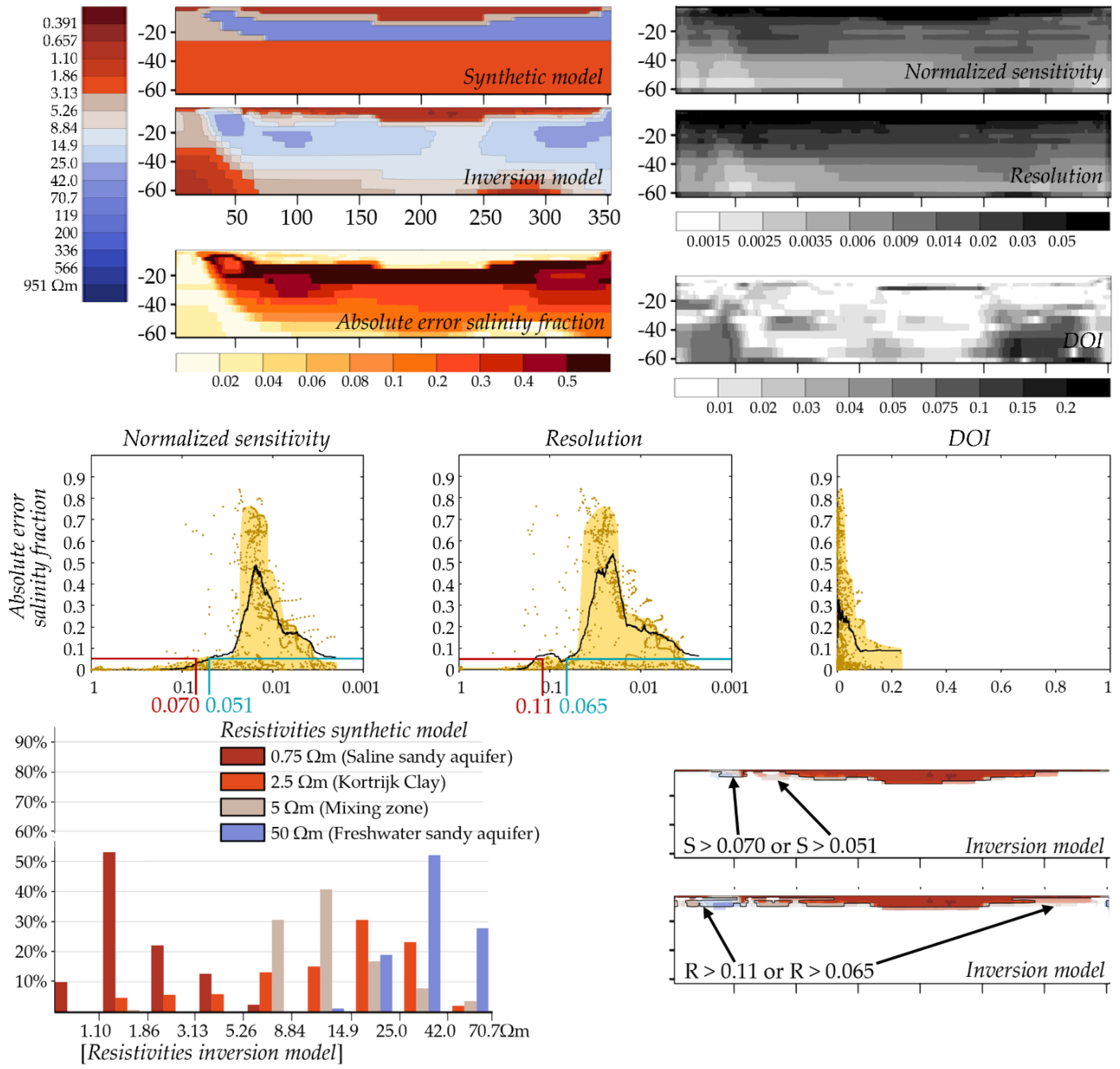
3.4. Image Appraisal Tools
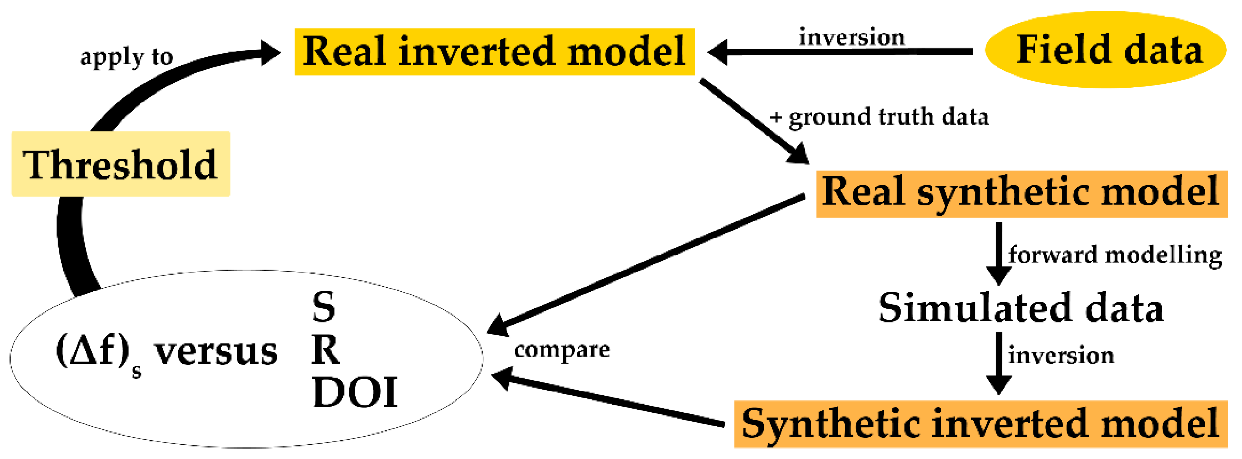
- (1)
- Field data is acquired for which a real inverted model is obtained.
- (2)
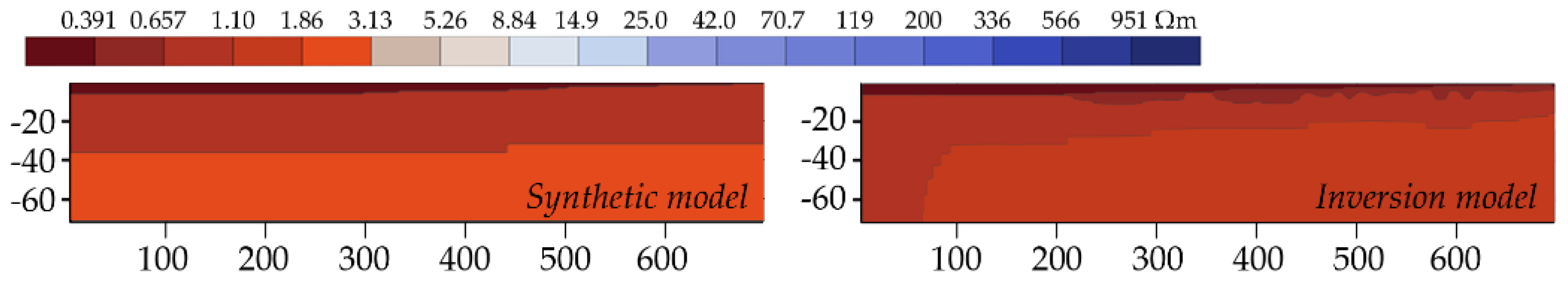
- A real synthetic model is defined, which resembles the real inverted model and includes known ground truth data.
- (3)
- After forward modelling of this model, the simulated data is inverted to obtain a synthetic inverted model. The same inversion parameters (electrode array, inversion parameters, etc.) are used as for the field data, and the DOI, R, and S are calculated (see Section 3.4.1–Section 3.4.3).
- (4)
- The real synthetic model and the synthetic inverted model are compared, allowing the evaluation of the absolute error on the salinity fraction (, between 0 and 1), which is used to define the bulk resistivity ():for which we used 0.1969 Ωm as the bulk saltwater resistivity () and 50 Ωm to represent the bulk freshwater resistivity ().
- (5)
- The error is evaluated against the DOI, R, and S to define a threshold.
- (9)
- The thresholds can be applied to the real inverted model.
3.4.1. Depth of Investigation (DOI)
3.4.2. Model Resolution
3.4.3. Cumulative Sensitivity
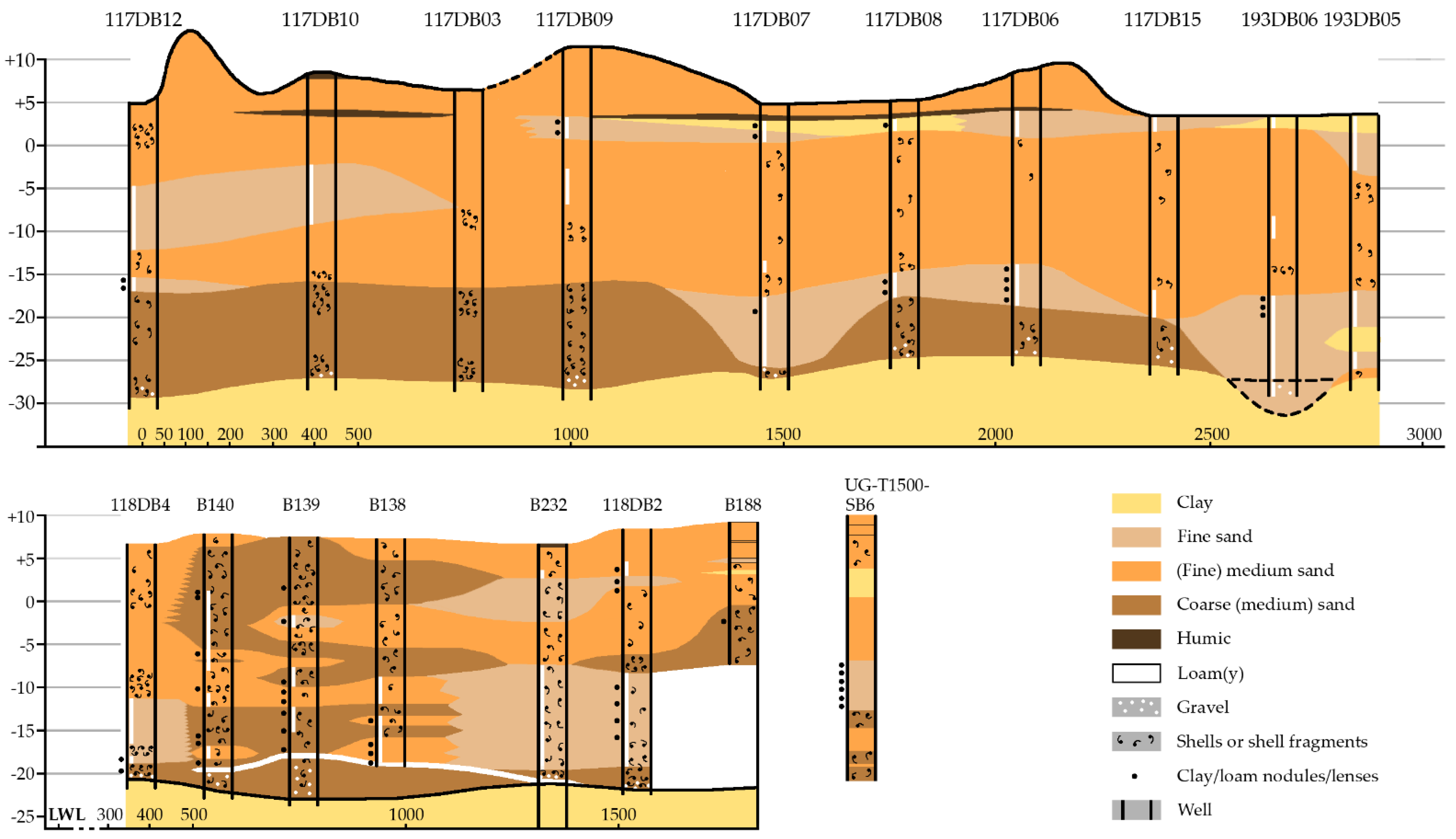
3.5. Existing Groundwater Models of the Area
4. Results
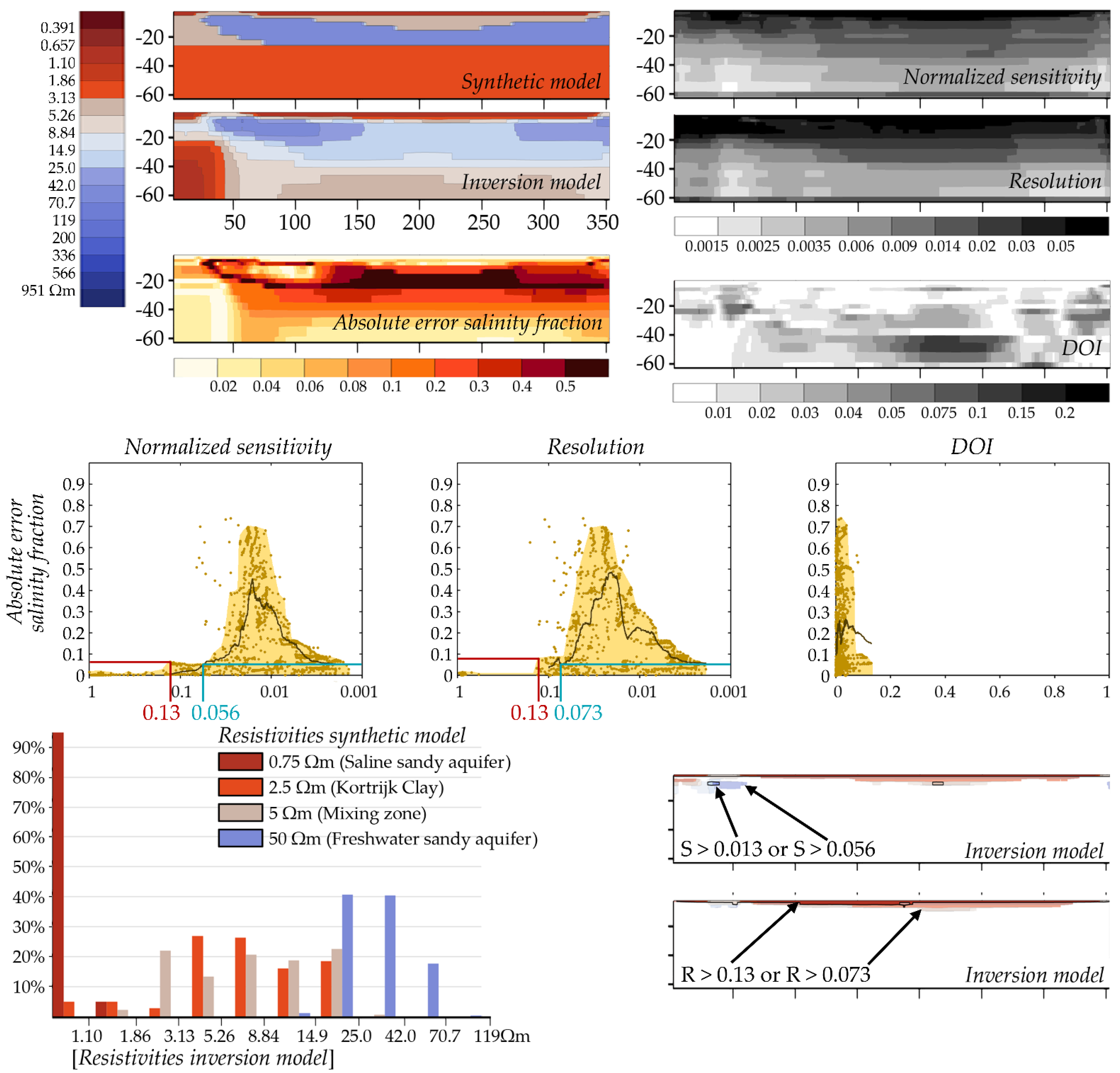
4.1. Synthetic Models
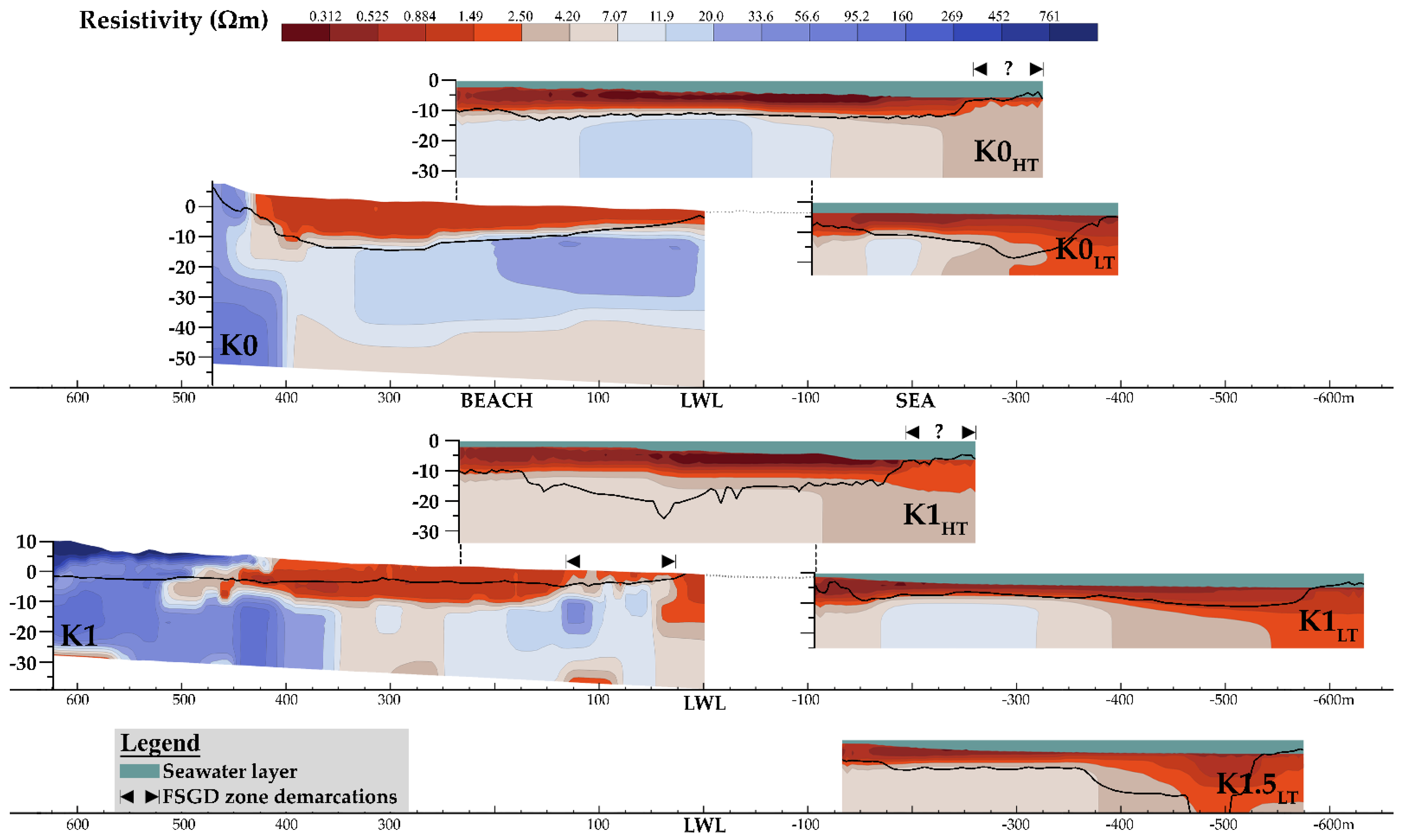
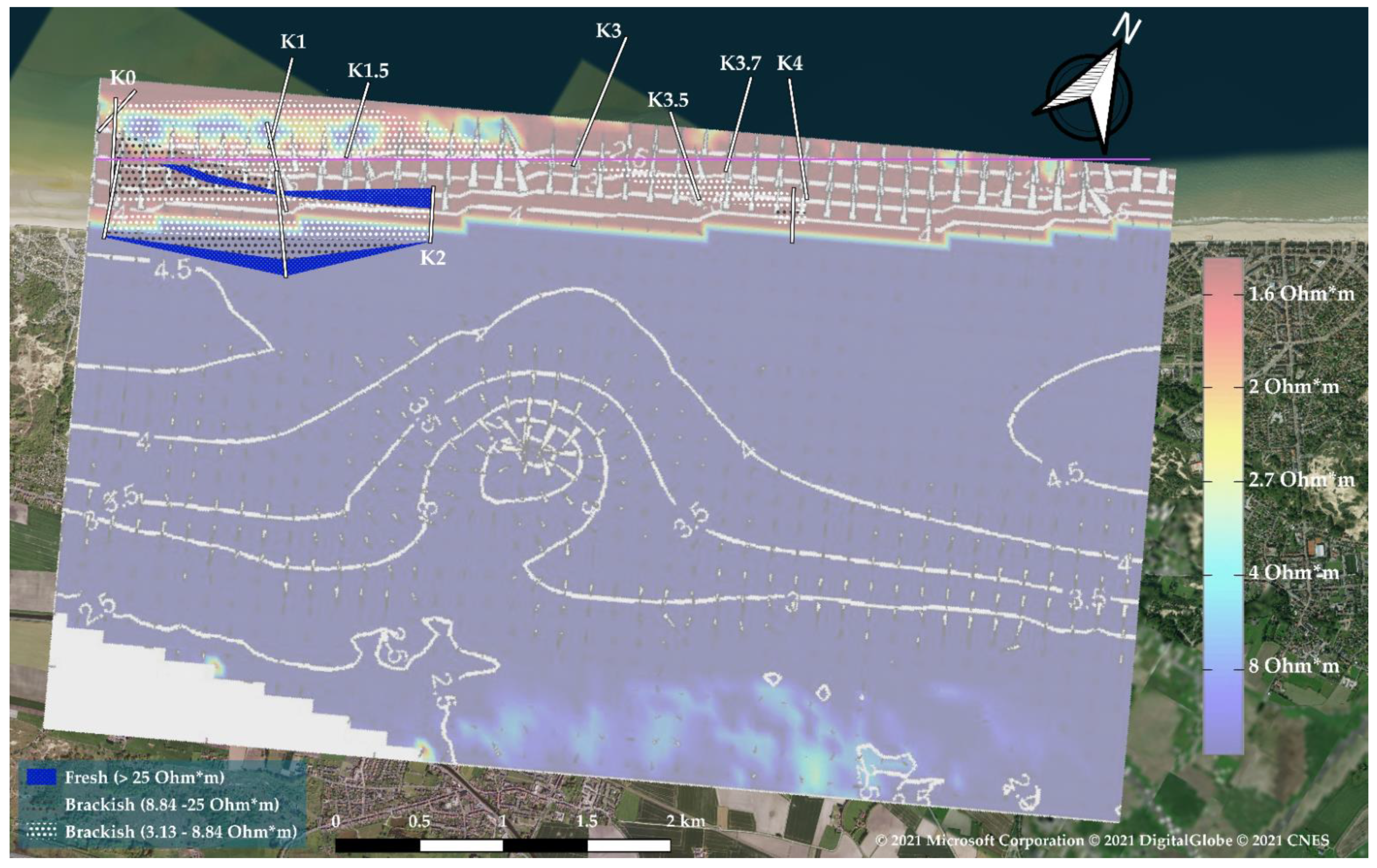
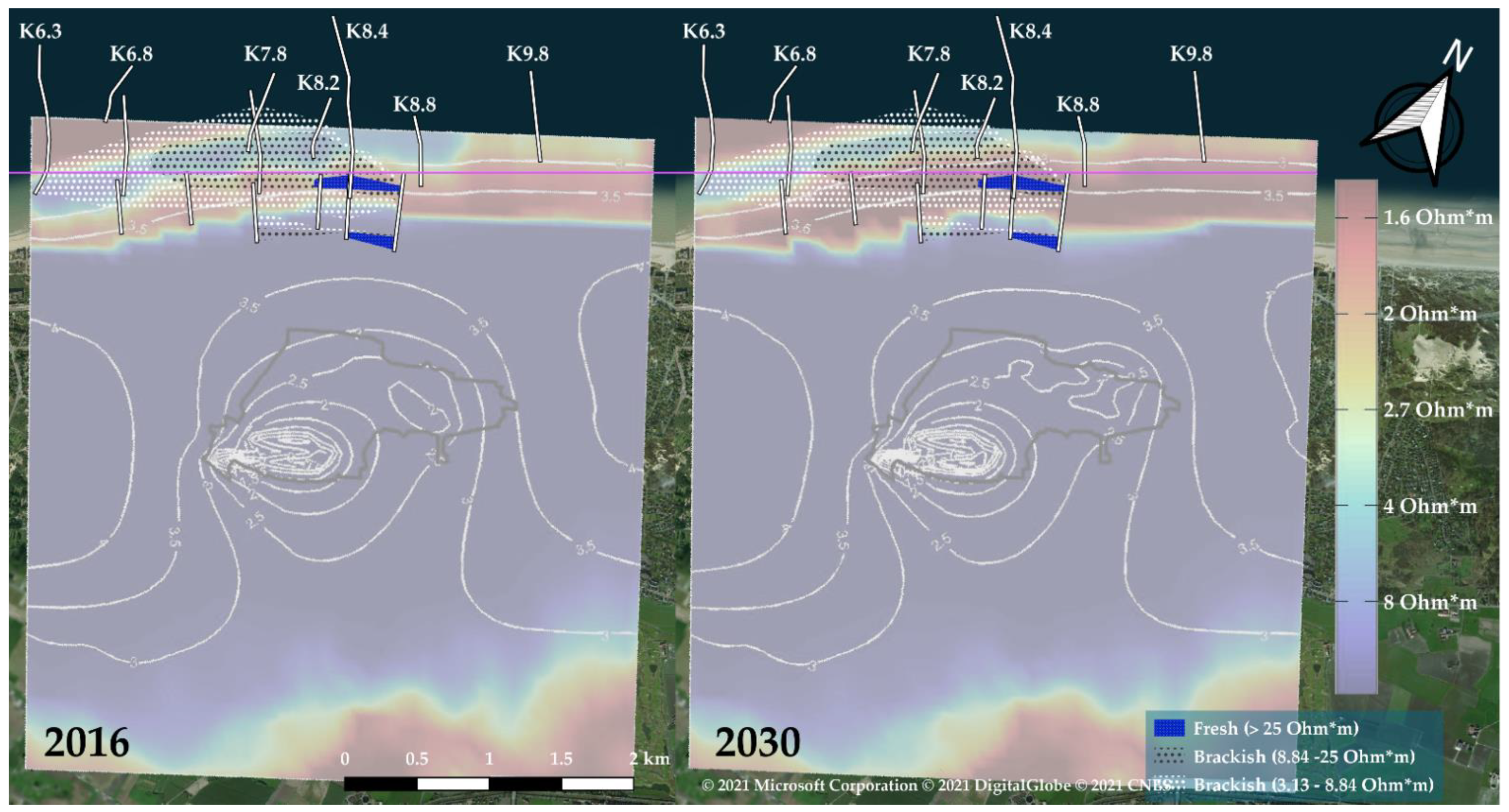
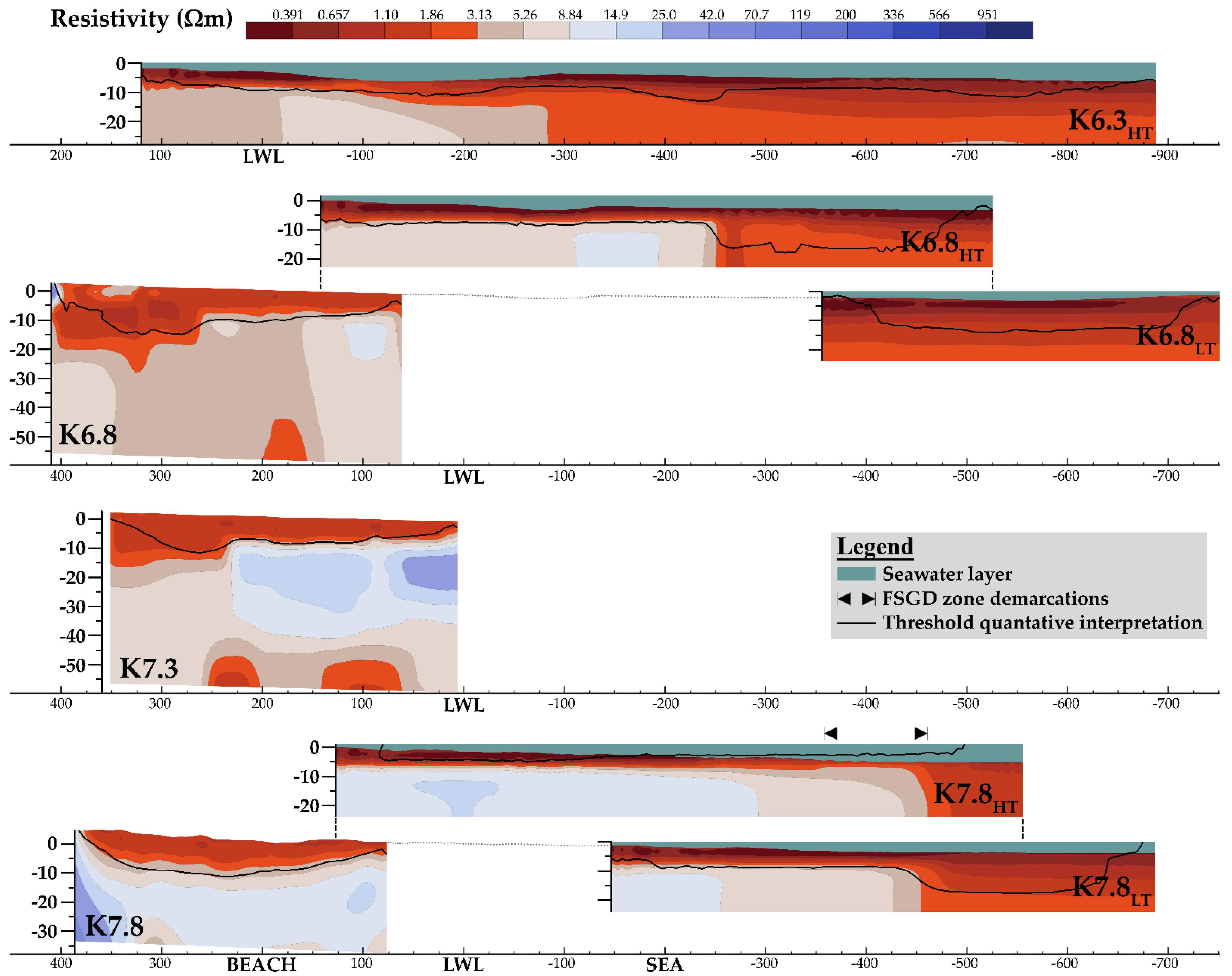
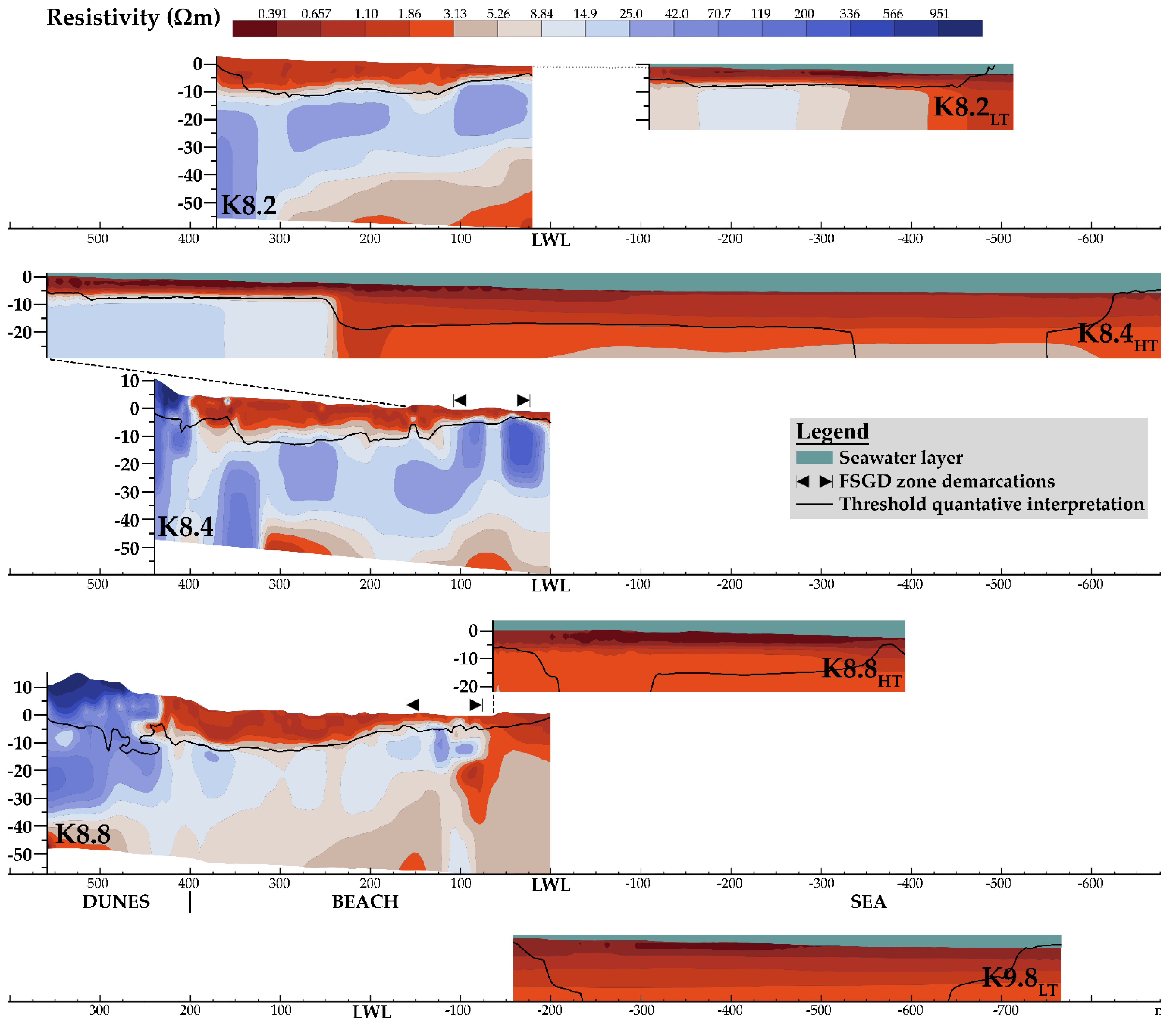
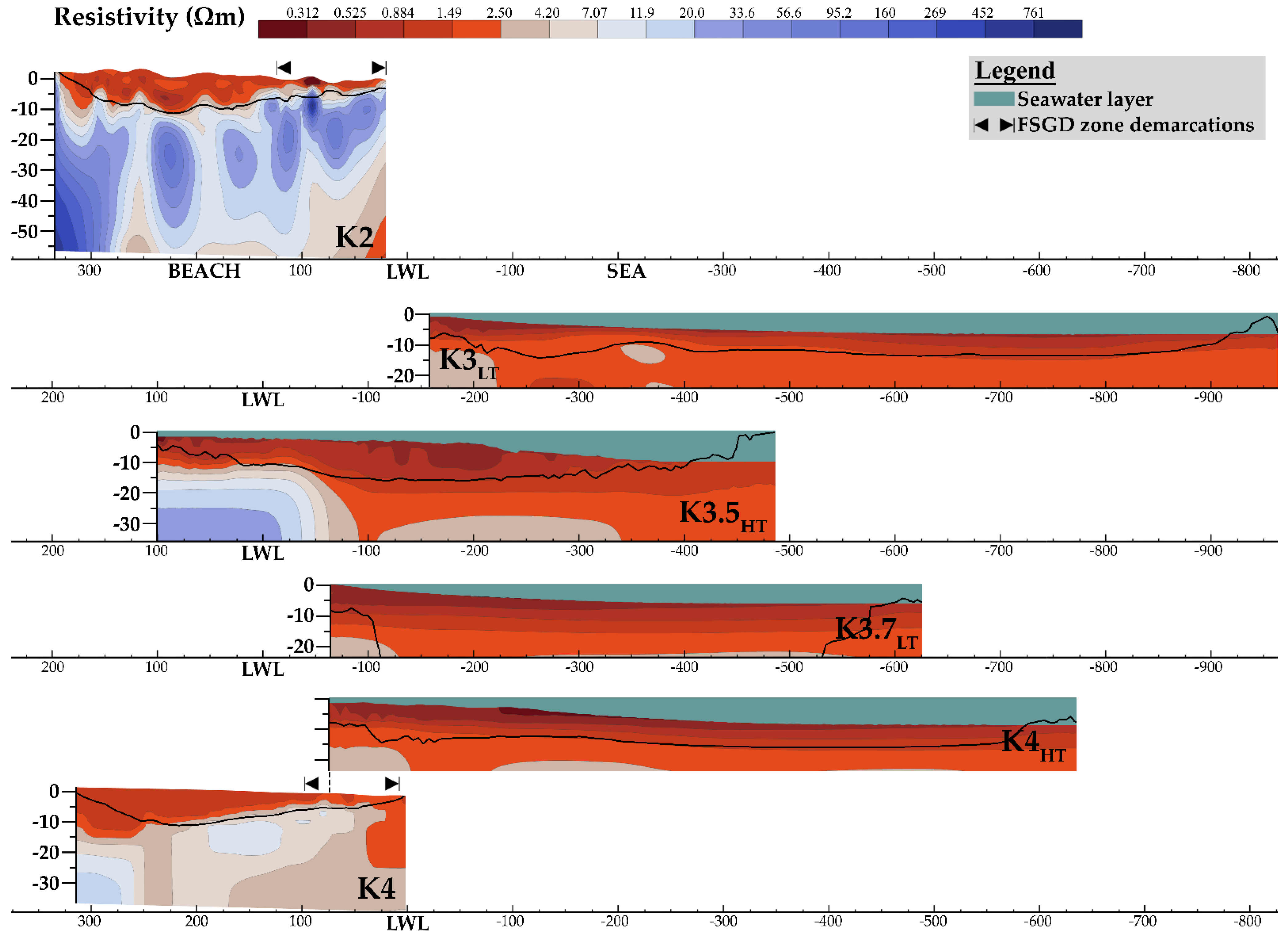
4.2. Field Data
5. Discussion
5.1. Anthropogenic Effects on FSGD
5.2. Comparison with Existing Groundwater Models: De Westhoek
5.3. Comparison with Existing Groundwater Models: Sint-André
6. Conclusions
Author Contributions
Funding
Data Availability Statement
Acknowledgments
Conflicts of Interest
References
- Luijendijk, E.; Gleeson, T.; Moosdorf, N. Fresh groundwater discharge insignificant for the world’s oceans but important for coastal ecosystems. Nat. Commun. 2020, 11, 1260. [Google Scholar] [CrossRef] [PubMed] [Green Version]
- Bratton, J.E. The Three Scales of Submarine Groundwater Flow and Discharge across Passive Continental Margins. J. Geol. 2010, 118, 565–575. [Google Scholar] [CrossRef] [Green Version]
- Moosdorf, N.; Oehler, T. Societal use of fresh submarine groundwater discharge: An overlooked water resource. Earth Sci. Rev. 2017, 171, 338–348. [Google Scholar] [CrossRef]
- Santos, I.R.; Chen, X.; Lecher, A.L.; Sawyer, A.H.; Moosdorf, N.; Rodellas, V.; Tamborski, J.; Cho, H.-M.; Dimova, N.; Sugimoto, R.; et al. Submarine groundwater discharge impacts on coastal nutrient biogeochemistry. Nat. Rev. Earth Environ. 2021, 2, 307–323. [Google Scholar] [CrossRef]
- Zamani, M.G.; Moridi, A.; Yazdi, J. Groundwater management in arid and semi-arid regions. Arab. J. Geosci. 2022, 15, 362. [Google Scholar] [CrossRef]
- Braga, A.C.R.; Serrao-Neumann, S.; de Oliveira Galvão, C. Groundwater management in coastal areas through landscape scale planning: A systematic literature review. Environ. Manag. 2020, 65, 321–333. [Google Scholar] [CrossRef] [PubMed]
- Masciopinto, C.; Vurro, M.; Palmisano, V.N.; Liso, I.S. A Suitable Tool for Sustainable Groundwater Management. Water Resour. Manag. 2017, 31, 4133–4147. [Google Scholar] [CrossRef]
- Lebbe, L. Grondwatermodel Van De Geplande Wijzigingen in Waterwinning Sint-André; Universiteit Gent: Gent, Belgium, 2017; p. 140. [Google Scholar]
- Werner, A.D.; Bakker, M.; Post, V.A.E.; Vandenbohede, A.; Lu, C.; Ataie-Ashtiani, B.; Simmons, C.T.; Barry, D.A. Seawater intrusion processes, investigation and management: Recent advances and future challenges. Adv. Water Resour. 2013, 51, 3–26. [Google Scholar] [CrossRef]
- White, E.; Kaplan, D. Restore or retreat? Saltwater intrusion and water management in coastal wetlands. Ecosyst. Health Sustain. 2017, 3, e01258. [Google Scholar] [CrossRef] [Green Version]
- Van Houtte, E.; Verbauwhede, J. Environmental benefits from water reuse combined with managed aquifer recharge in the Flemish dunes (Belgium). Int. J. Water Resour. Dev. 2021, 37, 1027–1034. [Google Scholar] [CrossRef]
- Bachtouli, S.; Comte, J.-C. Regional-scale analysis of the effect of managed aquifer recharge on saltwater intrusion in irrigated coastal aquifers: Long-term groundwater observations and model simulations in NE Tunisia. J. Coast. Res. 2019, 35, 91–109. [Google Scholar] [CrossRef]
- Dillon, P. Future management aquifer recharge. Hydrogeol. J. 2005, 13, 313–316. [Google Scholar] [CrossRef]
- Vandenbohede, A.; Van Houtte, E.; Lebbe, L. Sustainable groundwater extraction in coastal areas: A Belgian example. Environ. Geol. 2008, 57, 735–747. [Google Scholar] [CrossRef]
- Paepen, M.; Hanssens, D.; De Smedt, P.; Walraevens, K.; Hermans, T. Combining resistivity and frequency domain electromagnetic methods to investigate submarine groundwater discharge (SGD) in the littoral zone. Hydrol. Earth Syst. Sci. 2020, 24, 3539–3555. [Google Scholar] [CrossRef]
- Cantarero, D.L.M.; Blanco, A.; Cardenas, M.B.; Nadaoka, K.; Siringan, F.P. Offshore Submarine Groundwater Discharge at a Coral Reef Front Controlled by Faults. Geochem. Geophys. Geosystems. 2019, 20, 8310. [Google Scholar] [CrossRef]
- Goebel, M.; Pidlisecky, A.; Knight, R. Resistivity imaging reveals complex pattern of saltwater intrusion along Monterey coast. J. Hydrol. 2017, 551, 746–755. [Google Scholar] [CrossRef]
- Cong-Thi, D.; Pham Dieu, L.; Thibaut, R.; Paepen, M.; Hieu Ho, H.; Nguyen, F.; Hermans, T. Imaging the Structure and the Saltwater Intrusion Extent of the Luy River Coastal Aquifer (Binh Thuan, Vietnam) Using Electrical Resistivity Tomography. Water 2021, 13, 1743. [Google Scholar] [CrossRef]
- González-Quirós, A.; Comte, J.-C. Relative importance of conceptual and computational errors when delineating saltwater intrusion from resistivity inverse models in heterogeneous coastal aquifers. Adv. Water Resour. 2020, 144, 103695. [Google Scholar] [CrossRef]
- Day-Lewis, F.D.; Singha, K.; Binley, A.M. Applying petrophysical models to radar travel time and electrical resistivity tomograms: Resolution-dependent limitations. J. Geophys. Res. 2005, 110, 3569. [Google Scholar] [CrossRef] [Green Version]
- Binley, A.; Kemna, A. DC Resistivity and Induced Polarization Methods. In Hydrogeophyscis; Rubin, Y., Hubbard, S.S., Eds.; Springer: Dordrecht, The Netherlands, 2005; Volume 50. [Google Scholar]
- Caterina, D.; Beaujean, J.; Tanguy, R.; Nguyen, F. A comparison study of different image appraisal tools for electrical resistivity tomography. Near Surf. Geophys. 2013, 11, 639–657. [Google Scholar] [CrossRef]
- Wilson, S.R.; Ingham, M.; McConchie, J.A. The applicability of earth resistivity methods for saline interface definition. J. Hydrol. 2006, 316, 301–312. [Google Scholar] [CrossRef]
- Comte, J.-C.; Banton, O. Cross-validation of geo-electrical and hydrogeological models to evaluate seawater intrusion in coastal aquifers. Geophys. Res. Lett. 2007, 34, L10402. [Google Scholar] [CrossRef]
- Nguyen, F.; Kemna, A.; Antonsson, A.; Engesgaard, P.; Kuras, O.; Ogilvy, R.; Gisbert, J.; Jorreto, S.; Pulido-Bosch, A. Characterization of seawater intrusion using 2D electrical imaging. Near Surf. Geophys. 2009, 7, 377–390. [Google Scholar] [CrossRef] [Green Version]
- Beaujean, J.; Nguyen, F.; Kemna, A.; Engensgaard, P. Joint and sequential inversion of geophysical and hydrogeological data to characterize seawater intrusion models. In Proceedings of the 21st Salt Water Intrusion Meeting, Ponta Delgada, Portugal, 21–25 June 2010; pp. 57–60. [Google Scholar]
- Hermans, T.; Vandenbohede, A.; Lebbe, L.; Martin, R.; Kemna, A.; Beaujean, J.; Nguyen, F. Imaging artificial salt water infiltration using electrical resistivity tomography constrained by geostatistical data. J. Hydrol. 2012, 438–439, 168–180. [Google Scholar] [CrossRef] [Green Version]
- Zeynolabedin, A.; Ghiassi, R.; Norooz, R.; Najib, S.; Fadili, A. Evaluation of geoelectrical models efficiency for coastal seawater intrusion by applying uncertainty analysis. J. Hydol. 2021, 603, 127086. [Google Scholar] [CrossRef]
- Taniguchi, M.; Dulai, H.; Burnett, K.M.; Santos, I.R.; Sugimoto, R.; Stieglitz, T.; Kim, G.; Moosdorf, N.; Burnett, W.C. Submarine Groundwater Discharge: Updates on Its Measurement Techniques, Geophysical Drivers, Magnitudes, and Effects. Front. Environ. Sci. 2019, 7, 141. [Google Scholar] [CrossRef]
- Vandenbohede, A.; Lebbe, L. De Panne—Natuurreservaat—De Westhoek Monitoring Grondwater Slufters. Fase 2; Universiteit Gent: Gent, Belgium, 2008. [Google Scholar]
- Baeteman, C. The Holocene depositional history of the IJzer palaeovalley (Western Belgian coastal plain) with reference to the factors controlling the formation of intercalated peat beds. Geol. Belg. 1999, 2, 39–72. [Google Scholar] [CrossRef]
- Van Meir, N.; Lebbe, L. Simulations of Evolution of Salt-Water Distribution in Young Dunes near the French-Belgian Border. Nat. Tijdschr. 1997, 79, 105–113. [Google Scholar]
- Baeteman, C. Chronology of coastal plain development during the Holocene in West Belgium. Quaternaire 1991, 2, 116–125. [Google Scholar] [CrossRef]
- De Breuck, W.; De Moor, G.; Maréchal, R.; Tavernier, R. Diepte van het grensvlak tussen zoet en zout water in de freatisch laag van het Belgische kustgebied (1963–1973). In Verziltingskaart; Militair Geografisch Instituut: Brussel, Belgium, 1974. [Google Scholar]
- Vandenbohede, A.; Van Houtte, E.; Lebbe, L. Water quality changes in the dunes of the western Belgian coastal plain due to artificial recharge of tertiary treated wastewater. Appl. Geochem. 2009, 24, 370–382. [Google Scholar] [CrossRef]
- Vandenbohede, A.; Lebbe, L. Occurrence of salt water above fresh water in dynamic equilibrium in a coastal groundwater flow system near De Panne, Belgium. Hydrogeol. J. 2006, 14, 462–472. [Google Scholar] [CrossRef]
- Vandenbohede, A.; Van Houtte, E.; Lebbe, L. Groundwater flow in the vicinity of two artificial recharge ponds in the Belgian coastal dunes. Hydrogeol. J. 2008, 16, 1669–1681. [Google Scholar] [CrossRef]
- Lebbe, L.; De Breuck, W. Hydrogeologie van het duingebied tussen Koksijde en Oostduinkerke. Tijdschr. Van Het Belg. Cent. Voor De Stud. Van Water Bodem En Lucht 1980, 55, 33–45. [Google Scholar]
- Lebbe, L. Hydrogeologie van het duingebied ten westen van De Panne. In Docoraatsverhandeling; Rijksuniversiteit Gent: Gent, Belgium, 1978. [Google Scholar]
- Lebbe, L. Litostratigrafie en hydraulische doorlatendheid van het freatische reservoir te De Panne. Nat. Tijdschr. 1979, 61, 29–58. [Google Scholar]
- Van Houtte, E.; Verbauwhede, J. Switching Between Open And Subsurface Infiltration According To Temperature. In Proceedings of the 48th IAH Congress, Brussels, Belgium, 6–10 September 2021; pp. 103–104. [Google Scholar]
- IWVA. Jaarverslag 2019; IWVA: Koksijde, Belgium, 2019; p. 58. [Google Scholar]
- Martens, K.; Walraevens, K.; Lebbe, L. Ecosysteemvisie Voor De Vlaamse Kust—Deelstudie: Hydrogeologie Synthese; Universiteit Gent—Toegepaste Geologie en Hydrogeologie: Gent, Belgium, 1995. [Google Scholar]
- Lebbe, L. Parameter identifcation in fresh-saltwater flow based on borehole resistivities and freshwater head data. Adv. Water Resour. 1999, 22, 791–806. [Google Scholar] [CrossRef]
- Vandenbohede, A.; Lebbe, L.; Gysens, S.; Delecluyse, K.; Dewolf, P. Salt water infiltration in two artificial sea inlets in the Belgian dune area. J. Hydrol. 2008, 360, 77–86. [Google Scholar] [CrossRef]
- Dahlin, T.; Zhou, B. Multiple-gradient array measurements for multichannel 2D resistivity imaging. Near Surf. Geophys. 2006, 4, 113–123. [Google Scholar] [CrossRef] [Green Version]
- Loke, M.H. Rapid 2-D Resistivity & IP Inversion Using the Least-Squares Method; Geotomo Software: Penang, Malaysia, 2011; p. 152. [Google Scholar]
- De Breuck, W.; De Moor, G. The water-table aquifer in the Eastern coastal area of Belgium. Hydrol. Sci. J. 1969, 14, 137–155. [Google Scholar] [CrossRef]
- Oldenburg, D.W.; Li, Y. Estimating depth of investigation in dc resistivity and IP surveys. Geophysics 1999, 64, 403–416. [Google Scholar] [CrossRef]
- Kemna, A. Tomographic Inversion of Complex Resistivity: Theory and Application; Ruhr-Universität Bochum: Osnabrück, Germany, 2000. [Google Scholar]
- Lebbe, L. The subterranean flow of fresh and salt water underneath the Western Belgian beach. In Proceedings of the 7th Salt Water Intrusion Meeting, Uppsala, Sweden, 14–17 September 1981; pp. 193–219. [Google Scholar]
- IWVA. Jaarrapport 2005; IWVA: Koksijde, Belgium, 2005; p. 47. [Google Scholar]


| Name | Length (m) | Array Type | Electrode Spacing (m) | Date | Figure | Reference |
|---|---|---|---|---|---|---|
| K0 | 475 | Multiple-gradient | 5 | 11 October 2018 | 11 | [15] |
| K0HT | 586 | Reciprocal Wenner–Schlumberger | 15 | 30 May 2018 | 11 | [15] |
| K0LT | 297 | Reciprocal Wenner–Schlumberger | 10 | 22 May 2019 | 11 | [15] |
| K1 | 625 | Multiple-gradient | 5 | 7 March 2018 | 11 | [15] |
| K1HT | 517 | Reciprocal Wenner–Schlumberger | 15 | 30 May 2018 | 11 | [15] |
| K1LT | 537 | Reciprocal Wenner–Schlumberger | 10 | 22 May 2019 | 11 | [15] |
| K1.5LT | 449 | Reciprocal Wenner–Schlumberger | 10 | 22 May 2019 | 11 | [15] |
| K2 | 320 | Multiple-gradient | 5 | 6 October 2020 | 12 | - |
| K3LT | 819 | Reciprocal Wenner–Schlumberger | 10 | 22 May 2019 | 12 | - |
| K3.5HT | 586 | Reciprocal Wenner–Schlumberger | 15 | 30 May 2018 | 12 | - |
| K3.7LT | 566 | Reciprocal Wenner–Schlumberger | 10 | 22 May 2019 | 12 | - |
| K4 | 315 | Multiple-gradient | 5 | 12 October 2018 | 12 | |
| K4HT | 717 | Reciprocal Wenner–Schlumberger | 10 | 29 May 2019 | 12 | - |
| K6.3HT | 1023 | Reciprocal Wenner–Schlumberger | 10 | 29 May 2019 | 9 | - |
| K6.8 | 360 | Multiple-gradient | 5 | 19 March 2021 | 9 | - |
| K6.8HT | 699 | Reciprocal Wenner–Schlumberger | 10 | 29 May 2019 | 9 | - |
| K6.8LT | 419 | Reciprocal Wenner–Schlumberger | 10 | 22 May 2019 | 9 | - |
| K9.3 | 360 | Multiple-gradient | 5 | 16 March 2021 | 9 | - |
| K9.8 | 320 | Multiple-gradient | 5 | 25 June 2019 | 9 | - |
| K9.8HT | 693 | Reciprocal Wenner–Schlumberger | 10 | 29 May 2019 | 9 | - |
| K9.8LT | 549 | Reciprocal Wenner–Schlumberger | 10 | 22 May 2019 | 9 | - |
| K8.2 | 360 | Multiple-gradient | 5 | 19 March 2021 | 10 | - |
| K8.2LT | 410 | Reciprocal Wenner–Schlumberger | 10 | 22 May 2019 | 10 | - |
| K8.4 | 450 | Multiple-gradient | 5 | 22 September 2020 | 10 | - |
| K8.4HT | 1254 | Reciprocal Wenner–Schlumberger | 10 | 29 May 2019 | 10 | - |
| K8.8 | 540 | Multiple-gradient | 5 | 21 September 2020 | 10 | - |
| K8.8HT | 494 | Reciprocal Wenner–Schlumberger | 10 | 29 May 2019 | 10 | - |
| K9.8LT | 615 | Reciprocal Wenner–Schlumberger | 10 | 22 May 2019 | 10 | - |
Publisher’s Note: MDPI stays neutral with regard to jurisdictional claims in published maps and institutional affiliations. |
© 2022 by the authors. Licensee MDPI, Basel, Switzerland. This article is an open access article distributed under the terms and conditions of the Creative Commons Attribution (CC BY) license (https://creativecommons.org/licenses/by/4.0/).
Share and Cite
Paepen, M.; Deleersnyder, W.; De Latte, S.; Walraevens, K.; Hermans, T. Effect of Groundwater Extraction and Artificial Recharge on the Geophysical Footprints of Fresh Submarine Groundwater Discharge in the Western Belgian Coastal Area. Water 2022, 14, 1040. https://doi.org/10.3390/w14071040
Paepen M, Deleersnyder W, De Latte S, Walraevens K, Hermans T. Effect of Groundwater Extraction and Artificial Recharge on the Geophysical Footprints of Fresh Submarine Groundwater Discharge in the Western Belgian Coastal Area. Water. 2022; 14(7):1040. https://doi.org/10.3390/w14071040
Chicago/Turabian StylePaepen, Marieke, Wouter Deleersnyder, Sybren De Latte, Kristine Walraevens, and Thomas Hermans. 2022. "Effect of Groundwater Extraction and Artificial Recharge on the Geophysical Footprints of Fresh Submarine Groundwater Discharge in the Western Belgian Coastal Area" Water 14, no. 7: 1040. https://doi.org/10.3390/w14071040
APA StylePaepen, M., Deleersnyder, W., De Latte, S., Walraevens, K., & Hermans, T. (2022). Effect of Groundwater Extraction and Artificial Recharge on the Geophysical Footprints of Fresh Submarine Groundwater Discharge in the Western Belgian Coastal Area. Water, 14(7), 1040. https://doi.org/10.3390/w14071040