Development and Evaluation of a Saturated Zone Module in an Integrated Urban Hydrological Model

Abstract

Shallow urban groundwater interacts with surface water and underground infrastructures. Low-impact development in urban water management by at-source infiltration should consider shallow urban groundwater in a holistic manner. Traditional hydrological models, however, rarely detail groundwater flows and their interaction with urban runoff and the water budget. In the present study, a new approach is proposed, using the integration of a flow module WTI for the saturated zone in a distributed urban hydrological model URBS-MO. This integration is carried out by paying attention to retaining the initial waterflow subsurface parameterization. The performance of the integrated model is evaluated by piezometric and runoff data in an experimental urban catchment, through a sensitivity analysis and a manual calibration of the main model parameters, as well as a validation step. The new module shows its capacity to improve groundwater flow simulation by assessing more realistic water table variations, along with a very small improvement of flowrate simulation. The bias on the average groundwater level was reduced from +14 to +7% for the one-year validation period. The modelling results show the importance of parameter calibration for distributed physically-based hydrological models. Difficulties in the calibration of parameter values due to spatial heterogeneities are also revealed, as the use of piezometric data for the calibration of a hydrological model is rather innovative.

1. Introduction

Urban water is a complex system combining natural water compartments and artificial infrastructures, particularly water supply and sewer systems that modify the natural water cycle. Water flows in the unsaturated and saturated soil layers interact actively with the other compartments. The assessment of the catchment water balance by quantifying these interactions has been the subject of intense studies, but remains one major challenge in urban hydrology [1]. Moreover, low-impact development (LID) practices are being developed worldwide as a way to mitigate the effects of urbanization by preserving pre-development hydrology [2]. Any LID practice for stormwater runoff mitigation can be really efficient only if it does not come into conflict with the equilibrium of the water balance. Moreover, given that most of these LID are infiltration-based, they may significantly affect the groundwater recharge and the base flow [3,4], even though the relation between stormwater infiltration facility insertion and groundwater elevation modification is not straightforward [5].

The urban water system has particularities that distinguish it from natural hydrology, namely reduced temporal and spatial scales, high spatial heterogeneities on the surface and sub-surface, severe impact by human activities, and regular evolutions in land-use, water-use practices and management policies [1]. On the other hand, hydrological processes are not so different in cities and rural areas, and many catchments in the world encompass simultaneously urbanized, natural and agricultural lands [6].

Groundwater can cause insidious problems for underground foundations [3], and underground structures may cause disturbances to the groundwater flow in return [7]. Groundwater is mainly recharged by infiltrated rainfall, but urbanization effects on the water table are variable [8]; irrigation and leakage from pipe infrastructures are other potentially significant contributions to groundwater recharge. Urbanization modifies this natural recharge process due to soil surface imperviousness, decreasing in turn the infiltration [9,10,11], even though the previously evocated LID strategies favor infiltration through vegetated areas like rain gardens or swales [2,3,4,5], allowing stormwater storage in shallow aquifers. On the other hand, evapotranspiration is reduced both by surface sealing and groundwater drains for water level control, and may offset the infiltration lost [12,13]. Water conducted in supply and sewer systems may leak from these infrastructures and become an artificial source of groundwater recharge [14,15,16]. These urban interactions of surface-, ground- and artificial water compartments are complex in time and space, and still leave many questions open [3,17,18]. Observations based on both groundwater levels and sewer or river flowrates may be helpful in order to better understand the shallow groundwater/surface interactions [19,20], but this study will focus on modelling issues.

Given the complexity of urban water systems and continuously enforced regulations such as the European Water Framework Directive, urban planners have to cope with tricky options when they have to define stormwater management strategies. Hydrological models based on the rainfall-runoff response may provide useful information to planners for their decision-making. Existing modelling softwares describe well the hydrological processes on the surface but rarely represent subsurface flows [21], or represent them in very simplified ways [22]. Physically-based, distributed, continuous models are able to represent the spatial and temporal dynamics of the rainfall-runoff response [1] and interactions between stormwater pipes, soil and groundwater [23]. Scientists are working intensively on physically-based integrated models which are capable of addressing the urban water system in more comprehensive ways, including soil and especially vadose zone processes. URBS-MO (Urban Runoff Branching Structure-MOdel) [24] is one of the clearest examples [21], along with the WEP (Water Energy transfer Processes) model [25].

In addition, coupling existing models to enlarge modelling possibilities is a common practice in hydrology. Dynamic coupling has been successfully implemented in various urban studies to better reproduce interactions between surface runoff and subsurface/groundwater flow processes (Table 1). However, these coupling approaches may have some limitations due to the way in which the hydrological variables are transferred from the groundwater model to the surface model [26], or due to the large amount of data needed [27]. The improvement of the vadose zone’s representation within a groundwater flow model may be another option, as is suggested within the MODFLOW code [28].

Table 1. Coupling of surface hydrological models with groundwater flow models in urban areas.

Coupling Models Approaches	Main Objectives and Functionalities
SWMM-FEFLOW [26]	Evaluation of the LID designs effects on groundwater
SWMM-MODFLOW [29]	Simulation of fine temporal scale interactions between Green infrastructures and groundwater
Mike Urban-Mike SHE [4]	Estimation of the extent of the groundwater rise due to urbanization
WEAP-MODFLOW [27]	Simulation of urbanization and irrigation impacts on the groundwater levels, in a semi-arid periurban catchment

Table 1. Coupling of surface hydrological models with groundwater flow models in urban areas.

Coupling Models Approaches	Main Objectives and Functionalities
SWMM-FEFLOW [26]	Evaluation of the LID designs effects on groundwater
SWMM-MODFLOW [29]	Simulation of fine temporal scale interactions between Green infrastructures and groundwater
Mike Urban-Mike SHE [4]	Estimation of the extent of the groundwater rise due to urbanization
WEAP-MODFLOW [27]	Simulation of urbanization and irrigation impacts on the groundwater levels, in a semi-arid periurban catchment

For these reasons, the stormwater management in cities and urban hydrology is moving towards integrated approaches, aiming to find solutions to specific problems in the highly complex urban system. From the modelling point of view, the term “integrated” can be interpreted in multiple ways. Integrated modelling approaches may (i) cover land-cover change models, climate projections and hydrological models [30]; (ii) include monitoring technology in order to reduce model uncertainty [31]; or (iii) “simply” associate in a coherent manner surface and subsurface compartments [32]. In this study, the integrated model will consider surface, subsurface and groundwater hydrological processes, in order to focus on the stormwater infiltration/groundwater interaction.

The main objective of this present work consists in testing the capacity of an integrated hydrological modelling approach to represent appropriately both surface water fluxes and groundwater levels in an urban catchment. Thus, the study focuses on the integration of a groundwater module in the urban hydrological model URBS-MO, seeking to improve the model’s capability of simulating groundwater level variation. The paper is organized as follows. WTI, the selected groundwater module, and its integration into URBS-MO are described in Section 2, together with the case study focusing on an experimental urban catchment. The performance of the integrated model is evaluated through a sensitivity analysis and a calibration step originally based on groundwater levels comparison, the results of which are presented in Section 3. Some discussions on the modelling results are given in Section 4. Section 5 concludes the paper by providing some recommendations.

2. Materials and Methods

2.1. Initial Available Modelling Approaches

2.1.1. URBS-MO

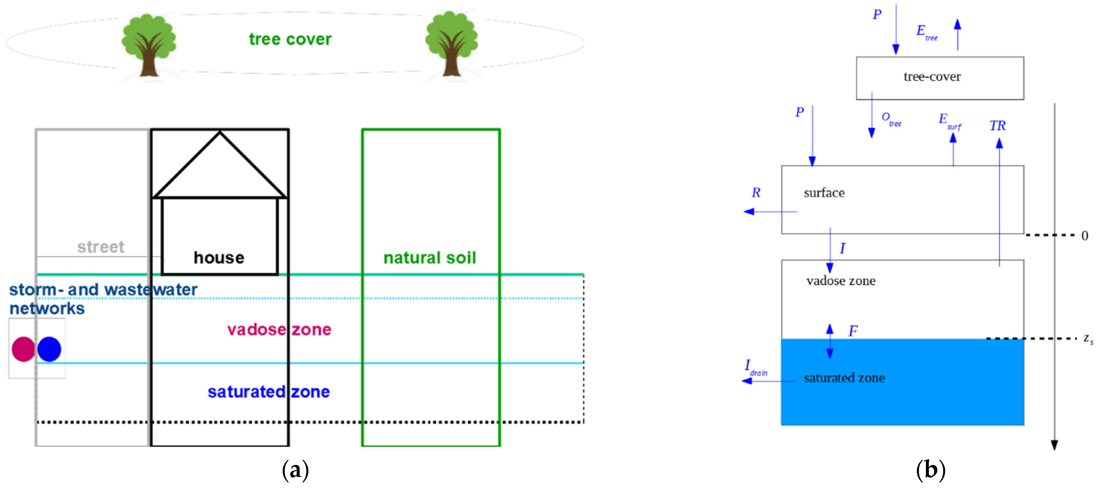
URBS-MO is a distributed hydrological model for urban catchments, and was initially developed by [24]. The unit element of this model is based on a cadastral parcel, combined with its adjacent street surfaces to form Urban Hydrological Elements (UHE), at which runoff is produced. An UHE is characterized by a set of geometrical attributes, including: the area, impervious surfaces (roofs and streets), tree-covered surfaces, length and slope, the connection point to the hydrographic network that is composed of the street surfaces and the sewer network, and the depth of the sewer segment. The cross-section of an UHE is composed of three vertical profiles representing roofs, streets and natural soil, respectively (Figure 1a), with each profile encompassing four superimposed and interacting reservoirs. The water flows and storages are computed on a 1D vertical scheme at each profile, including precipitation P, tree interception (P-O_tree), surface runoff R, infiltration I, evapotranspiration (E_tree, E_surf, TR), percolation F, and the groundwater drainage by the sewer network I_drain (Figure 1b). Modelling details on all of the processes parametrizations may be found in [24].

The two-reservoir structure of the subsurface created by the vadose zone and saturated zone makes it possible to describe two main variables of soil water: (i) the water content of the vadose zone, and (ii) the saturation level z_s. Specifically, the vadose zone receives infiltration I and provides water for tree transpiration TR. The saturation level is controlled by a saturated zone–vadose zone exchange flow F (percolation and suction). The possible drainage of groundwater by the sewer network (I_drain) is also modeled by an ideal-drain approach. Water exchanges within each UHE between the profiles are assumed to occur only in the saturated zone, and the average saturation level of each UHE is averaged at each time step. A key parameter of this water exchange in both the vadose and the saturated zone is the hydraulic conductivity. The hydraulic conductivity at saturation K_sat is represented by an exponentially decreasing curve, as inspired by TopModel [33]. Urban soils tend to be more compact with depth [34], and this assumption is suitable for these soil types:

K_sat(z) = K_se^−z/M,

(1)

where K_sat(z) (m/s) is the saturated hydraulic conductivity at depth z (m) below the ground’s surface, K_s (m/s) is the saturated hydraulic conductivity at the ground’s surface, and M (-) is a scaling parameter of the exponentiation.

In the end, the flow routing from each UHE to the catchment outlet is modeled by a Runoff Branching Structure (RBS), a vector map composed of streets and sewer segments [35]. The flow routing contains two modelling stages: (i) the routing of surface runoff from UHEs to sewer inlets along streets, as represented by travel time routing, and (ii) hydraulic routing inside sewers, modeled by the Muskingum–Cunge scheme, which is an approximate solution to the diffusive wave equation. In this manner, the discharge in any segment of the stormwater routing network at any time step can be calculated. URBS-MO can run continuously at small time steps (~minute) over a long time series (~several years). The model has been evaluated on two urban catchments of various land uses [24], and has shown its capability to describe thoroughly the hydrological behavior of an urban catchment.

Lateral groundwater flow is not modeled explicitly in URBS-MO, which may lead to an abrupt water table difference among the UHEs. A coupling between URBS-MO and MODFLOW was first implemented in [19,36], but this approach has not been successful due to the different soil parameterizations in both models.

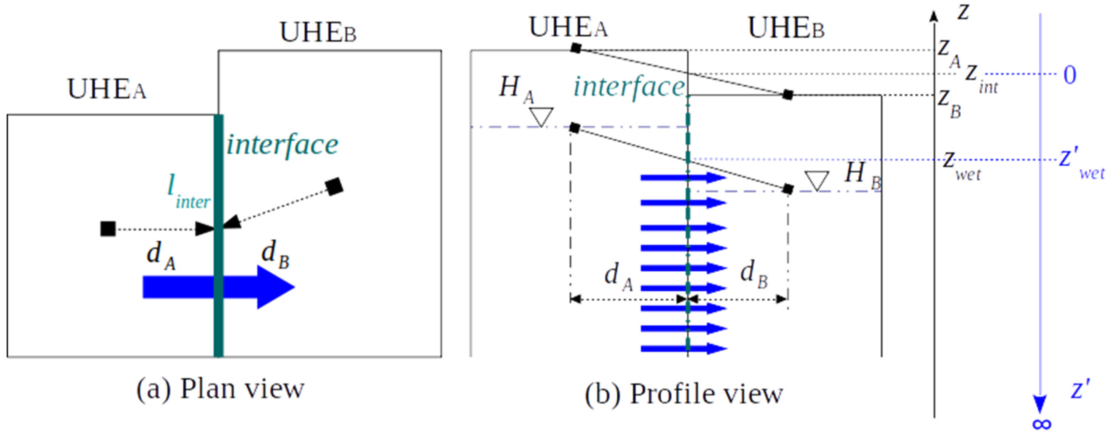
2.1.2. WTI

WTI, for Water Table Interface, is a module developed within the LIQUID hydrological modelling platform [37]. It computes the lateral flow between adjacent model units using Darcy’s law, with “model units” referring to agricultural fields, hedgerows and urban parcels. The module has proven to be able to compute adequately the flow exchanges between the model units [38].

The concept of the WTI module is illustrated in Figure 2. An interface “inter” is set between two adjacent model units A and B, which serves as the geometrical support for the computation of the groundwater flow $Q_{A\to B}$ (m³/s) between the model units by Darcy’s law:

$$Q_{A\to B}^{inter}=K_{inter}{A}_{inter}\overrightarrow{\nabla }H$$

(2)

where K_inter (m/s) is the hydraulic conductivity applied on the interface, A_inter (m²) is the wet section of the interface, and $\overrightarrow{\nabla }H$(-) is the hydraulic gradient between A and B, calculated as:

$$\overrightarrow{\nabla }H=\frac{H_A-H_B}{d_{AB}}$$

(3)

where H_A (m) and H_B (m) are the groundwater levels in A and B respectively, and $d_{AB}$ (m) is the distance between the geometrical centers of the model units. The wet section is calculated as l_inter × (H_inter − H_bottom), where l_inter (m) is the length of the interface; H_inter (m) is the groundwater level at the interface, calculated by a linear interpolation between H_A and H_B; and H_bottom (m) is the elevation of the bedrock.

2.2. Integration of the WTI into URBS-MO

2.2.1. Mathematical Formulation of the Module Integration

The principle of integrating the WTI in URBS-MO is inspired by PUMMA (PeriUrban Model for landscape MAnagement) [38]. We introduced an interface between every pair of UHEs (Figure 2), across which lateral groundwater flows and the flux is calculated by Darcy’s law (Equations (2) and (3)). In terms of geometry, the interface is a line seen from above (Figure 2a), and a surface seen in the soil column (in the plan (x,y), not shown in Figure 2). Groundwater levels H_A and H_B were assumed to be uniform in each UHE. The distance between the centers of the UHEs dAB is approximated by dA + dB, with dA and dB being the distance between the geometrical center of the interface and that of the UHEs.

A tricky problem concerns the hydraulic conductivity K_inter and the wet section A_inter, due to the fact that the soil is not limited at the bottom in URBS-MO. As a matter of fact, the saturation level was expressed by a “saturation deficit”, a concept defined as the water depth needed to saturate the vadose zone, in reference to the ground surface. Consequently, the interface is not limited at the bottom, either. From a model compatibility point of view, it makes sense to retain the exponential decrease of the hydraulic conductivity in WTI. It is thus delicate to estimate a mean value for K_inter assigned on the interface. This problem was dealt with in the PUMMA model by assuming the existence of bedrock at the depth of the sewer segment [38]. In the present study, we proposed a new solution, which consists of writing the flow equation in the form of integration. The element volume for the integration is the flow volume through an elemental surface area of the interface. The upper border of the integration is the water table at interface H_inter, and the lower border is infinity.

As illustrated in Figure 2, the WTI flow was computed, as were all other processes, in the initial z’-downward system. The referential level of each interface was set at its ground surface, and was obtained by the distance-weighted elevation of UHE_A and UHE_B. The water table at the interface z’_wet (m) was calculated by the distance-weighted groundwater level of the two UHEs, but it was expressed in the z’-downward system. The NGF system (the French general standardizing altitude system) was chosen as the z-upward coordinate system for the results analysis.

Equation (2) can be written as an integral, in the z-downward system, from z′_wet to the infinity, as:

$$\begin{gathered} Q_{A\to B}^{inter}=\underset{z{\prime }_{wet}}{\overset{\infty }{{\displaystyle \int }}}{K}_s^{nat}{e}^{-z\prime /M}·\frac{H_a-H_B}{d_A+d_B}·d{A}_{inter} \\ \hspace{1em}\hspace{1em}\hspace{1em}\hspace{1em}\hspace{1em}\hspace{1em}\hspace{1em}\hspace{1em}=\underset{z{\prime }_{wet}}{\overset{\infty }{{\displaystyle \int }}}{K}_s^{nat}{l}_{inter}{e}^{-z\prime /M}·\frac{H_a-H_B}{d_A+d_B}·dz\prime \end{gathered}$$

(4)

where K_s^nat (m/s) is the saturated hydraulic conductivity at ground level, and M (-) is the scaling parameter of K_s^nat.

The anti-derivative writing of Equation (4), along with the approximation that the hydraulic gradient between the two UHEs is constant in depth, lead to:

$$\begin{gathered} Q_{A\to B}^{inter}=K_s^{nat}{l}_{inter}\frac{H_a-H_B}{d_A+d_B}\underset{z{\prime }_{wet}}{\overset{\infty }{{\displaystyle \int }}}{e}^{-z\prime /M}·dz\prime \\ \hspace{1em}\hspace{1em}\hspace{1em}\hspace{1em}\hspace{1em}\hspace{1em}\hspace{1em}\hspace{1em}=-K_s^{nat}{l}_{inter}\frac{H_a-H_B}{d_A+d_B}{\left[e^{-z\prime /M}\right]}_{z{\prime }_{wet}}^{\infty } \end{gathered}$$

(5)

Because $e^{-z\prime /M}$ tends towards 0 when z′ tends to infinity, the anti-derivative is ultimately given by:

$$Q_{A\to B}^{inter}=K_s^{nat}{l}_{inter}\frac{H_a-H_B}{d_A+d_B}{e}^{-z{\prime }_{wet}/M}$$

(6)

Equation (6) is the final equation by which the water flow between two adjacent UHEs is computed at their interface.

Finally, in order to have the possibility to take into account an eventual anisotropy of the soil in URBS-WTI, a new parameter, K_s^lat, was introduced in order to represent lateral (horizontal) saturated hydraulic conductivity. Thus, if this option is enabled, K_s^lat is substituted for K_s^nat in the previous equation.

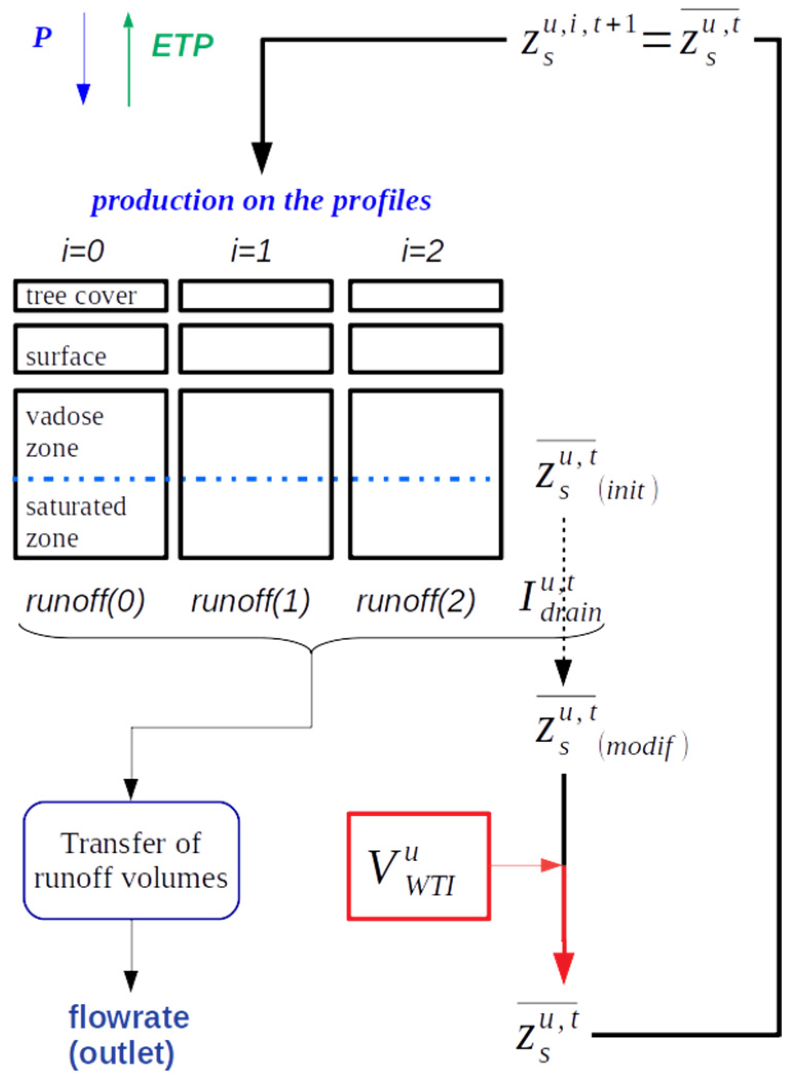
2.2.2. Spatial and Temporal Discretization of the Module Integration

The WTI module integration slightly modifies the spatial and temporal discretization and the routing scheme of URBS-MO (Figure 3). In URBS-MO, at each time step t and for a given UHE u, the runoff production is simulated at each of its vertical profiles i. The saturation level of each profile $z_s^{u,i,t}$ is then updated by transpiration TR and the flow F between the vadose zone and the saturated zone. The saturation level at the UHE scale $\overline{z_s^{u,t}}$_(init) is then given by the area-weighted mean of the saturation levels of the three vertical profiles. This averaged saturation level is later modified by the sewer drainage $I_{drain}^{u,t}$ into $\overline{z_s^{u,t}}$_(modif). At the beginning of the next time step, the saturation level of each profile z^u,i,t+1 is renewed to $\overline{z_s^{u,t}}$.

The integration of WTI followed the $I_{drain}^{u,t}$ computation. Explicitly, within each time step, once the saturation levels of all of the UHEs are updated by the drainage flow $I_{drain}^{u,t}$, the WTI module was applied to all of the interfaces iteratively. As illustrated in Figure 2b, on any interface inter of the adjacent UHEs of u, the computation of the transferred water volume from A to B—where A = A(u) is any adjacent UHE of u and B = u —was implemented through Equation (6). $Q_{A\left(u\right)\to u}^{inter}·\Delta t$ is preceded by the ‘+’ sign when the flow is from A(u) to u, and the ‘-‘ sign when the flow is from u to A(u). Once the iteration on the interfaces is complete, the transferred water volume $V_{WTI}^u$ of a given UHE u is obtained by the sum of $Q_{A\left(u\right)\to u}^{inter}\Delta t$:

$$V_{WTI}^u={\displaystyle \sum }_{inter=1}^{n_u}\left(Q_{A\left(u\right)\to u}^{inter}\Delta t\right)$$

(7)

where n_u is the number of the interfaces of u.

Finally, the saturation level of u was updated by $V_{WTI}^u$:

$$\overline{z_s^{u,t}}={\overline{z_s^{u,t}}}_{\left(modif\right)}+\frac{V_{WTI}^u}{S{A}^u·{\theta }_s}$$

(8)

where SA^u (m²) is the surface area of u, and θ_s is the moisture content at the saturation, parameter of the model. $\overline{z_s^{u,t}}$ is then assigned to each profile at the beginning of the next time step.

As such, the groundwater transfer module WTI was integrated in URBS-MO. The mathematical adaptation enables the modelling of the water flow in the saturated zone in a suitable method. Specifically:

• The temporal and spatial discretizations in URBS-MO based on UHE are untouched.
• The conception and parameterization of soil in URBS-MO are kept, which assures the model compatibility and avoids introducing supplementary model parameters.
• It uses a simple modelling approach based on Darcy’s law and the law of mass conservation, which are governing equations of a hydrological system [39].
• The general model structure is not modified.

The integration was initially tested on a sample of 5 UHEs, and the numerical computation results were verified.

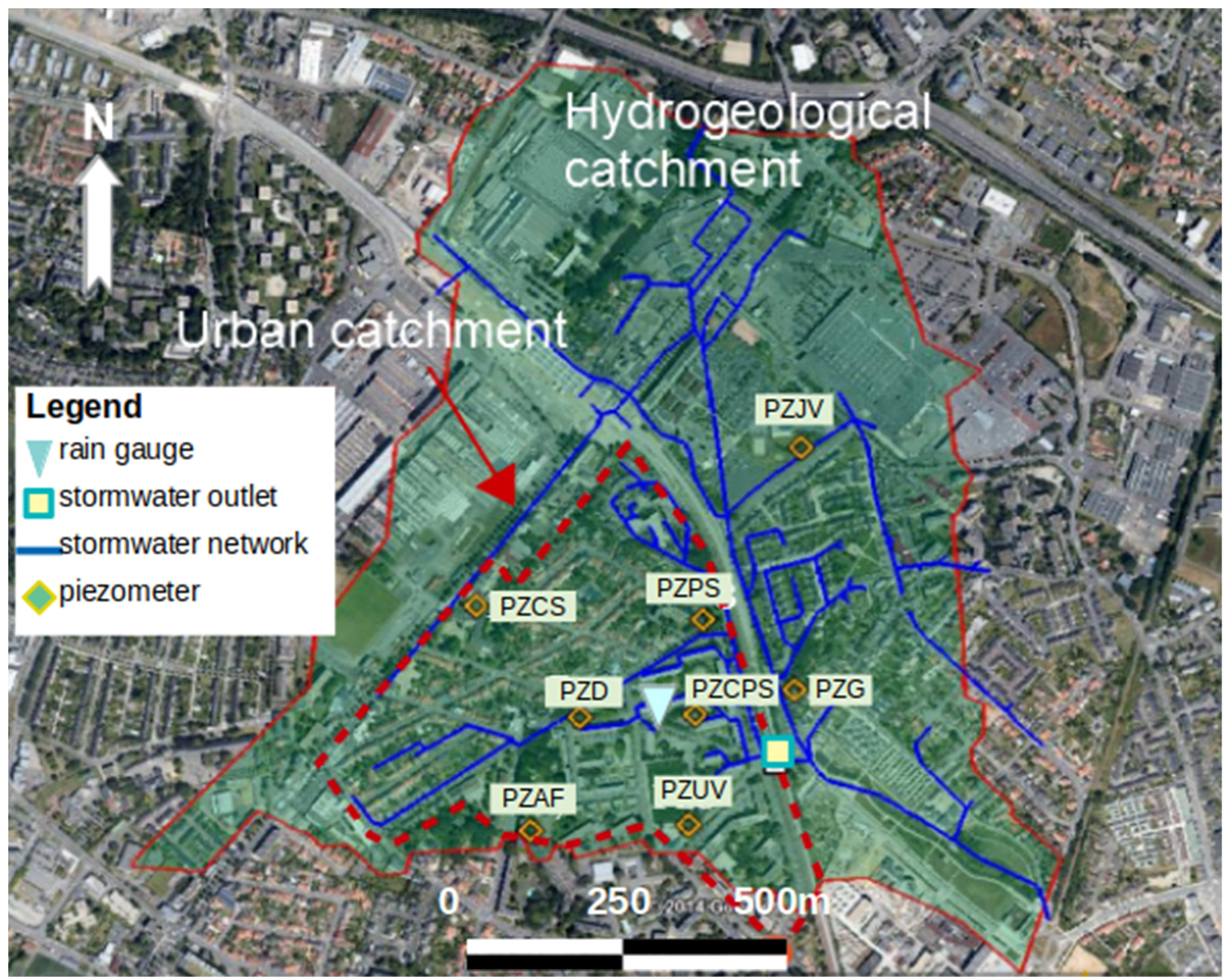
2.3. Case Study

The urban catchment of Pin Sec (31 ha, the dotted line in Figure 4) is located in the east of Nantes city in France, between the rivers Loire and Erdre. It comprises a separated sewer network for stormwater and wastewater. The land cover is shared by small collective and individual dwelling areas. The impervious ratio is approximately 45%, and the mean slope is 1.1% from north-west to south-east [40,41]. The outlets of the storm- and wastewater networks are located to the south-east of the catchment, at a distance of 300 m (Figure 4). The total length of the stormwater network is 4 km, and that of the wastewater network is 7.3 km. The outlet of the stormwater network is an underground pipe that drains into the Gohards stream. The urban catchment is contained within a ridgeline-defined hydrogeological catchment of approximately 133 ha (Figure 4).

Pin Sec is underlaid by the Massif Armoricain formation. Three geological layers can be distinguished: silt, alluvium and mica schist. An unconfined aquifer lies in the deeper ground. According to [42,43], water is mainly stored in altered rocks, moving through rock cracks and fissures. These authors studied the aquifer within the city of Nantes, and observed that the groundwater table fluctuated between −2.5 m and −5.7 m during the winter. Within Pin Sec, the groundwater table is lower, varying between −3 m and −4 m. Mougin and Conil [43] indicated that the aquifer is naturally drained by the rivers Loire and Erdre.

Pin Sec is an observation catchment of ONEVU (Observatoire Nantais des EnVironnements Urbains), an in-situ environmental observatory in hydrology, micro-meteorology, climatology, and air, water and soil quality. The hydrological measurements (from 2006 onwards) include the rainfall, flow rates at the storm- and wastewater outlets, and groundwater monitoring by a network of piezometers. The daily potential evapotranspiration (PET) rate is provided by Meteo France [44], and is interpolated at an hourly time step with the assumption of a sinusoidal profile during daytime. The piezometers are installed in the altered mica-schists. No impermeable layer exists between the ground surface and the measured depth, and the measured level is the shallow free-water table, which varied between −4.5 m and −0.5 m during 2006–2010.

The hydrogeological catchment of Pin Sec comprises 875 parcels, corresponding to UHEs for the URBS model, varying in size from 1.5 m² to 117,724 m² (Figure 4). The total area of 133 ha encompasses 15% streets, 19% building roofs, 12% within-parcel pavements (pathways, parks), and 54% natural permeable surfaces, encompassing private and public green areas and individual gardens. In total, 1/3 of the natural surface is covered by trees, and this fraction is much lower on impervious surfaces, at only 1.6%. The geographical data of the parcels needed for the execution of URBS-WTI is provided by GIS (Geographical Information Systems) urban databanks.

2.4. Model Setup

The integrated model URBS-WTI was run continuously on the 5-year period from 1 January 2006 to 31 December 2010, in 5-min time steps. Continuous rainfall and PET were uniformly applied on the catchment. Defining boundary conditions for the subsurface flow at the limit of the Pin Sec hydrological catchment is difficult due to the unavailability of detailed soil characteristics and hydrogeological data. In order to overcome this difficulty, the model was applied at the entire hydrogeological catchment, to which a zero-flow boundary condition was applied for groundwater flow. Based on the measurement data, Le Delliou [36] made an estimation of the water balance for the Pin Sec catchment, and stated that the average groundwater flow out of the catchment was about 0.023 mm/day.

Two urban catchments in the neighborhood of Pin Sec, Rezé and les Gohards have been subjected to previous applications of URBS-MO [24]. Physical model parameters have been calibrated on these catchments. Given that the geological conditions of Pin Sec are the same as those catchments, we began our simulation by taking the parameter values calibrated by [24]. Given the large number of the physical parameters, an exhaustive list of parameters is omitted here, and can be found in [24]. Among the 15 model parameters,

Table 2. Parameters used within the catchment modelling: the value for the initial run and the range for the sensitivity analysis.

Parameter	Unit	Initial Value	Range
Ksnat & Kslat, Hydraulic conductivity at saturation at ground surface	m/s	1.3 × 10−5	[1 × 10−6, 1 × 10−4]
M, Scaling parameter for the hydraulic conductivity curve	-	0.2	[0.1, 10]
$\lambda$, Coefficient of groundwater drainage by sewer network	-	17	[0, 150]
z0, Initial saturation level	m	−1.7	[−0.05, −2]

only focuses on the parameters that operate on the WTI module. These parameters will be subjected to a sensitivity analysis later.

The saturation depth was uniformly initialized (z⁰) over the catchment. Information on the groundwater level at the beginning of the simulation period (1 January 2006) is unavailable. The mean level measured by the piezometers on 1 January 2007, −1.7 m, was thus used for z⁰.

The modelling outputs at every time step are comprised of:

–

flows (infiltration, evapotranspiration, etc.) and the storage of the reservoirs at the catchment scale

–

the runoff volume at the outlet of the stormwater sewer network of the urban catchment

–

the groundwater level at every UHE.

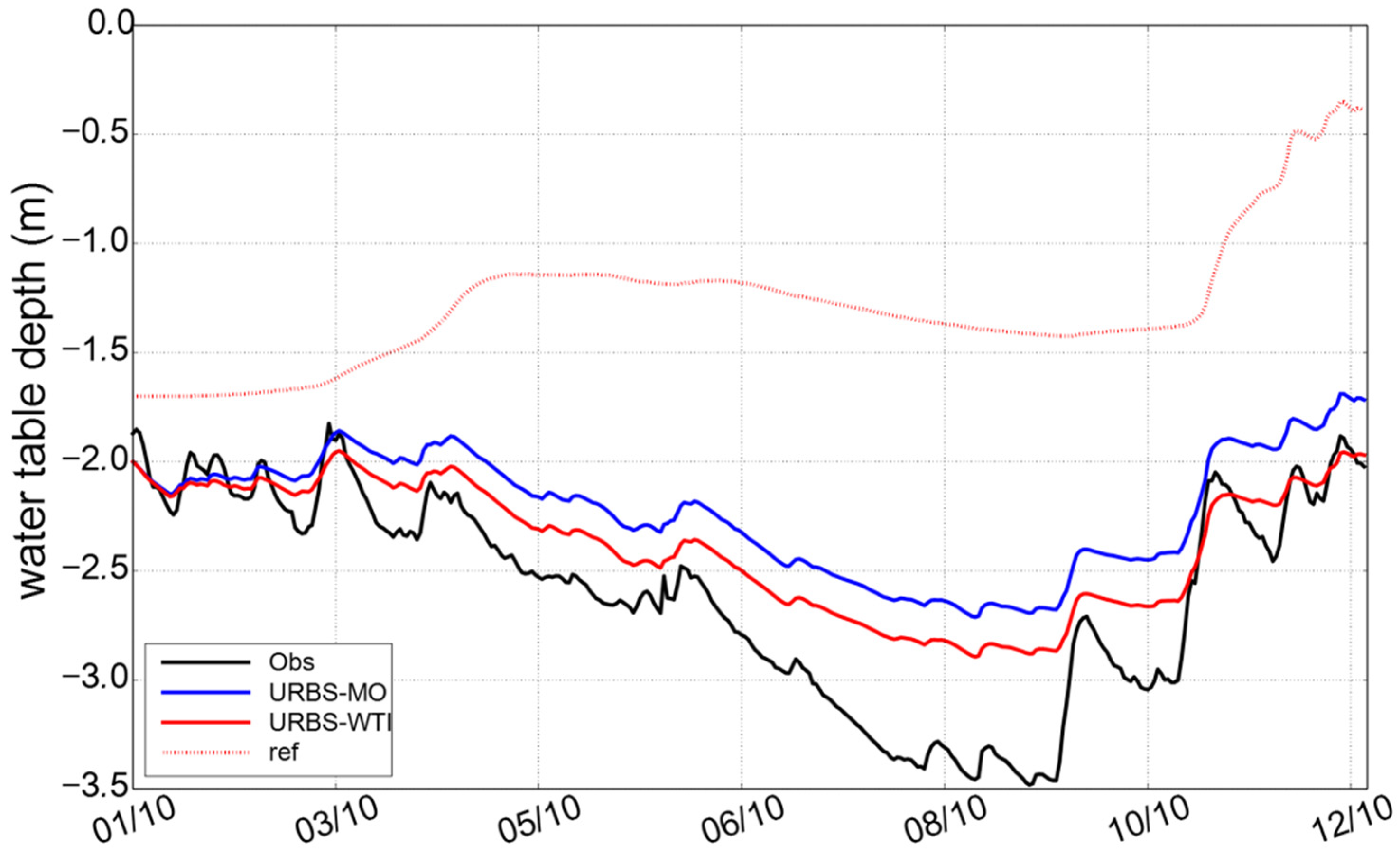
2.5. URBS-WTI Model Evaluation Methodology

For the evaluation of the model performance, these modelling outputs were analyzed thoroughly. The first type of output was examined through a water balance analysis, encompassing the following variables: Q^hou, Q^str, and Q^nat, the runoff from the three land-use types (house roof, street, natural soil); Q^drain, the groundwater drainage by the sewer network; E, surface evaporation; TR, transpiration; ∆s, the storage variation in the soil between the end and the beginning of the simulation period; and P, rainfall.

Because runoff is the most widely used output to evaluate hydrological models, groundwater level is rarely used in model calibration and validation. Here, we based our evaluation on a groundwater level comparison. 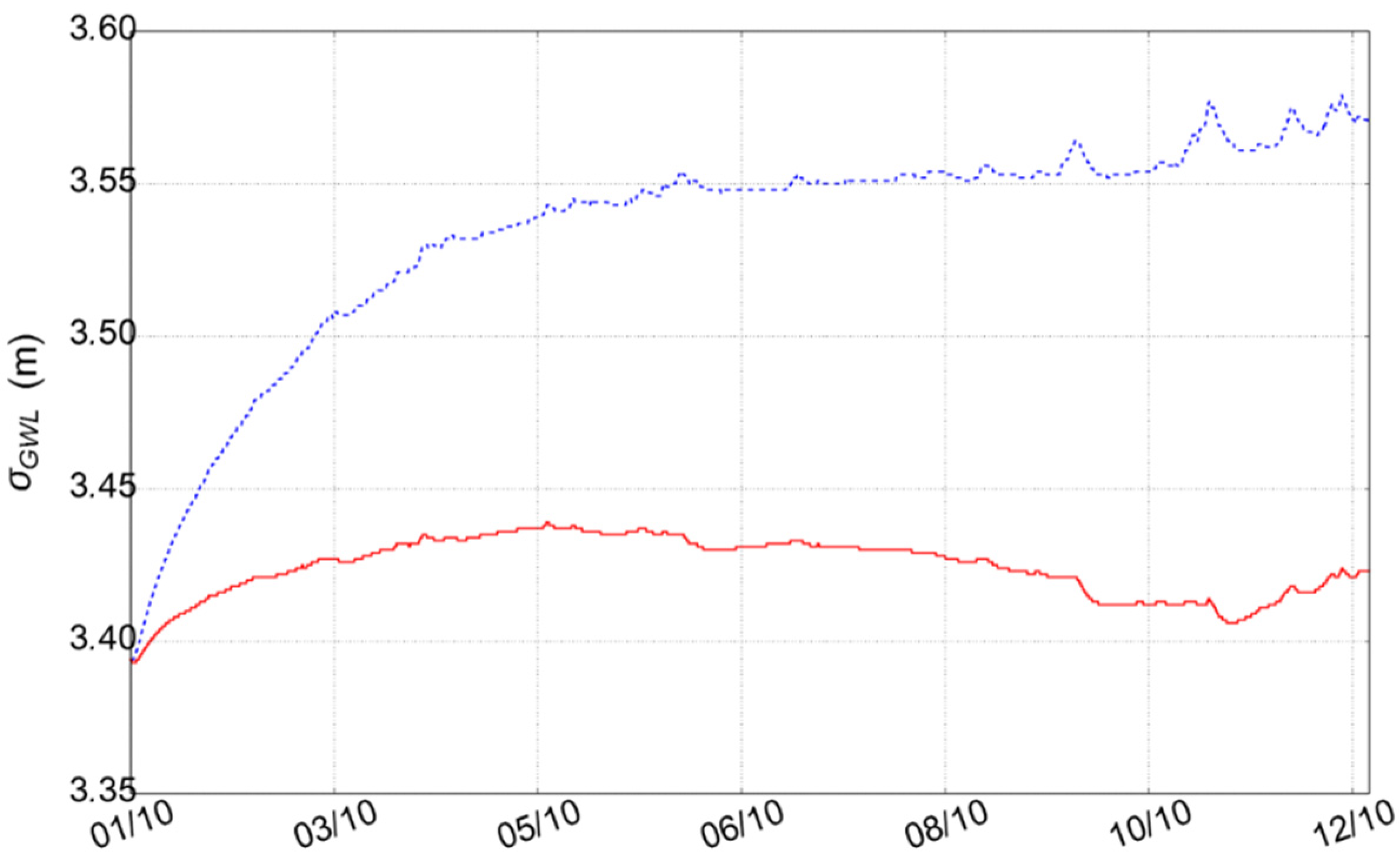In addition to the visual inspection of simulated and observed groundwater level curves, three traditional comparison criteria were used to estimate the error between the simulated and observed levels: the bias error C_b, the Nash–Sutcliffe efficiency C_nash [45], and the coefficient of determination R² (see Appendix A for details). Comparison between the modelling results of URBS-MO and URBS-WTI can indicate the impacts of the WTI module on the model behavior. In order to evaluate these impacts on groundwater levels at the catchment scale, an adapted criterion was added. The temporal variation of the standard deviation σ of the simulated groundwater levels of the UHEs is calculated for each time step t as:

$${\sigma }_{GWL}^t=\sqrt{\frac{{{\displaystyle \sum }}_{u=1}^{n_{UHE}}{\left(z_s^{u,t}-\overline{{z_s}^t}\right)}^2}{n_{UHE}}}$$

(9)

where ${\sigma }_{GWL}^t$ is the standard deviation of the groundwater levels, z_s^u,t (m) is the groundwater level of UHE u in the NGF system, $\overline{{z_s}^t}$ is the mean groundwater level of all of the UHEs at time t, and n_UHE is the number of UHEs. The more ${\sigma }_{GWL}^t$ is low, the more the groundwater table is homogeneous throughout the catchment.

Additionally, the simulated and observed flowrates in the stormwater network at the catchment outlet were compared by using the three criteria C_b, C_nash and R², which were calculated both during continuously during the whole period and during storm events only.

All of these criteria were applied at a 5-min time step for runoff series at the outlet of the rainwater network, and a 20-min time-step for groundwater levels.

The evaluation is composed of three steps of work: (i) a sensitivity study from an initial parameter set, (ii) a manual parameter calibration and a detailed analysis of the calibrated run results, and (iii) a validation step on a different modelling period.

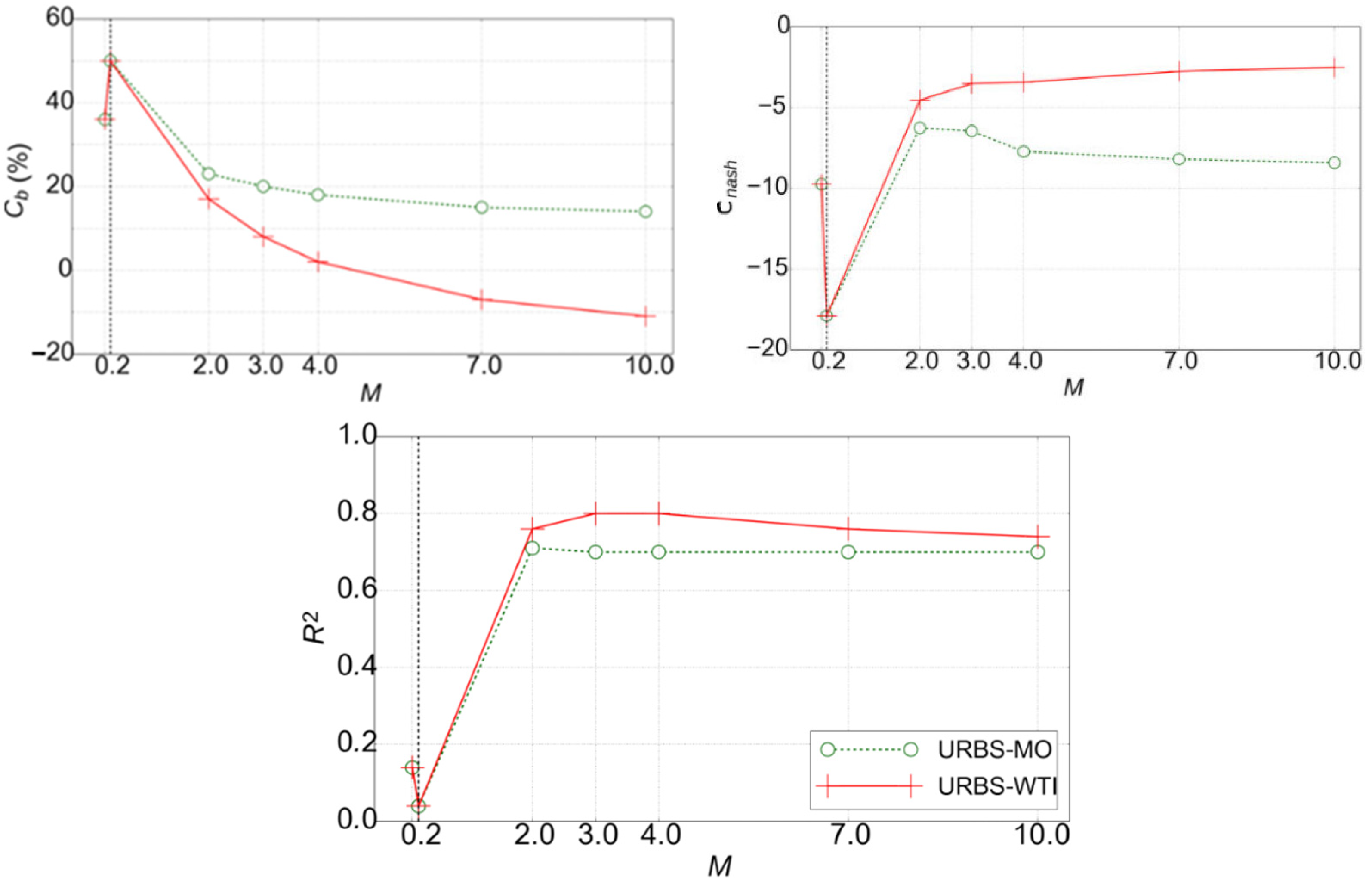
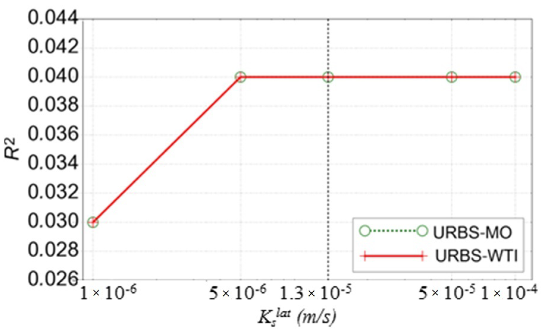
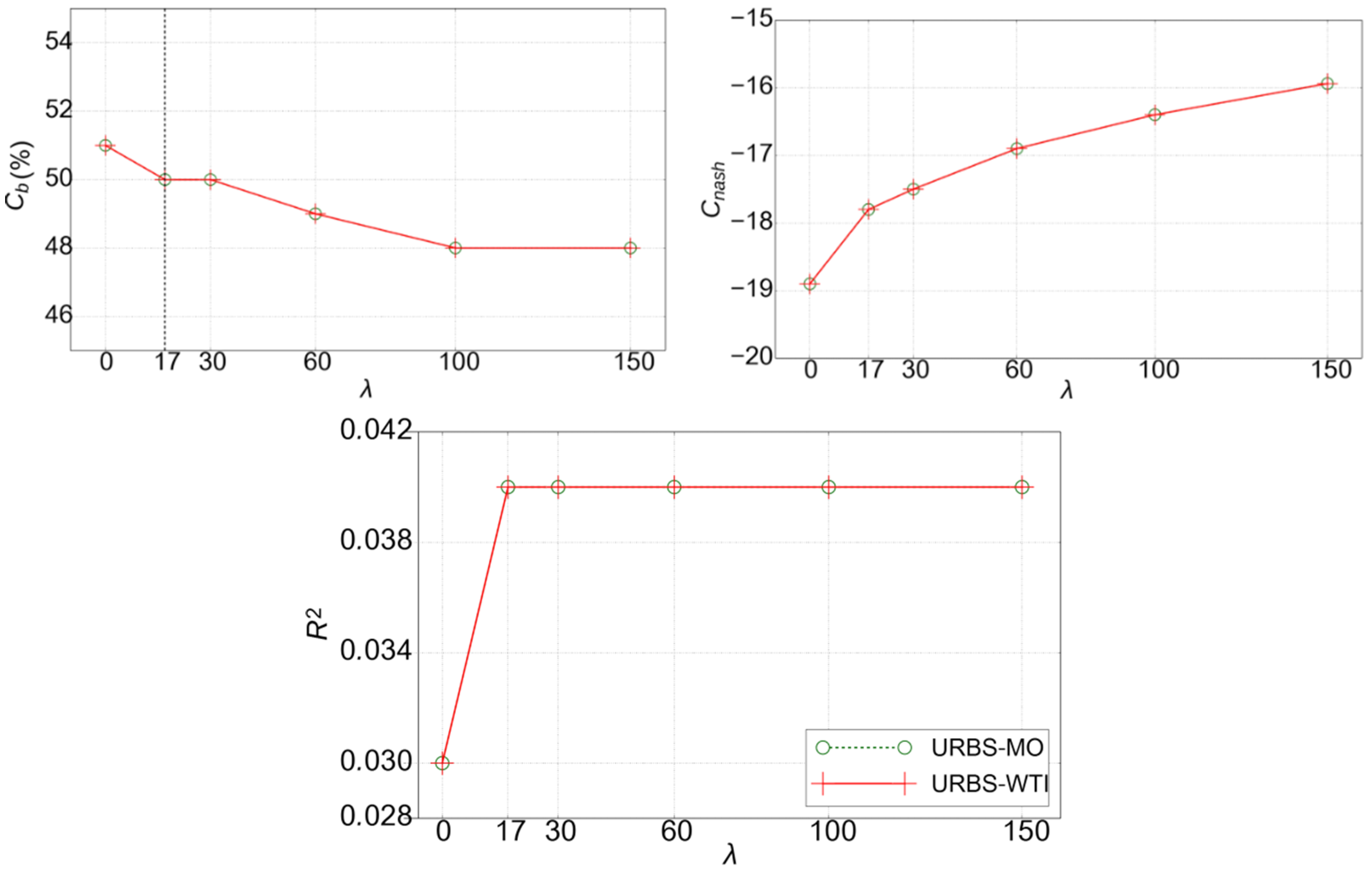
(i) The sensitivity analysis of the model parameters was carried out in order to explore the following questions. To what extent is the model URBS-WTI sensitive to the parameters controlling the groundwater compartment modelling? Is this sensitivity different from that of URBS-MO alone? What are the most influential parameters for this catchment, especially related to the integration of the WTI module in the URBS Model? Three parameters with an eventual impact on the WTI module were analyzed: (i) the lateral saturated hydraulic conductivity at natural ground surface K_s^lat, (ii) scaling parameter M of the exponential decrease of K_s^nat, and (iii) the coefficient of groundwater drainage by sewer networks λ. K_s^lat and M operate directly on the WTI flow; λ regulates the groundwater drainage flow, and thus influences the groundwater level and subsequently the lateral groundwater flow. The sensitivity of the initial homogeneous saturation condition of the catchment z⁰ was tested too, because it appeared as an essential parameter governing the groundwater level modelling in the previous application of URBS-MO [24]. The one-factor-at-a-time method [46] was used for the sensitivity analysis, carrying out simulations by varying one parameter at a time. The three criteria C_b, R² and C_nash were calculated between the mean simulated and observed groundwater levels. Due to the time and memory consumption of the simulations, the sensitivity analysis was carried out on a one-year simulation (2010).

(ii) The sensitivity analysis performed will with the manual calibration step, as the optimized parameter values are deduced from the best criterion values obtained for each parameter. The main objective of this calibration step was not to obtain absolutely the best parameter set but to understand the impact of each parameter on the model outputs in order to deduce a good performance of the model, keeping in mind its physical principles [38]. For this reason, no automatic calibration was chosen. The calibration period was the same as that chosen for the sensitivity analysis, i.e., the year 2010.

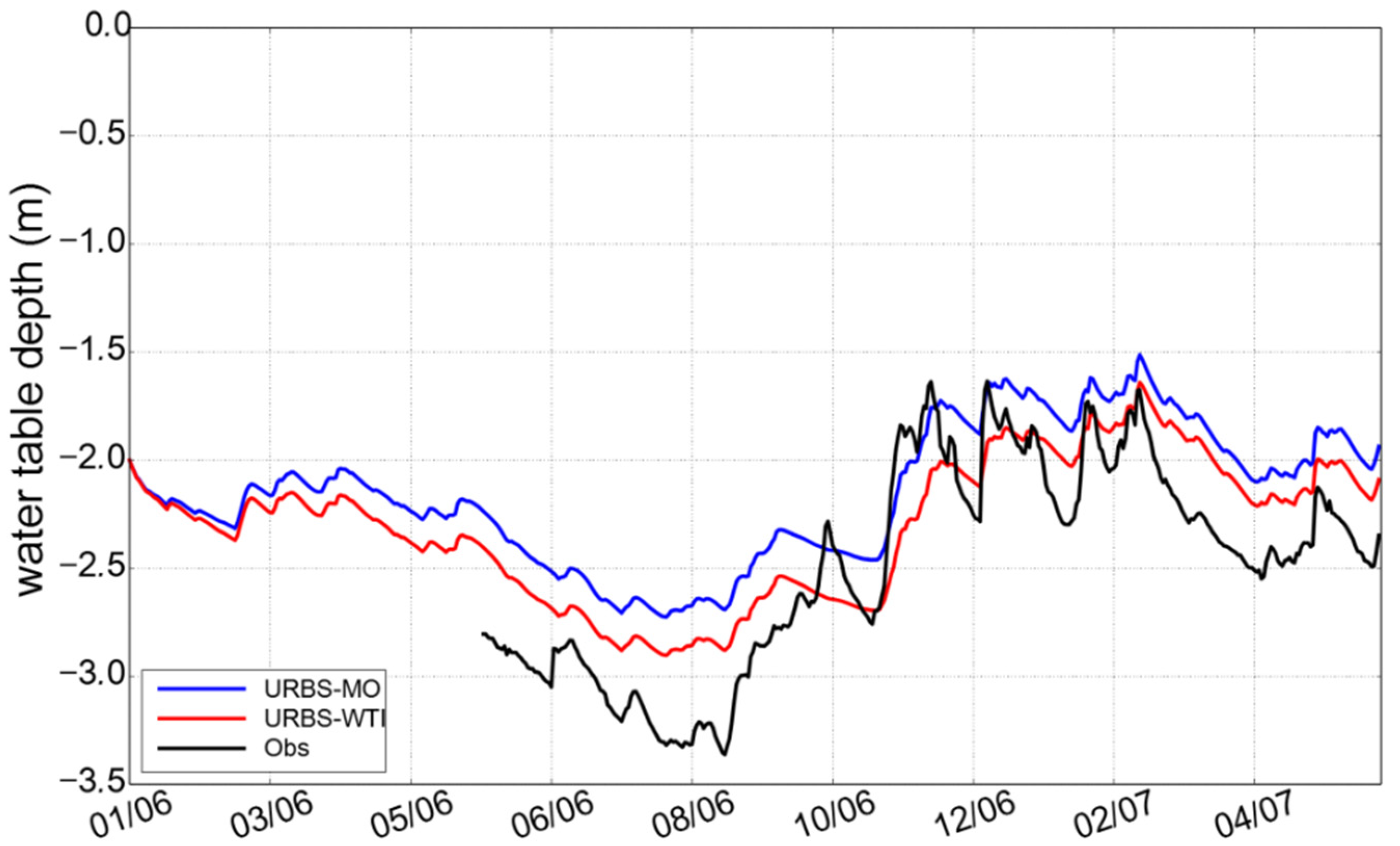
(iii) In the end, the model was evaluated through a validation period of one year and a half (1 January 2006–18 June 2007); this period of time was chosen because of the high quality of the groundwater level data from 15 May 2006 to June 2007, with the first 6 months of 2006 being used as a warming period.

3. Results

3.1. Sensitivity Analysis

The simulated groundwater level was sensitive to the initial saturation depth z⁰ (Figure 5). For z⁰ higher than −1 m, the model needs a “warm-up” period of about 3 months. Beyond 3 months, the model assesses the same groundwater level. For z⁰ lower than −1.5 m, the effect of z⁰ was observed not only at the beginning but for the entire year simulation period. Especially when z⁰ is below −2 m, the model needs almost one year to “warm-up”.

The simulated groundwater level did not show a high sensitivity to the lateral saturated hydraulic conductivity K_s^lat (Figure 6). The variations of the criteria were small, and the groundwater levels were, overall, overestimated (50%). The same statements can be found for λ (Figure 7), i.e., weak sensitivity, the overestimation of the groundwater levels, no effect of the WTI module, and slightly better results from a higher λ.

The results for M were different (Figure 8). C_b varied in the range 50–15% for URBS-MO, and 50–10% for URBS-WTI. C_nash was still weak (negative), but tended towards better values with a higher M, especially for URBS-WTI. R² reached relatively high values (around 0.8) with a higher M, both for URBS-MO and URBS-WTI. Furthermore, an increase in the value of M allowed URBS-WTI to produce higher efficiency values than URBS-MO. M is the scaling parameter of the exponential decrease of the saturated hydraulic conductivity (Equation (1)). The higher the value of M, the less rapidly the hydraulic conductivity decreases with the soil depth. The results for M signify that the groundwater level simulation may be better when the simulated flows in the soil, including the lateral WTI flow in the saturated zone, are increased. Additionally, this step highlighted the influence of the WTI module.

Despite the fact that the model sensitivity was not strongly modified by WTI, WTI tended to improve the groundwater level simulation with parameter values enforcing the soil flows. Notice that the results may be influenced by the initial parameter set chosen for the sensitivity analysis.

3.2. Calibration Stage

A series of supplementary tests was carried out by taking high values of M and λ, seeking to enforce the soil flows. In parallel, z⁰ was adjusted with the changes in M and λ. A higher z⁰ allowed the model to reproduce the observed dynamics of the groundwater level, but lead to its overestimation. Even with high values of M and λ, the over-estimation could not be corrected if z⁰ was set too high (less deep than 1 m). On the other hand, a lower z⁰ allowed for a better fit between the simulated and observed groundwater level but erased the observed oscillations if the modeled soil flows were not strong enough. It is supposed that this problem can be solved with longer simulation periods.

Ultimately, M was set to 2 and λ to 30, with z⁰ = −2.0 m; this set of parameter values assessed satisfactory simulation results, which are detailed in the following section.

3.2.1. Groundwater Levels

The mean groundwater level of the piezometers, simulated by a calibrated run of URBS-MO and URBS-WTI, was compared to the measured one (Figure 9). Compared to the first run, the simulation quality for the groundwater level was improved. If the simulated levels still do not fit perfectly the observed one, the initial over-estimation is largely corrected. C_b was reduced from 51% to 14% and 8%, respectively, for URBS-MO and URBS-WTI (

Table 3. Comparison criteria for the simulated mean groundwater levels from the calibrated run of URBS-MO and URBS-WTI, compared with the initial run results. The calibration period was 2010.

Parameter Set	Cb	Cnash	R2
Initial run URBS-MO	51%	−8	0.01
Calibrated URBS-MO	14%	0.15	0.91
Calibrated URBS-WTI	8%	0.62	0.96

). Initially negative, C_nash grew to positive values, with that of URBS-WTI reaching 0.62. Both URBS-MO and URBS-WTI showed higher R². However, the dynamics of the measured water table variation were not completely reproduced by the model, especially during low summer levels, and this could be due to the overly simple way of representing evapotranspiration in the model.

URBS-WTI showed a better performance than URBS-MO. The WTI module allowed, to a certain extent, the correction of the over-estimated groundwater levels. Correspondingly, the criteria C_nash and R² were much improved. These results were, overall, in the same order of magnitude that previous modeling results obtained with the dynamic coupling of surface hydrological models with groundwater models, such as SWMM-MODFLOW [29] and WEAP-MODFLOW [27].

The standard deviation of the simulated groundwater level ${\sigma }_{GWL}$ (Figure 10) showed that URBS-MO rises continuously, especially during the first part of the year, with little peaks in response to rainfall events, especially at the end of the year. These peaks represent the stronger variability of the groundwater level between each UHE, which is explained by the contrasting soil flows through the UHEs during a rain event (infiltration, drainage by the network, etc.). Simultaneously, ${\sigma }_{GWL}$ with URBS-WTI tends to be stable; this result confirms the capacity of WTI to homogenize the groundwater level between each UHE.

3.2.2. Water Balance

The water balance and flow rates assessed by the calibrated run of URBS-MO and URBS-WTI (

Table 4. Simulated water balance of the Pin Sec catchment given by a calibrated run of URBS-MO and URBS-WTI; all of the flow and storage components are expressed as a percentage of the total rainfall; the results given by the initial run are added. The calibration period was 2010.

Parameter Set	Qhou	Qstr	Qnat	Qdrain	E	TR	∆S
Initial run URBS-MO	16.7	10.6	1.2	4.2	5.9	38.1	22.9
Calibrated URBS-MO	16.7	10.3	0.1	27.9	5.7	31.9	6.8
Calibrated URBS-WTI	16.7	10.3	0.4	30.9	5.9	31.3	4.1

) showed that the runoff of natural surfaces Q^nat was almost zero. The groundwater drainage by sewer network Q^drain was quite large, at 27.9% and 30.9% of the total rainfall (given by URBS-MO and URBS-WTI, respectively). These values are consistent with the values estimated by [36]; this high drainage flow results in less storage variation (∆S). As the groundwater level is lower in the calibrated run, the transpiration (TR) and runoff on natural surface Q^nat were also reduced in comparison with the initial run.

The impact of WTI on the catchment water balance was not really significant. Runoff and evapotranspiration were not modified, due to the weak (even null) contribution of groundwater to these components; however, Q^drain slightly increased and storage ΔS decreased because the groundwater level is a key factor of these components.

3.2.3. Runoff at the Stormwater Network

The model’s calibrated run showed an under-estimation of the runoff volumes, both during storm events and for the whole period of time (

Table 5. Comparison criteria for the (a) ‘continuous’ and (b) ‘during storm events’ runoff volume at the stormwater network outlet of Pin Sec by the calibrated run of URBS-MO and URBS-WTI. The calibration period was 2010); the results given by the initial run are added.

Parameter Set	Cb	Cnash	R2
Initial Run URBS-MO	(a) −49%/(b) −20%	(a) 0.57/(b) 0.72	(a) 0.59/(b) 0.85
Calibrated URBS-MO	(a) −31%/(b) −6%	(a) 0.56/(b) 0.90	(a) 0.55/(b) 0.91
Calibrated URBS-WTI	(a) −25%/(b) −3%	(a) 0.57/(b) 0.91	(a) 0.56/(b) 0.92

). The better criterion values during storm events, similarly to those obtained by [24] for a smaller urban catchment at the same 5-min time step, showed the limited performance of the model during dry periods. The WTI module tends to reduce the underestimation of runoff volumes thanks to an increase of the groundwater drainage by the network. Only the bias criterion C_b was consequently affected by both the WTI module introduction and the calibration stage.

3.3. Validation Stage on the Groundwater Levels

The validation stage was run for the 1 January 2006–18 June 2007 period (the measurements started only on 15 May 2006). The model, overall, retained its performance in groundwater level modelling (Figure 11). The observed seasonal variations were well reproduced by both the URBS-MO and URBS-WTI models, and the simulated peaks in winter matched the measured ones well. Bias error C_b was still weak, and was very similar to the one of the calibration period; C_nash was slightly better, and R² remained relatively high (

Table 6. Comparison criteria for the simulated mean groundwater levels given by the calibrated run of URBS-MO and URBS-WTI. The validation period was 2006–2007.

Model	Cb	Cnash	R2
URBS-MO	14%	0.30	0.87
URBS-WTI	7%	0.66	0.80

). URBS-WTI showed a better performance, with C_nash reaching 0.66, compared to 0.30 for URBS-MO. However, both models still failed in reproduce the low summer levels in the observation curve. These modelling results for a period other than the calibration period illustrated the robustness of the model.

4. Discussion

4.1. Model Sensitivity

The overall results of the sensitivity study show that the model sensitivity is not greatly impacted by the WTI module. The WTI module does not change the general behavior of the URBS model, except when considering the saturated hydraulic conductivity of soils. It is worth noting that we systematically examined the water balance assessed during the sensitivity study. This variable affords an insight into what happened in the model mechanism with a parameter change. We believe that this approach is crucial in order to understand the model and module behavior, especially when groundwater is dealt with.

4.2. Parameter Calibration

The parameter calibration was based on the groundwater level. This approach, although it is not common in urban hydrology, makes sense because we want to evaluate the groundwater flow module WTI. It was not always easy to observe obvious trends of the simulation quality with the parameter changes. For example, while strong values of M improve C_b and C_nash, they deteriorate R². There seems to be a balance between “magnitude” and “dynamics”. If a parameter change tends to bring closer the simulated curve to the observed one, it may not be able to reproduce the observed dynamics by giving a flat simulated curve.

On the other hand, because the analysis was conducted with the one-factor-at-a-time method, concluding that the best parameter set is the combination of the best value of each parameter can be unwise. If two parameter changes can both improve the simulation quality by impacting the flow in a similar way or an opposite way, their combination can lead to an over-correction or an offset.

Another difficulty lies in the heterogeneity of the piezometric observation, probably due to the complexity of the urban surface and subsoil. This current calibration stage was led by considering a spatially homogenous parameter set. Additional calibration results (not presented here) have proved that the optimal values of M and K_s^nat could change if we focused on a specific piezometer, and that the simulation improvements for certain piezometers were always at the detriment of the others. The possibility to support the integration of distributed parameters could be a valuable subject for future model development.

The set of parameters which was ultimately chosen is a result of this manual calibration stage. The general feeling we have is that the initial parameters, which were calibrated in the neighborhood catchment of Pin Sec, lead to very weak water flows. If we set a high initial saturation level, the groundwater level is over-estimated (as shown by the results of the model’s initial-run) due to an overly weak groundwater drainage flux; if we set a low initial saturation level, the mean groundwater level is no longer over-estimated, but its dynamics in measured variations disappear. Consequently, we had to adjust the parameters in such a way that the simulated flows were enforced, in combination with a suitable value for the initial saturation level.

4.3. WTI

The module’s WTI was integrated into the structure of URBS-MO via an adapted mathematical formulation. Compared to approaches favoring coupling URBS-MO with a groundwater model [36], this integration has the advantages of retaining the initial model conception and parameterization, and not causing temporal and spatial discretization conflicts. The calibrated parameters allow the module to better reproduce the observed groundwater level. The homogenization effect of the module was evaluated by the standard deviation of the levels of the UHEs, proving the relevance of this WTI module for a more realistic groundwater level simulation. This approach could be much enhanced by considering a spatial distribution of soil characteristic parameters within a catchment. Moreover, a more sophisticated analytical method might provide more convincing elements, for example with a better consideration of the vadose zone–saturated zone interactions, or by taking into account the possible stratification of the soil layers. However, appropriate data are missing for a better description of the urban soil features, which can be highly variable within small spatial scales [47].

5. Conclusions

This study allows us to integrate an existing groundwater module WTI into the physically-based distributed urban hydrological model URBS in order to improve its representativeness of the lateral saturated flow and groundwater level variation. An adapted mathematical formulation was realized for the WTI module, which allows us to maintain the conception and parameterization for the subsurface in the model URBS. Based on initial parameters derived from previous studies on the model, a sensitivity analysis was realized with the manual calibration of the parameters that have an impact on the groundwater module. This calibration stage used the groundwater level as the main metric, which is new in the field of hydrological modelling. The ensemble of model outcomes—including the water balance, flow rates and groundwater level—have been analyzed using one-factor-at-time method.

The results showed that the general URBS behavior and its sensitivity to the tested parameters were not significantly changed with the integrated module WTI. The optimal parameter set permitted URBS to provide more realistic predictions of the groundwater level, as well as maintaining its modelling performance for other variables. The model’s application on a period showed a similar model performance to that of the calibration, and thus permitted us to validate the module integration. The model’s performance for groundwater level simulation is, however, not totally satisfying. The dynamics observed in the measured data were not totally reproduced. This reveals certain limitations of the URBS model, especially the simplified conception for the soil and non-support for distributed parameters.

This study confirms the benefit of coupling or integrating existing models for new modelling purposes. The integration of the WTI module into URBS has proved to be able to improve the model performance for groundwater level simulation without changing the model conception or introducing new parameters. The study puts forward the importance of sensitivity analysis in case applications of urban distributed hydrological models, even for a physically-based model such as URBS. Any rainfall-runoff model, no matter how sophisticated, is a simplified representation of the physical structure of a catchment [48], especially because urban soil is a complex aggregate with high spatial heterogeneity. The calibration of model parameters while shifting study cases is thus substantial before any model use.

The observation of groundwater drainage by sewer networks can provide data for the validation of simulated flows. Detailed geological study can offer more precise data of subsurface layers, and can help to frame the parameterization for the soil (the parameter M in the URBS model, for example). Continuous recording of human activities related to groundwater (pumping, for example) can provide complementary information on piezometric measurement data, and helps us in the analysis of modelling results. In our study, for example, we are conscious of the inability of the model to reproduce the low summer groundwater level in the observed curve, but we do not know if these observed low levels are related to factors other than climatic forcing. In the general context in which urban hydrological modelling is moving towards to more integrated approaches, the construction of groundwater flow modelling in a physically-based distributed model realized in the present study could provide an example for atmosphere–surface–subsurface coupling approaches.

At this stage, URBS-Model is not suited to a practical application for managers or engineers, because its implementation on any urban development project remains complex and time consuming. Once the computing ergonomics and the data requirement definition are improved, such a model could be used to study the impact of rainwater infiltration policy on the water table and the hydrological budget of a new urban district. For the scientific eye, the future development of this integrated model could be addressed along with the following trails. Urban soils are strongly heterogeneous, leading to a great variability in water flows in both the unsaturated and saturated zones; this heterogeneity should be better taken into account in the model, from the 1D-vertical and surface 2D viewpoints. Incidentally, new observation strategies for urban soils should be valuable. In the end, most model parameters are at this stage are considered homogeneous; the impact and the potential relevance of the spatial distribution of the parameters’ values would be valuable for future distributed modelling issues.