
Comparison of Techniques for Maintaining Adequate Disinfectant Residuals in a Full-Scale Water Distribution Network


Abstract
:1. Introduction
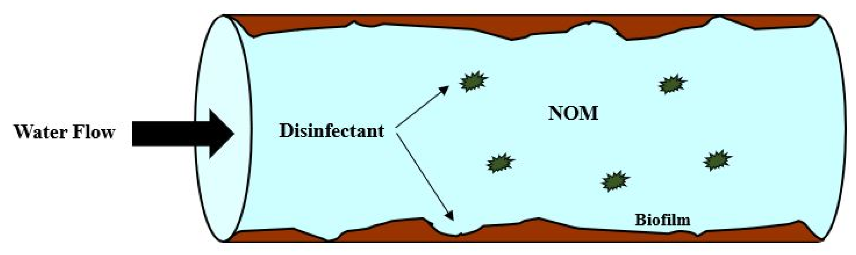
1.1. Water Quality in Water Distribution Networks
1.2. Measures against Low Residuals
1.3. Chlorine-Based Disinfectants
1.4. Disinfection Practices and Regulations
1.5. Aim of the Study
2. Materials and Methods
2.1. Methodology Adopted
2.1.1. Scenario 0—Chlorine
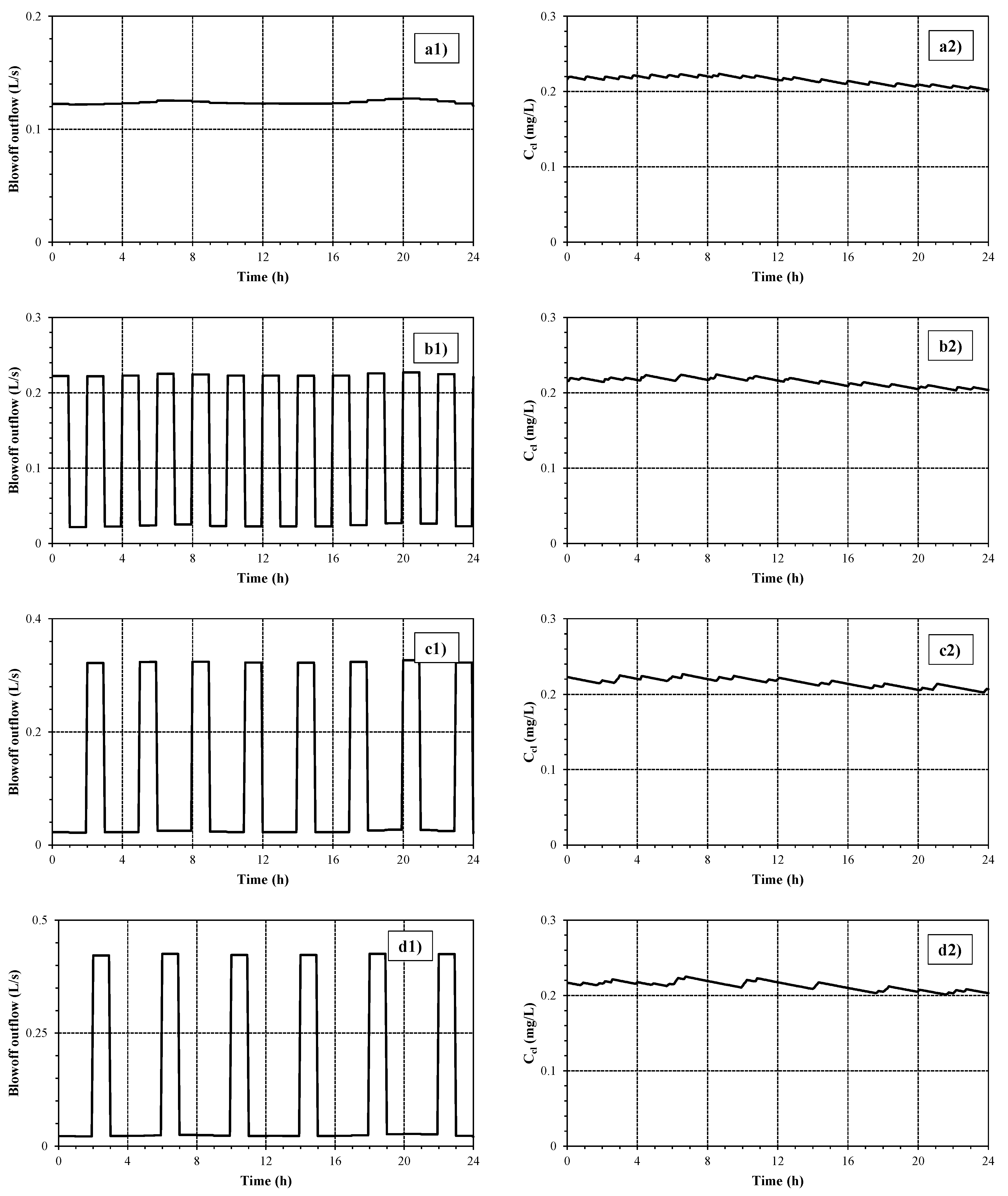
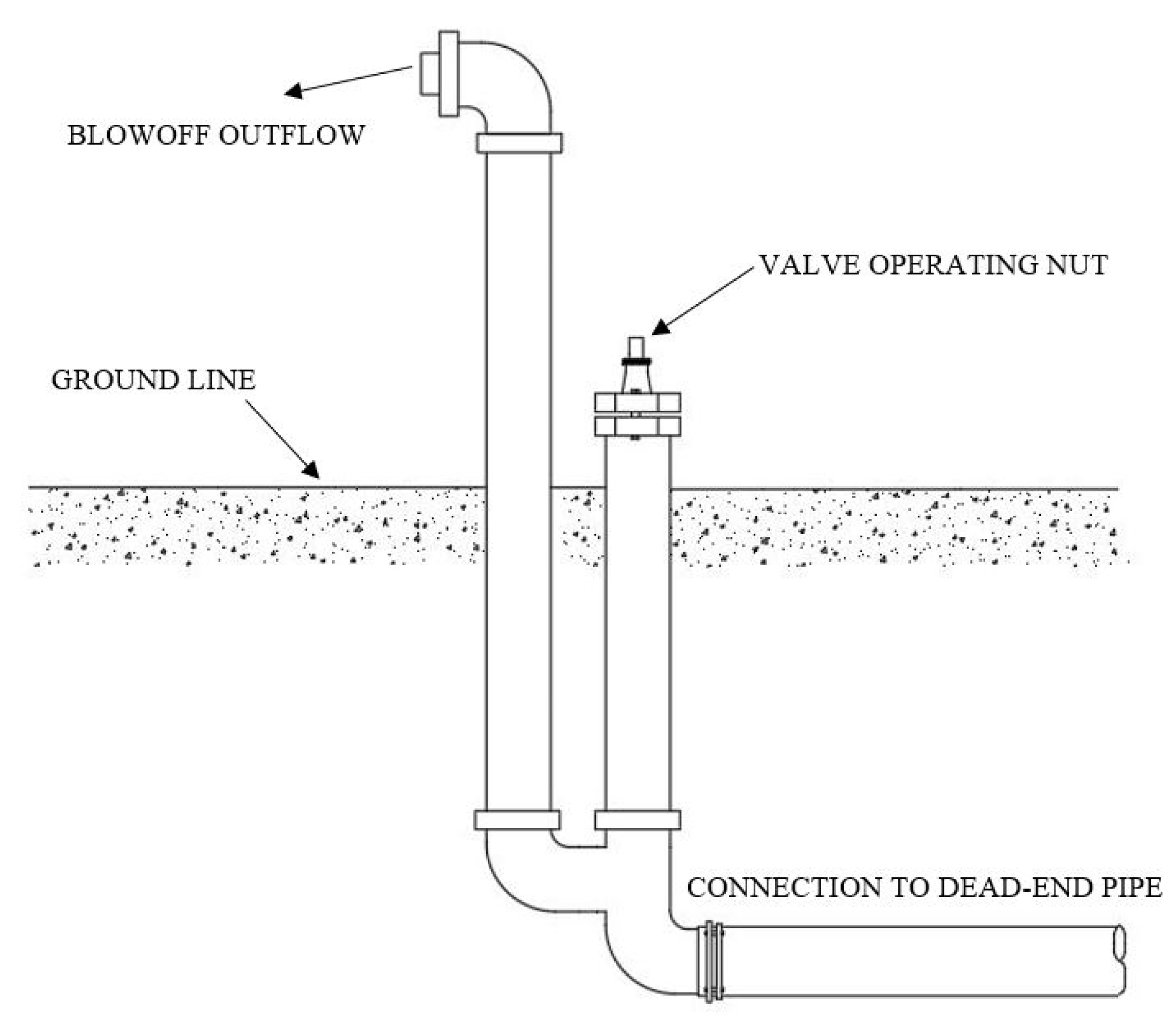
2.1.2. Scenario 1—Chlorine, Booster Stations, and Continuous Nodal Blowoffs
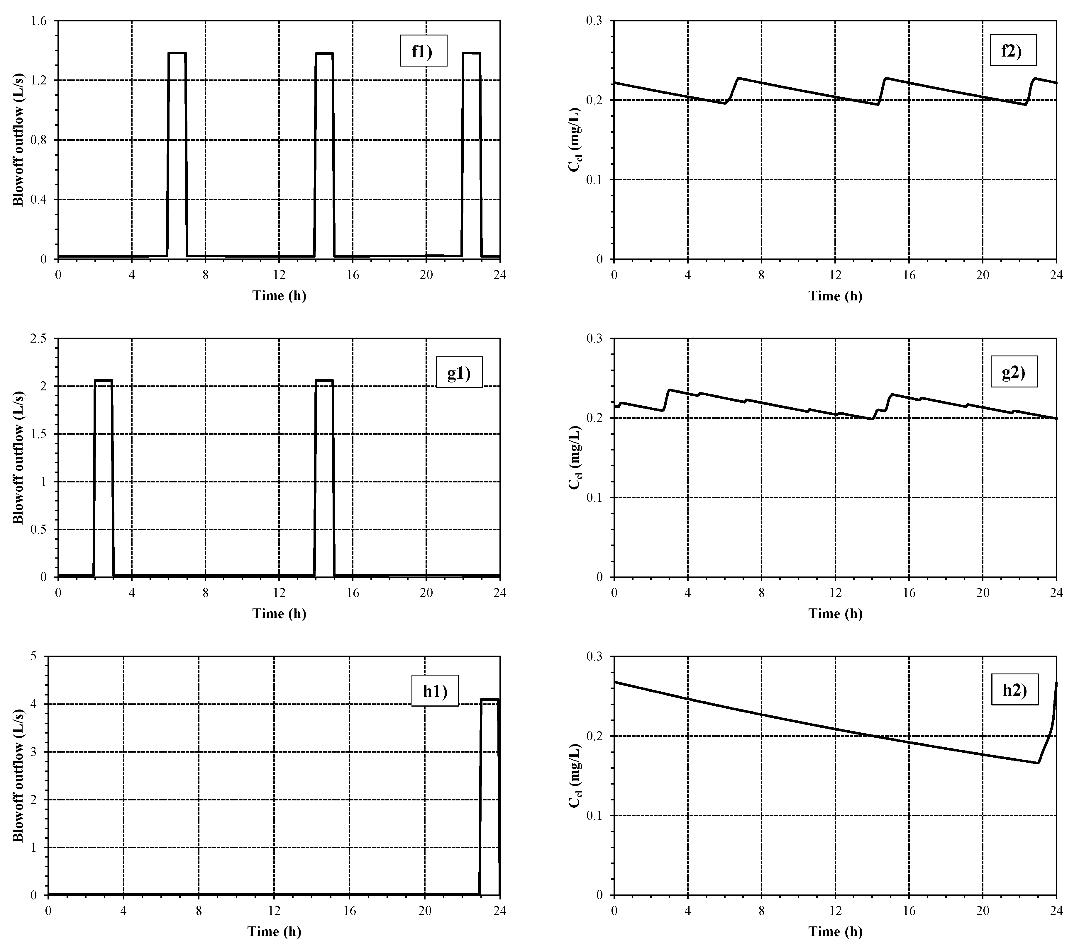
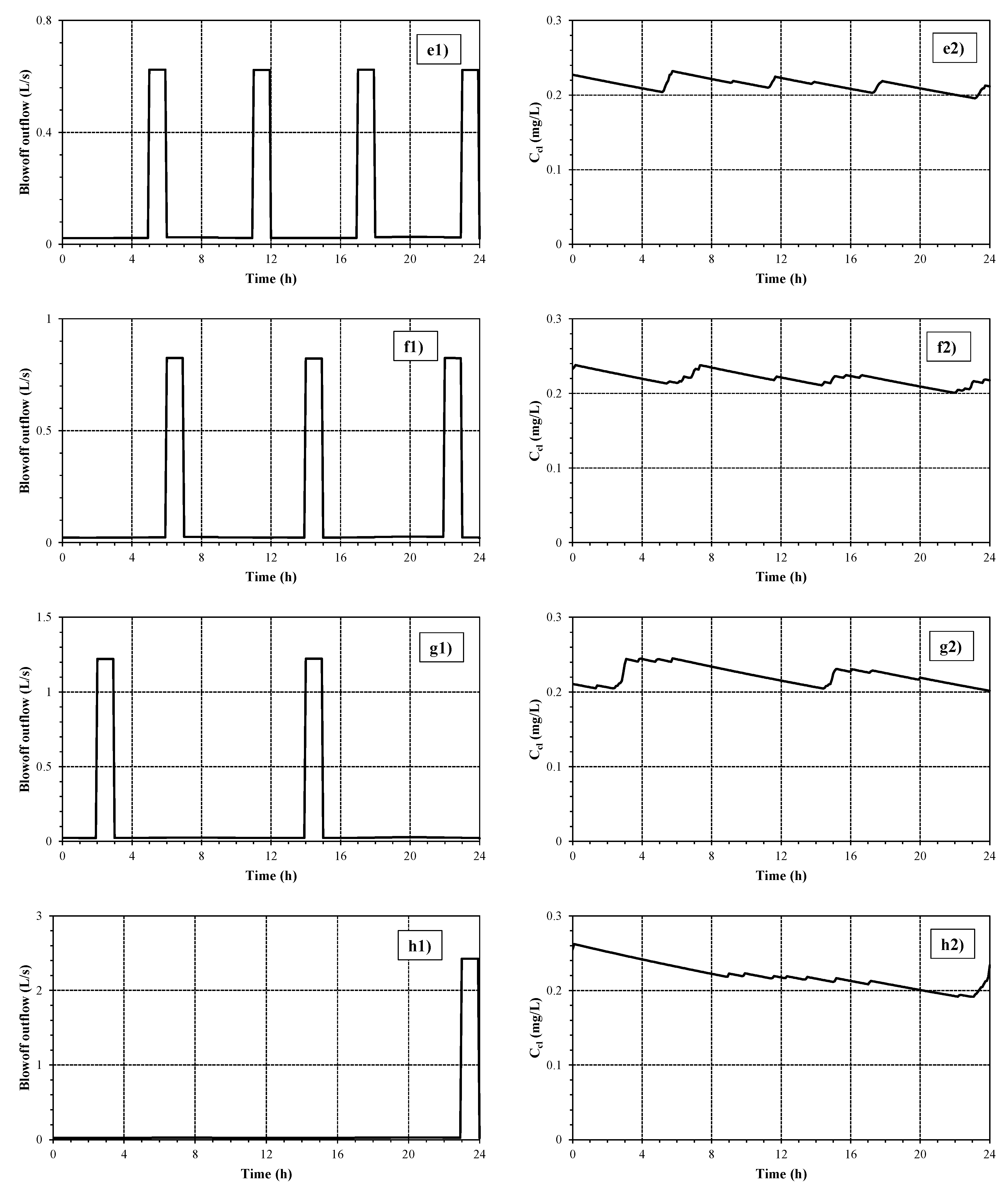
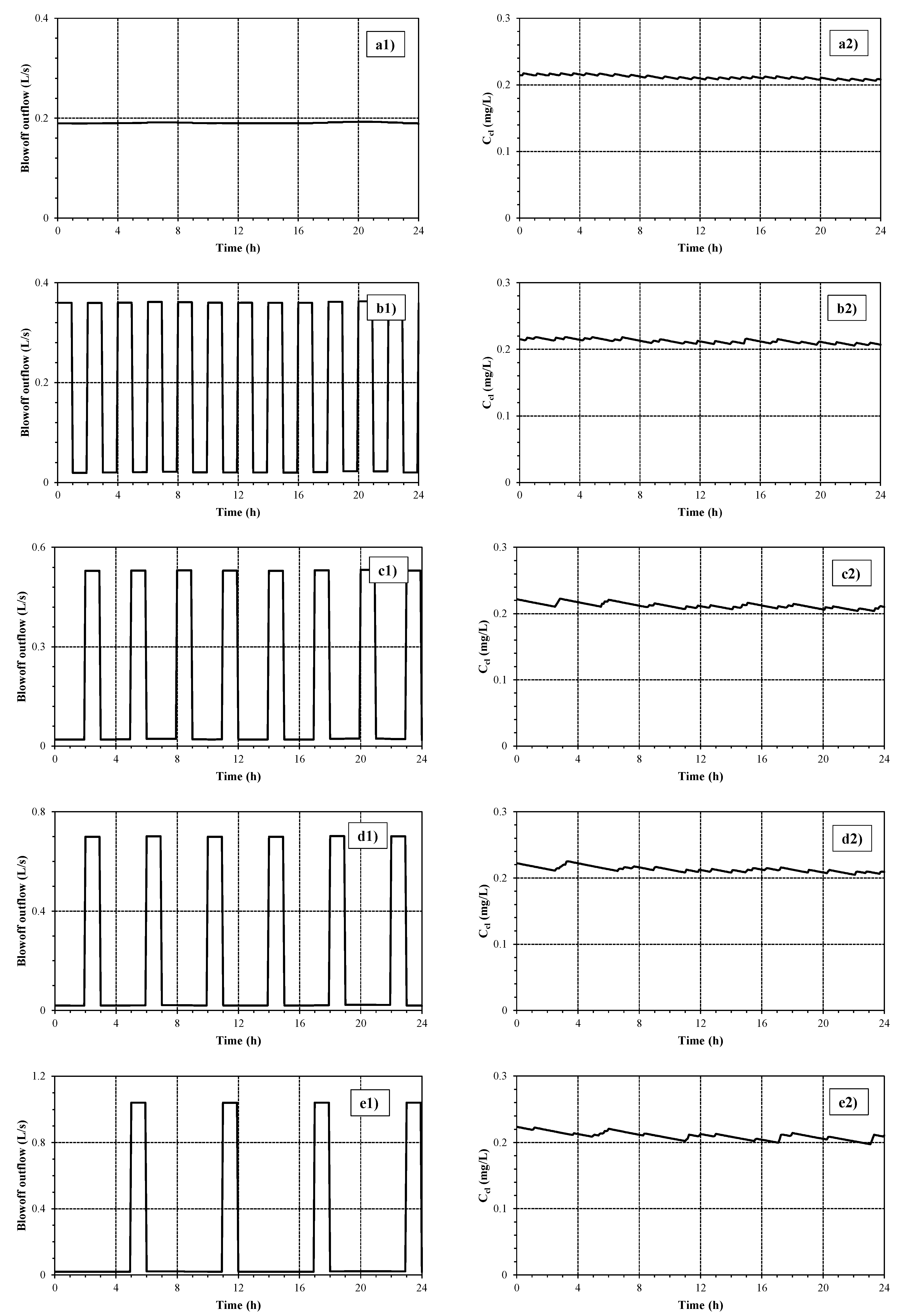
2.1.3. Scenario 2—Chlorine, Booster Stations, and Intermittent Nodal Blowoffs
2.1.4. Scenario 3—Chloramine
2.1.5. Scenario 4—Chloramine and Continuous Nodal Blowoffs
2.1.6. Estimation of Total Volume of Water and Total Mass of Disinfectant
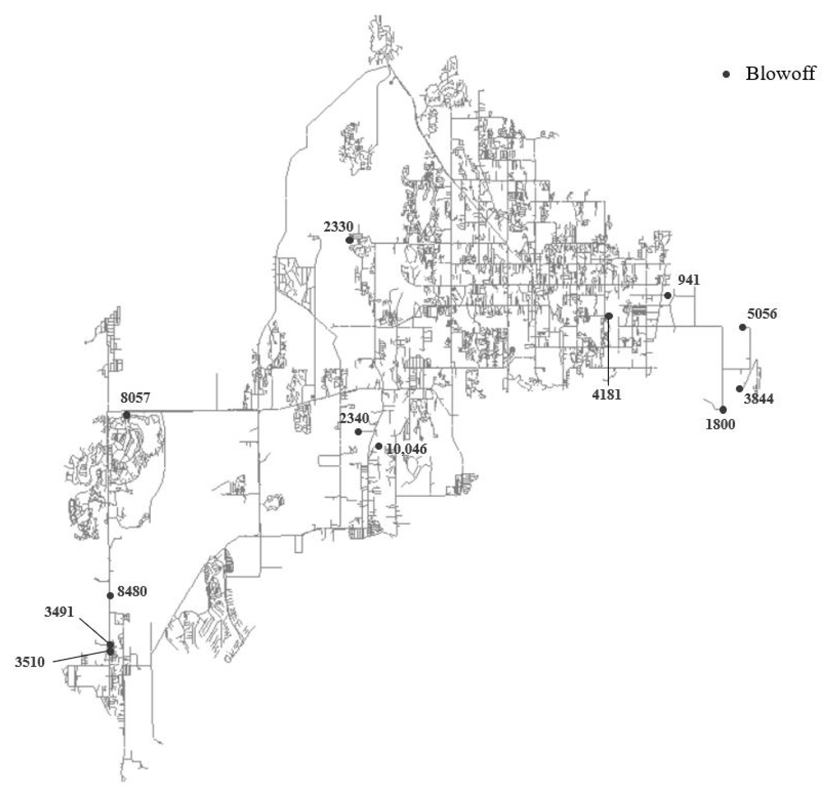
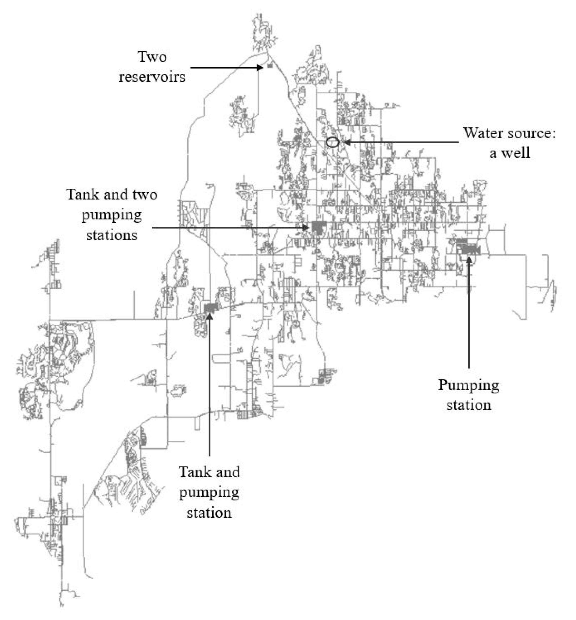
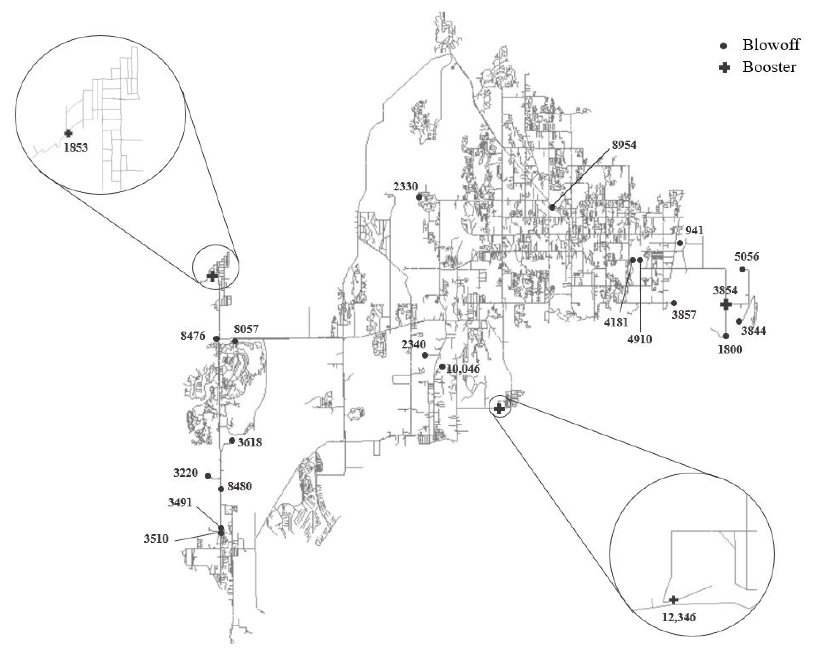
2.2. Case Study
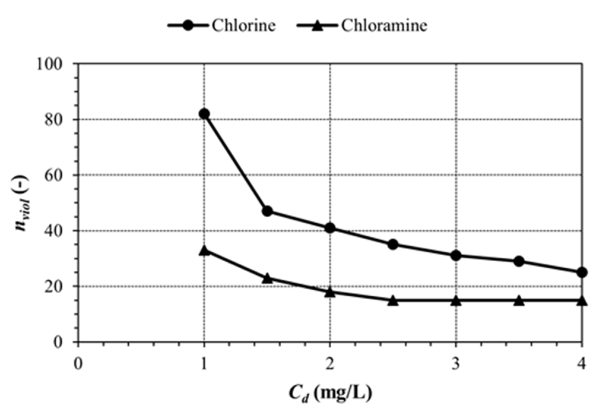
3. Results
4. Discussion
5. Conclusions
- -
- Booster stations are effective to obtain more uniform coverage of disinfectant and can be placed in suffering bulk areas, while nodal blowoffs seem to be a necessary solution for the numerous and scattered suffering dead-end nodes in WDN;
- -
- Intermittent blowoffs have a similar performance to the continuous blowoffs if a percentage of violation of 10–15% for a few hours per day is considered acceptable;
- -
- The use of chloramine as a possible alternative to chlorine led to an overall increase in residuals throughout the WDN and, consequently, to a decrease in the number of blowoffs to open and in blowoff outflows.
Author Contributions
Funding
Institutional Review Board Statement
Informed Consent Statement
Data Availability Statement
Conflicts of Interest
Appendix A

| Reaction Equation | Rate Coefficient |
|---|---|
| k1 = 0.5 d−1 a |
| N. | Reaction Stoichiometry | Rate Coefficient/Equilibrium Constant a |
|---|---|---|
| 1 | HOCl + NH3 → NH2Cl + H2O | k1 = 1.5 × 10¹⁰ M−1 h−1 |
| 2 | NH2Cl + H2O → HOCl + NH3 | k2 = 7.6 × 10⁻² h−1 |
| 3 | HOCl + NH2Cl → NHCl2 + H2O | k3 = 1.0 × 10⁶ M−1 h−1 |
| 4 | NHCl2 + H2O → HOCl + NH2Cl | k4 = 2.3 × 10⁻³ h−1 |
| 5 | NH2Cl + NH2Cl → NHCl2 + NH3 | k5 = 2.5 × 10⁷ [H+] + 4.0 × 10⁴ [H2CO3] + 800 [HCO3−] M−2 h−1 |
| 6 | NHCl2 + NH3 → NH2Cl + NH2Cl | k6 = 2.2 × 10⁸ M−2 h−1 |
| 7 | NHCl2 + H2O → I | k7 = 4.0 × 10⁵ M−1 h−1 |
| 8 | I + NHCl2 → HOCl + products | k8 = 1.0 × 10⁸ M−1 h−1 |
| 9 | I + NH2Cl → products | k9 = 3.0 × 10⁷ M−1 h−1 |
| 10 | NH2Cl + NHCL2 → products | k10 = 55.0 M−1 h−1 |
| 11 | NH2Cl + S1 b × TOC → products | k11 = 3.0 × 10⁴ M−1 h−1 S1 = 0.01 |
| 12 | HOCl + S2 c × TOC → products | k12 = 6.5 × 10⁵ M−1 h−1 S2 = 0.42 |
| 13 | HOCl ↔ H+ + OCl− | pKa1 = 7.5 |
| 14 | NH4+ ↔ NH3 + H+ | pKa2 = 9.3 |
| 15 | H2CO3 ↔ HCO3− + H+ | pKa3 = 6.3 |
| 16 | HCO3− ↔ CO32− + H+ | pKa4 = 10.3 |
References
- Decreto Legislativo 2 Febbraio 2001, n. 31. Attuazione Della Direttiva 98/83/CE Relativa Alla Qualità Delle Acque Destinate al Consumo Umano. Available online: https://www.gazzettaufficiale.it/eli/id/2001/03/03/001G0074/sg (accessed on 19 March 2022).
- National Water Quality Management Strategy. Australian Drinking-Water Guidelines 6; National Water Quality Management Strategy: Canberra, Australia, 2011. [Google Scholar]
- Health Canada. Guidelines for Canadian Drinking-Water Quality; Health Canada: Ottawa, ON, Canada, 2010. [Google Scholar]
- GB 5749-2006. Standards for Drinking-Water Quality. Available online: https://www.chinesestandard.net/PDF.aspx/GB5749-2006 (accessed on 19 March 2022).
- Safe Drinking Water Act (SDWA) 42 U.S.C. §300f et seq.(1974). Available online: https://www.epa.gov/laws-regulations/summary-safe-drinking-water-act (accessed on 19 March 2022).
- Vasconcelos, J.J.; Rossman, L.A.; Grayman, W.M.; Boulos, P.F.; Clark, R.M. Kinetics of chlorine decay. J. AWWA 1997, 89, 54–65. [Google Scholar] [CrossRef]
- Boccelli, D.L.; Tryby, M.E.; Uber, J.G.; Scott Summers, R. A reactive species model for chlorine decay and THM formation under rechlorination conditions. Water Res. 2003, 37, 2654–2666. [Google Scholar] [CrossRef]
- Zhu, N.; Mapili, K.; Majeed, H.; Pruden, A.; Edwards, M.A. Sediment and biofilm affect disinfectant decay rates during long-term operation of simulated reclaimed water distribution systems. Environ. Sci. Water Res. Technol. 2020, 6, 1615–1626. [Google Scholar] [CrossRef]
- Abokifa, A.A.; Jeffrey Yang, Y.; Lo, C.Y.; Biswas, P. Water quality modeling in the dead-end sections of drinking water distribution networks. Water Res. 2016, 89, 107–117. [Google Scholar] [CrossRef] [PubMed]
- World Health Organization (WHO). Guidelines for Drinking Water Quality, 4th ed.; Incorporating the 1st Addendum; WHO: Geneva, Switzerland, 2017. [Google Scholar]
- Walski, T.M. Raising the Bar on Disinfectant Residuals. World Water 2019, 42, 34–35. [Google Scholar]
- Li, X.-F.; Mitch, W.A. Drinkinq Water Disinfection Byproducts (DBPs) and Human Health Effects: Multidisciplinary Challenges and Opportunities. Environ. Sci. Technol. 2018, 52, 1681–1689. [Google Scholar] [CrossRef] [PubMed]
- Villanueva, C.M.; Cordier, S.; Font-Ribera, L.; Salas, L.A.; Levallois, P. Overview of Disinfection By-products and Associated Health Effects. Curr. Environ. Health Rep. 2015, 2, 107–115. [Google Scholar] [CrossRef] [PubMed] [Green Version]
- Tryby, M.E.; Bocelli, D.L.; Uber, J.G.; Rossman, L.A. Facility location model for booster disinfection of water supply networks. J. Water Resour. Plan. Manag. ASCE 2002, 128, 322–333. [Google Scholar] [CrossRef]
- Bocelli, D.L.; Tryby, M.E.; Uber, J.G.; Rossman, L.A.; Zierolf, M.L.; Polycarpou, M. Optimal scheduling of booster disinfection in water distribution systems. J. Water Resour. Plan. Manag. ASCE 1998, 124, 99–111. [Google Scholar] [CrossRef]
- Prasad, T.D.; Walters, G.A.; Savic, D.A. Booster disinfection of water supply networks: Multi objective approach. J. Water Resour. Plan. Manag. ASCE 2004, 130, 367–376. [Google Scholar] [CrossRef]
- Lansey, K.; Pasha, F.; Pool, S.; Elshorbagy, W.; Uber, J. Locating satellite booster disinfectant stations. J. Water Resour. Plan. Manag. ASCE 2007, 133, 372–376. [Google Scholar] [CrossRef]
- Meng, F.; Liu, S.; Ostfeld, A.; Chen, C.; Burchard-Levine, A. A deterministic approach for optimization of booster disinfection placement and operation for a water distribution system in Beijing. J. Hydroinform. 2013, 15, 1042–1058. [Google Scholar] [CrossRef] [Green Version]
- Goyal, R.V.; Patel, H.M. Optimal location and scheduling of booster chlorination stations using EPANET and PSO for drinking water distribution system. ISH J. Hydraul. Eng. 2018, 24, 157–164. [Google Scholar] [CrossRef]
- Kang, D.; Lansey, K. Real-Time Optimal Valve Operation and Booster Disinfection for Water Quality in Water Distribution Systems. J. Water Resour. Plan. Manag. ASCE 2010, 136, 463–473. [Google Scholar] [CrossRef]
- Ohar, Z.; Ostfeld, A. Optimal design and operation of booster chlorination stations layout in water distribution systems. Water Res. 2014, 58, 209–220. [Google Scholar] [CrossRef]
- Hubbs, S. Flush with Success: Water Mains and Fire Hydrants. Water Quality & Health Council. 2020. Available online: www.waterandhealth.org (accessed on 19 March 2022).
- Friedman, M.J.; Martel, K.; Hill, A.; Holt, D.; Smith, S.; Ta, T.; Sherwin, C.; Hiltebrand, D.; Pommerenk, P.; Hinedi, Z.; et al. Establishing Site Specific Flushing Velocities. In Proceedings of the AWWA and AwwaRF Conference, Denver, CO, USA, 1 June 2003. [Google Scholar]
- Antoun, E.N.; Tyson, T.; Hiltebrand, D. Unidirectional flushing: A remedy to water quality problems such as biologically mediated corrosion. In Proceedings of the AWWA Annual Conference, Denver, CO, USA, 1 June 1997. [Google Scholar]
- Friedman, M.; Kirmeyer, G.J.; Antoun, E. Developing and implementing a distribution system flushing program. J. AWWA 2002, 94, 48–56. [Google Scholar] [CrossRef]
- Barbeau, B.; Gauthier, V.; Julienne, K.; Carriere, A. Dead-end flushing of a distribution system: Short and long-term effects on water quality. J. Water Supply Res. Technol.-AQUA 2005, 54, 371–383. [Google Scholar] [CrossRef]
- Carrière, A.; Gauthier, V.; Desjardins, V.; Barbeau, B. Evaluation of loose deposits in distribution systems through unidirectional flushing. J. AWWA 2005, 97, 82–92. [Google Scholar] [CrossRef]
- Deuerlein, J.; Simpson, A.R.; Korth, A. Flushing planner: A tool for planning and optimization of unidirectional flushing. 12th International Conference on Computing and Control for the Water Industry, CCWI2013. Proceedia Eng. 2014, 70, 497–506. [Google Scholar] [CrossRef] [Green Version]
- Baranowski, T.M.; Walski, T.M. Modeling a hydraulic response to a contamination event. In World Environmental and Water Resources Congress: Great Rivers; Environment and Water Resources Institute: Kansas City, MO, USA, 2009. [Google Scholar]
- Poulin, A.; Mailhot, A.; Periche, N.; Delorme, L.; Villeneuve, J.-P. Planning Unidirectional Flushing Operations as a response to Drinking Water Distribution System Contamination. J. Water Resour. Plan. Manag. ASCE 2010, 136, 647–657. [Google Scholar] [CrossRef] [Green Version]
- Walski, T.M.; Draus, S. Predicting Water Quality Changes during Flushing. In American Water Works Association Annual Conference; American Water Works Association: Denver, CO, USA, 1996. [Google Scholar]
- Xie, X.; Nachabe, M.; Zeng, B. Optimal Scheduling of Automatic Flushing Devices in Water Distribution System. J. Water Resour. Plan. Manag. ASCE 2014, 141, 04014081. [Google Scholar] [CrossRef]
- Avvedimento, S.; Todeschini, S.; Giudicianni, C.; Di Nardo, A.; Walski, T.; Creaco, E. Modulating nodal outflows to guarantee sufficient disinfectant residuals in water distribution networks. J. Water Resour. Plan. Manag. ASCE 2020, 146, 04020066. [Google Scholar] [CrossRef]
- Zhang, Q.; Davies, E.G.R.; Bolton, J.; Liu, Y. Monochloramine loss mechanisms in tap water. Water Environ. Res. 2017, 89, 1999–2005. [Google Scholar] [CrossRef] [PubMed]
- Duirk, S.E.; Valentine, R.L. Bromide oxidation and formation of dihaloacetic acids in chloraminated water. Environ. Sci. Technol. 2007, 41, 7047–7053. [Google Scholar] [CrossRef] [PubMed]
- Kadwa, U.; Kumarasamy, M.V.; Stretch, D. Effect of chlorine and chloramine disinfection and the presence of phosphorous and nitrogen on biofilm growth in dead zones on PVC pipes in drinking water systems. J. S. Afr. Inst. Civ. Eng. 2018, 60, 45–50. [Google Scholar] [CrossRef]
- Agudelo-Vera, C.; Avvedimento, S.; Boxall, J.; Creaco, E.; de Kater, H.; Di Nardo, A.; Djukic, A.; Douterelo, I.; Fish, K.E.; Iglesias Rey, P.L.; et al. Drinking Water Temperature around the Globe: Understanding, Policies, Challenges and Opportunities. Water 2020, 12, 1049. [Google Scholar] [CrossRef] [Green Version]
- LeChevallier, M.W.; Au, K.-K.; World Health Organization. Water Treatment and Pathogen Control: Process Efficiency in Achieving Safe Drinking Water; World Health Organization: Geneva, Switzerland, 2004. [Google Scholar]
- CDC (Centeres for Disease Control and Prevention). Effect of Chlorination on Inactivating Selected Pathogen. Available online: https://www.cdc.gov/healthywater/global/household-water-treatment/effectiveness-on-pathogens.html (accessed on 19 March 2022).
- U.S. Enviromental Protection Agency. The Effectiveness of Disinfectant Residuals in the Distribution System; U.S. Enviromental Protection Agency: Washington, DC, USA, 2007.
- Kirmeyer, G.J.; Foust, G.W.; Pierson, G.L.; Simmler, J.J.; LeChevallier, M.W. Optimizing Chloramine Treatment; American Water Works Association: Denver, CO, USA, 1993. [Google Scholar]
- U.S. Environmental Protection Agency. Chloramines in Drinking Water; U.S. Enviromental Protection Agency: Washington, DC, USA, 2012.
- Kirmeyer, G.J.; Martel, K.; Thompson, G.; Radder, L.; Klement, W.; LeChevallier, M.; Flores, A. Optimizing chloramine treatment. In Proceedings of the AWWA Conference, Denver, CO, USA, 1 June 2004. [Google Scholar]
- Vikesland, P.J.; Ozekin, K.; Valentine, R.L. Monochloramine decay in model and distribution system waters. Water Res. 2001, 35, 1766–1776. [Google Scholar] [CrossRef]
- Duirk, S.E.; Gombert, B.; Croue, J.-P.; Valentine, R.L. Modeling monochloramine loss in the presence of natural organic matter. Water Res. 2005, 39, 3418–3431. [Google Scholar] [CrossRef]
- Fisher, I.; Kastl, G.; Fayle, B.; Sathasivan, A. Chlorine or chloramine for drinking water disinfection? Water 2009, 36, 52–62. [Google Scholar]
- Alexander, M.T.; Boccelli, D.L. Field verification of an integrated hydraulic and multi-species water quality model. In Proceedings of the Water Distribution Systems Analysis 2010—12th International Conference WDSA, Tucson, AZ, USA, 12–15 September 2010; pp. 687–696. [Google Scholar]
- Ricca, H.; Aravinthan, V.; Mahinthakumar, G. Modeling chloramine decay in full-scale drinking water supply systems. Water Environ. Res. 2019, 91, 441–454. [Google Scholar] [CrossRef]
- Wilczak, A.; Jacangelo, J.G.; Marcinko, J.P.; Odell, L.H.; Kirmeyer, G.J.; Wolfe, R.L. Occurrence of nitrification in chloraminated distribution systems. J. AWWA 1996, 88, 74–85. [Google Scholar] [CrossRef]
- Zhang, Y.; Triantafyllidou, S.; Edwards, M. Effect of nitrification and GAC filtration on copper and lead leaching in home plumbing systems. J. Environ. Eng. 2008, 134, 521–530. [Google Scholar] [CrossRef]
- Rosario-Ortiz, F.; Rose, J.; Speight, V.; von Gunten, U.; Schnoor, J. How do you like your tap water? Science 2016, 351, 912–914. [Google Scholar] [CrossRef] [PubMed]
- Health Canada. Chloramines in Drinking Water Guideline Technical Document for Public Consultation; Health Canada: Ottawa, ON, Canada, 2018. [Google Scholar]
- Rossman, L.; Woo, H.; Tryby, M.; Shang, F.; Janke, R.; Haxton, T. EPANET 2.2 User Manual; U.S. Environmental Protection Agency: Washington, DC, USA, 2020.
- Propato, M.; Uber, J.G. Vulnerability of Water Distribution Systems to Pathogen Intrusion: How Effective is a Disinfectant Residual? Environ. Sci. Technol. 2004, 38, 3713–3722. [Google Scholar] [CrossRef] [PubMed]
- Shang, F.; Uber, J.; Rossman, L.A. EPANET Multi-Species Extension USER’S manual; Rep. No. EPA/600/S-07/021; USEPA: Cincinnati, NO, USA, 2008. [Google Scholar]
- MATLAB 2021a; The MathWorks, Inc.: Natick, MA, USA, 2021.
- Rossman, L.A.; Clark, R.M.; Grayman, W.M. Modeling chlorine residuals in drinking water distribution systems. J. Environ. Eng. ASCE 1994, 120, 803–820. [Google Scholar] [CrossRef]
- Powell, J.C.; Hallam, N.B.; West, J.R.; Forster, C.F.; Simms, J. Factors which control bulk chlorine decay rates. Water Res. 2000, 34, 117–126. [Google Scholar] [CrossRef]
- Nejjari, F.; Puig, V.; Pérez, R.; Quevedo, J.; Cugueró, M.A.; Sanz, G.; Mirats, J.M. Chlorine decay model calibration and comparison: Application to a real water network. In Proceedings of the 2013 12th International Conference on Computing and Control for the Water Industry, CCWI2013, Perugia, Italy, 2–4 September 2013. [Google Scholar]
- APAT (Agenzia per la Protezione dell’Ambiente e per i servizi Tecnici); IRSA-CNR (Istituto di Ricerca sulle Acque-Consiglio Nazionale delle Ricerche). Metodi Analitici per le Acque; APAT: Rome, Italy, 2004; pp. 645–651. ISBN 88-448-0083-7. [Google Scholar]
- Ostfeld, A.; Uber, J.G.; Salomons, E.; Berry, J.W.; Hart, W.E.; Phillips, C.A.; Watson, J.P.; Dorini, G.; Jonkergouw, P.; Kapelan, Z.; et al. The Battle of the Water Sensor Networks (BWSN): A Design Challenge for Engineers and Algorithms. J. Water Resour. Plan. Manag. ASCE 2008, 134, 556–568. [Google Scholar] [CrossRef] [Green Version]
- Council Directive 98/83/EC of 3 November 1998 on the Quality of Water Intended for Human Consumption. Available online: https://eur-lex.europa.eu/legal-content/EN/ALL/?uri=CELEX:31998L0083 (accessed on 11 January 2022).


| Scenario | Disinfectant | N. of Booster Station | Flushing Blowoffs | N. of Violating Nodes |
|---|---|---|---|---|
| 0 | Chlorine | 0 | 0 | 41 |
| 1 | Chlorine | 3 | 18-continuous | 0 |
| 2 | Chlorine | 3 | 18-intermittent | 0 |
| 3 | Chloramine | 0 | 0 | 18 |
| 4 | Chloramine | 0 | 12-continuous | 0 |
| Node | e (L/s/m1/2) | q (L/s) | e (L/s/m1/2) | q (L/s) |
|---|---|---|---|---|
| ID | Scenario 1 | Scenario 1 | Scenario 4 | Scenario 4 |
| 941 | 0.0052 | 0.033 | 0.003 | 0.019 |
| 1800 | 0.026 | 0.192 | 0.023 | 0.170 |
| 2330 | 0.0081 | 0.056 | 0.0025 | 0.018 |
| 2340 | 0.013 | 0.117 | 0.0046 | 0.054 |
| 3220 | 0.0024 | 0.071 | - | - |
| 3491 | 0.016 | 0.154 | 0.0064 | 0.078 |
| 3510 | 0.015 | 0.127 | 0.0069 | 0.062 |
| 3844 | 0.016 | 0.124 | 0.014 | 0.109 |
| 3618 | 0.0068 | 0.081 | - | - |
| 3857 | 0.0033 | 0.027 | - | - |
| 4181 | 0.005 | 0.046 | 0.0025 | 0.028 |
| 4910 | 0.0038 | 0.032 | - | |
| 5056 | 0.038 | 0.238 | 0.033 | 0.208 |
| 8057 | 0.028 | 0.228 | 0.013 | 0.121 |
| 8480 | 0.042 | 0.352 | 0.018 | 0.175 |
| 8476 | 0.0032 | 0.149 | - | - |
| 8954 | 0.0028 | 0.029 | - | - |
| 10046 | 0.041 | 0.381 | 0.014 | 0.169 |
| Sub Scenario | k Hours of Blowoff in the Day | Blowoff Flow q1800,k (L/s) | First Hour j of Outflow in the Day (h) | Duration vk,j of Violations (min) |
|---|---|---|---|---|
| 2a | 24 | 0.17 | 1 (from 0 h to 1 h) | 0 |
| 2b | 12 | 0.34 | 1 (from 0 h to 1 h) | 0 |
| 2c | 8 | 0.51 | 3 (from 2 h to 3 h) | 0 |
| 2d | 6 | 0.68 | 3 (from 2 h to 3 h) | 0 |
| 2e | 4 | 1.02 | 6 (from 5 h to 6 h) | 0 |
| 2f | 3 | 1.36 | 7 (from 6 h to 7 h) | 150 |
| 2g | 2 | 2.04 | 3 (from 2 h to 3 h) | 0 |
| 2h | 1 | 4.08 | 24 (from 23 h to 24 h) | 515 |
| Sub Scenario | k Hours of Blowoff in the Day | Blowoff Flow q3510,k (L/s) | First Hour j of Outflow in the Day (h) | Duration vk,j of Violations (min) |
|---|---|---|---|---|
| 2a | 24 | 0.1 | 1 (from 0 h to 1 h) | 0 |
| 2b | 12 | 0.2 | 1 (from 0 h to 1 h) | 0 |
| 2c | 8 | 0.3 | 3 (from 2 h to 3 h) | 0 |
| 2d | 6 | 0.4 | 3 (from 2 h to 3 h) | 0 |
| 2e | 4 | 0.6 | 6 (from 5 h to 6 h) | 40 |
| 2f | 3 | 0.8 | 7 (from 6 h to 7 h) | 0 |
| 2g | 2 | 1.2 | 3 (from 2 h to 3 h) | 0 |
| 2h | 1 | 2.4 | 24 (from 23 h to 24 h) | 155 |
| Scenario | W (kg) | Vol (m3) |
|---|---|---|
| 0 | 3171 | 1,585,416 |
| 1 | 3174 | 1,586,871 |
| 4 | 3172 | 1,586,177 |
Publisher’s Note: MDPI stays neutral with regard to jurisdictional claims in published maps and institutional affiliations. |
© 2022 by the authors. Licensee MDPI, Basel, Switzerland. This article is an open access article distributed under the terms and conditions of the Creative Commons Attribution (CC BY) license (https://creativecommons.org/licenses/by/4.0/).
Share and Cite
Avvedimento, S.; Todeschini, S.; Manenti, S.; Creaco, E. Comparison of Techniques for Maintaining Adequate Disinfectant Residuals in a Full-Scale Water Distribution Network. Water 2022, 14, 1029. https://doi.org/10.3390/w14071029
Avvedimento S, Todeschini S, Manenti S, Creaco E. Comparison of Techniques for Maintaining Adequate Disinfectant Residuals in a Full-Scale Water Distribution Network. Water. 2022; 14(7):1029. https://doi.org/10.3390/w14071029
Chicago/Turabian StyleAvvedimento, Stefania, Sara Todeschini, Sauro Manenti, and Enrico Creaco. 2022. "Comparison of Techniques for Maintaining Adequate Disinfectant Residuals in a Full-Scale Water Distribution Network" Water 14, no. 7: 1029. https://doi.org/10.3390/w14071029
APA StyleAvvedimento, S., Todeschini, S., Manenti, S., & Creaco, E. (2022). Comparison of Techniques for Maintaining Adequate Disinfectant Residuals in a Full-Scale Water Distribution Network. Water, 14(7), 1029. https://doi.org/10.3390/w14071029