Foraminiferal Distribution in Two Estuarine Intertidal Mudflats of the French Atlantic Coast: Testing the Marine Influence Index

Abstract

This study focuses on the foraminiferal distribution on intertidal mudflats of two contrasted estuaries (Auray and Vie) along the French Atlantic coast. In both estuaries, the foraminiferal communities are dominated by Haynesina germanica and the Ammonia tepida group. Stations located near the outlets show a high diversity and abundance of species of the genus Elphidium. Stations in the inner estuary show a higher proportion of agglutinated species (Ammotium salsum, Ammobaculites agglutinans). Multivariate statistical analysis suggests that the distance to the sea and the percentage of fine sediment (<63 µm) are the two main parameters explaining the foraminiferal distribution. Chemical analyses of the sediment show that the two studied estuaries are not affected by major anthropogenic pollution, so that the faunas should mainly reflect the natural controlling parameters. Three indices of environmental quality commonly used in coastal areas show counter-intuitive differences between stations, suggesting that these indices may be less reliable for use in intertidal estuarine mudflats. The newly developed Marine Influence Index (MII) integrates three major ecological factors: the position of the sampling point on the salinity gradient, the emergence time at low tide and the relative importance of fresh water discharge. In our dataset, MII shows significant correlations with the controlling environmental parameters (distance to the sea, percentage grains < 63 µm), as well as with the foraminiferal patterns (PCA axis 1, species richness, percentage of Elphidium spp. and Quinqueloculina spp.). These results suggest that the MII explains a substantial part of the faunal variability on estuarine intertidal mudflats, and can be used to detect deviations from the natural distribution patterns in response to anthropogenic pollution.

1. Introduction

Whitfield and Elliott [1] defined estuaries as “semi-enclosed coastal water bodies connected to the sea either permanently or periodically, having a different salinity compared to the adjacent open ocean due to freshwater inputs, and being inhabited by a characteristic biota”. Estuaries are among the most dynamic ecosystems of the marine realm [2]. They host productive transitional water ecosystems of high ecological and economic interest [3]. Estuaries are buffer zones protecting coastal plains against climatic events (i.e., storms, floods), and are important nursery habitats for fish and other migratory animals [2,4]. They are also suitable locations for human settlement due to their ideal geographical situation at the interface between continents and oceans. For centuries, they have been subjected to anthropogenic disturbances, stress and habitat modifications, because they host multiple economic activities (e.g., fishery, aquaculture, tourism, industry, urbanisation) [5,6,7]. In this context, the European community has established the Water Framework Directive [8], requesting member countries to monitor the environmental quality of various water bodies (including transitional systems such as estuaries), and when necessary, to take measures to return to a good water quality status.

Over the last few decades, the use of biotic indices to assess the environmental quality of coastal waters has expanded considerably. Several groups of organisms are used as bioindicators (e.g., fish, algae, benthic macrofauna and meiofauna) because of their sensitivity to natural and anthropogenic disturbance [9]. Among these, foraminifera (Eukaryotes, Rhizaria) have several advantages: (1) they have a sedentary lifestyle, (2) they have short life cycles (up to 2 years) that ensure a rapid response to environmental change [10,11], (3) they inhabit almost all marine regions and transitional waters [10], (4) they show high species diversity (about 9000 living species) with a large panel of functional traits [12], and (5) their fossil records can be analysed to gain insight into their community composition before recent anthropogenic impacts, and thereby can provide pristine reference conditions [13,14].

Recently, several studies have developed foraminiferal biotic indices for coastal areas. Some of these indices are based on alpha diversity (e.g., [15]), whereas others apply an indicator species concept, using the relative proportion of stress-tolerant species (e.g., [14,16,17,18,19]). These species are often recognised as such by their response to organic matter enrichment in the sediment. However, in estuarine environments, both the spatial and the temporal variation in physical and chemical parameters are very high (e.g., salinity, temperature, water movement, turbidity, oxygen content, organic matter supplies, etc.). Such a strong variability induces natural stress that affects local biota. Consequently, estuaries show a low biodiversity, with a dominance of species adapted to adverse conditions. Even pristine estuarine communities are dominated by stress-tolerant species that are adapted to highly fluctuating environmental conditions, leading to low values for most indices of environmental quality. This observation has been named the “estuarine paradox” [20,21]. Consequently, the development of biotic indices for the highly complex and dynamic ecosystems found in estuaries is a real challenge [22,23].

Due to the “estuarine paradox”, foraminiferal bio-indication indices developed in open marine environments cannot be applied directly to estuaries. Several strategies have been proposed to overcome this difficulty. Bouchet et al. [24] proposed to use the corrected Shannon diversity index Exp(H’bc) in Mediterranean transitional zones and adapted the ecological class boundaries to this particular environment. More recently, Bouchet et al. [25] proposed a list of stress-tolerant species, based on their response to organic matter gradients occurring in transitional waters.

In principle, the construction of a foraminiferal index of environmental quality in estuaries requires prior knowledge of their natural distribution. Only once this natural distribution, and the relation with the controlling parameters, is fully understood can it become possible to recognise distributional anomalies resulting from anthropogenic stress. However, at present, most estuaries are impacted by both natural and anthropogenic stresses. There is a general scientific consensus that the main natural parameter influencing the distribution of foraminifera in estuarine environments is salinity (e.g., [26,27,28,29]). Estuaries are characterised by strong daily and seasonal salinity variations. The daily aerial exposure due to the tidal cycle (twice a day in the studied area) is an additional natural stress factor for the foraminiferal communities on estuarine intertidal flats. This leads to high temperature and salinity variations due to evaporation/precipitation at low tide, and a mix of marine and fresh waters at high tide [29,30,31]. Other main controlling parameters are sediment grain size and natural organic matter quantity and quality [32,33].

When superposed on these natural parameters, anthropogenic stress can modify the distribution of benthic foraminifera. For instance, high concentrations in trace metals can influence the density, species richness and composition of communities, and can lead to an increase in abnormal tests [34,35,36]. An excess of anthropogenic organic matter (e.g., domestic sewage, or estuarine primary production resulting from fertiliser input) can also modify the community composition [34,37]. Moreover, inputs of large quantities of organic matter may induce hypoxic or anoxic zones, where oxygen consumption exceeds supply. Such events intensify during warm late summer and early autumn months [38]. Other anthropogenic pollutants (e.g., hydrocarbons, hormones) and anthropogenic physical disturbance can impact living communities as well [39].

In an attempt to integrate the main natural factors affecting estuarine foraminifera in a single environmental index, Jorissen et al. (this volume) [40] proposed the Marine Influence Index (MII). The MII, calculated for each sampling station, is based on the position of the studied station along the salinity gradient, the duration of tidal emergence and the relative importance of river runoff in the ambient water turnover. Therefore, this index reflects salinity, but implicitly also the hydrodynamic energy and fluviatile and/or marine particle supplies.

The first aim of the present study is to assess the foraminiferal distribution (of the >125 µm fraction) living in the surficial sediment of intertidal mudflats along two contrasted estuaries of the French Atlantic coast. The main parameters controlling the foraminiferal communities in these environments will be identified. Next, we will investigate whether at one or more stations, the foraminiferal composition deviates from the composition expected under natural conditions, and whether this deviation is due to anthropogenic pollution. Some foraminiferal indices of environmental quality commonly used in transitional waters will be applied and assessed for their applicability to intertidal estuarine mudflats. Finally, we will investigate to what extent MII, which describes the marine influence in estuaries, is correlated with the characteristics of the foraminiferal communities, and can be used to detect distributional anomalies due to anthropogenic pollution.

2. Material and Methods

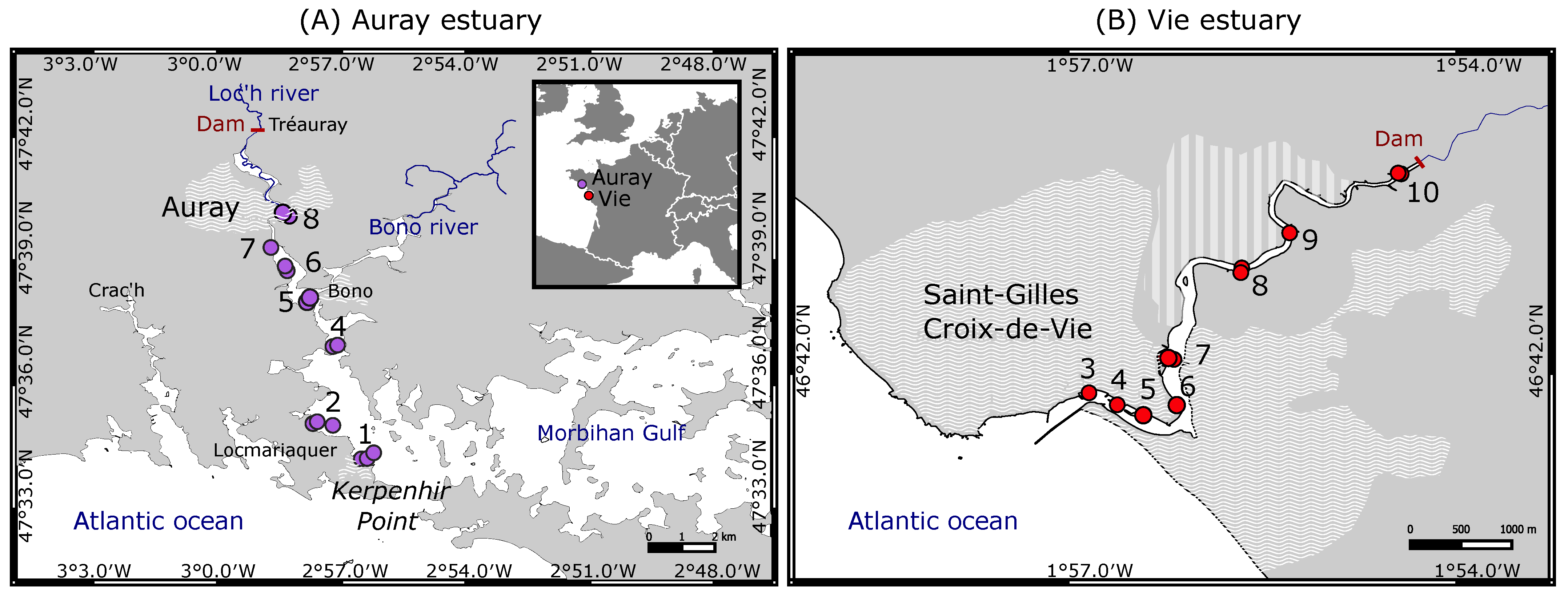
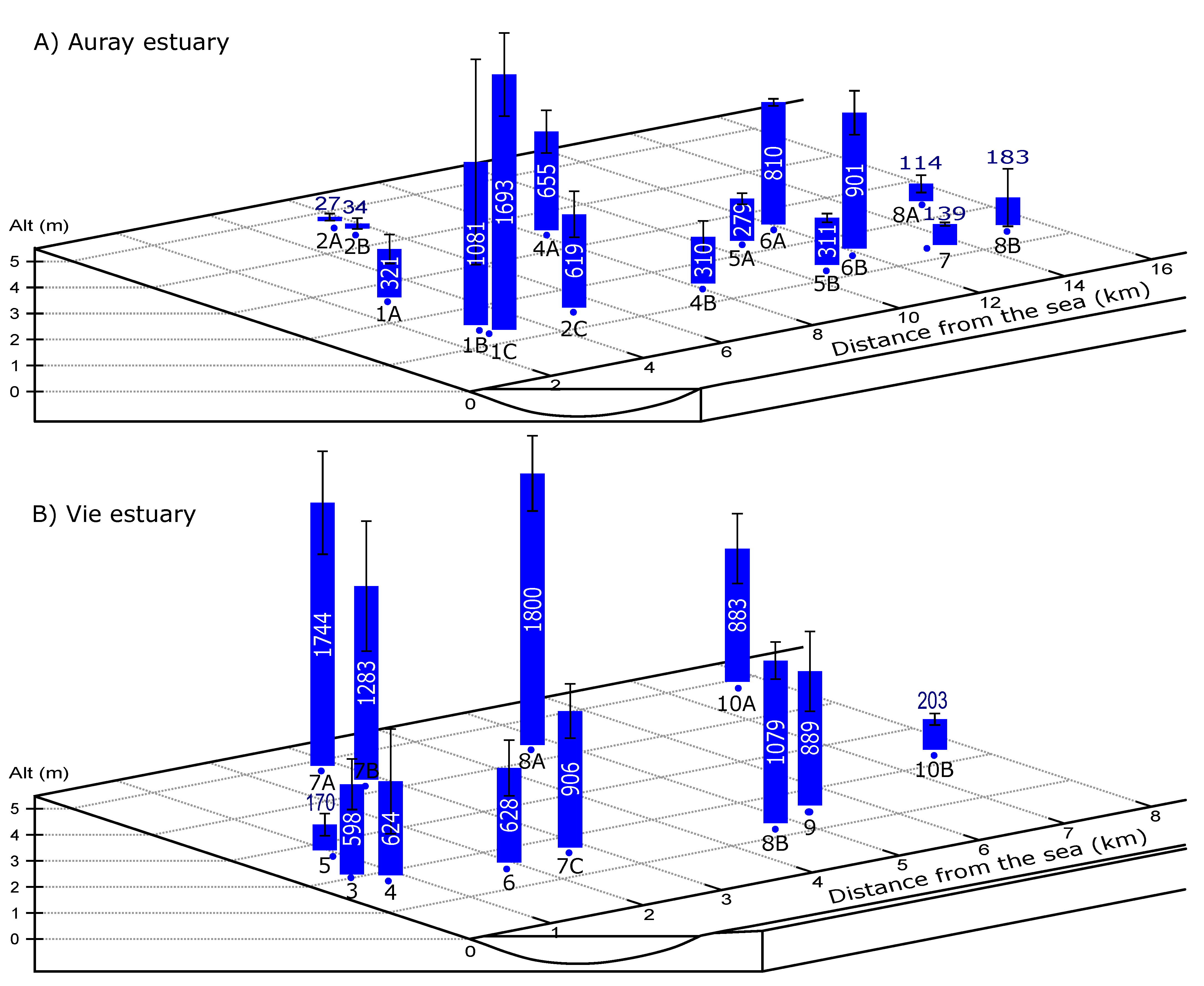
2.1. Study Area

In this study, the foraminiferal communities from intertidal mudflats of two small estuaries (~20 km long) on the French Atlantic coast, Auray and Vie, are investigated. Both estuaries are subject to a meso- to a low macrotidal regime, with a tidal range of about 4 m at the inlet [41].

The Auray estuary (Figure 1A and Supplementary Table S1), at about 47°35′ N and 2°57′ W, is a typical ria (drowned river valley) with its downstream part, or outer estuary, connected to the Morbihan Gulf, an enclosed marine bay. Two rivers flow out into the Auray estuary, the Loc’h and Bono, with a mean annual discharge of 2.71 and 1.52 m³/s, respectively [42]. Together, they drain a catchment area of 324 km². Today, salt water penetrates up to the Tréauray Mill, 19.8 km from the mouth of the estuary at Kerpenhir Point [41]. During the 2019 environmental survey in the context of the Marine Framework Directive, based on data collected between 2012 and 2017, the environmental quality was described as “moderate” [43]. This evaluation was exclusively based on an indicator using fishes. Conversely, indicators based on opportunistic macro-algae, autotrophs other than phytoplankton, and hydromorphology all indicated a good environmental quality.

The Vie estuary (Figure 1B and Supplementary Table S1), situated at about 46°35′ N and 1°56′ W, can be characterised as a bar-built estuary. The river meanders through salt marshes before crossing the Saint-Gilles-Croix-de-Vie harbour to flow into the Atlantic Ocean. Its mouth is deflected northwards by a sandy spit. The Vie river drains a catchment basin of 84 km² and has a mean annual discharge of 1.17 m³/s [41,42]. At present, salt water penetrates up to 8 km landward where it is blocked by a dam. Based on the thalweg topography, Jorissen et al. [40] deduced that before the construction of this dam, salt water penetrated up to the village of St. Maixent, 16.8 km from the mouth of the estuary. A 2019 environmental survey, performed in the context of the Marine Framework Directive, evaluated the environmental quality as “good”, on the basis of intertidal and opportunistic macroalgae and autotrophs other than phytoplankton [43].

2.2. Sampling Procedure

In the Auray estuary, seven sites (Site 3 is not considered in this study), with a total of 15 stations, were sampled from the 10th to 12th of July 2019 (Figure 1A). Samples of the surficial sediment (top centimetre) were collected at low tide on intertidal mudflats. At each site, two or three stations were sampled across the mudflat if it was large enough (A to C from upper mudflat to lower mudflat, Supplementary Table S2). In the Vie estuary, eight sites (Sites 1 and 2, located on sandy beaches outside the estuary, are not considered in this study), with a total of 12 stations, were sampled on the 23rd and 24th October 2018 (Figure 1B). Most stations are located on intertidal mudflats, except for stations 4 and 5, which are positioned on mud-covered ramps in small semi-enclosed basins in the harbour of Saint-Gilles (Supplementary Table S2).

To study the distribution of foraminifera, three replicates were sampled for each station. Three tubes with an internal diameter of 9.6 cm were randomly placed and pushed by hand into the sediment. The top 1 cm of the sediment cores was sliced off. Samples for foraminiferal analyses were preserved in 96% ethanol and stained with 2 g/L Rose Bengal, following the FOBIMO protocol [44]. Samples for grain size and organic matter analyses were taken between the cores by scraping off the surficial sediment layer.

For all sampling stations, the elevation was estimated with respect to French chart datum (lowest astronomical tide). For the stations sampled at low tide immediately above the water table, elevation was estimated using the tide tables published by the French Naval Hydrographic and Oceanographic Service (SHOM) [45], which give the theoretical altitude of the water surface during the tidal cycles for all French harbours. For all stations higher on the mudflats, the altitude was estimated using an electronic theodolite (NA720^® Leica; height accuracy <1 cm), and official benchmark altitude points. At stations located too far from referenced benchmarks, the lichen vertical zonation [46], developed on rocky outcrops and walls (quay, jetty, wharf…), was used. The conspicuous upper limit of the black lichen Verrucaria maura corresponds to the mean highest spring tide level, for which the altitude is given in the tide tables of the SHOM. Furthermore, this limit is highlighted by the lower limit of the orange lichen Xanthoria parietina, which marks the beginning of the supratidal zone. Taking into account the field constraints (and the uncertainty in the lichen vertical zonation) a range of uncertainty of +/−10 cm was estimated for our elevation data. By combining elevation and tide tables from the SHOM (based on the TELEMAC-MASCARET modelling system), it was possible to evaluate for each station the duration of the tidal emergence. The theoretical emergence time was estimated using tidal data corresponding to mean spring tide conditions (i.e., the French tidal coefficient of 90). The “emergence time” was then expressed as a percentage of the duration of an entire mean spring tide cycle.

Salinity was measured in the tidal channel for the lowest stations, and in tidal pools for the stations higher on the mudflats. In view of the large temporal variability in salinity [47,48], not only on the exposed mudflats (due to evaporation and precipitation) but also in the tidal channel (due to tide and river runoff), such one-off measurements are not representative for the foraminiferal habitat. Consequently, they are not further used in this study.

2.3. Laboratory Analyses

Sediment grain size was analysed with a Malvern 3000 Mastersizer laser diffraction particle size analyser. The sediment was not decarbonated before the analyses. To give an overall characterisation of the sediment, the percentage of grains < 63 µm was used. The grain size distribution spectra were further analysed with the Peakfit^® software (version 4.12), which allows for distinguishing and quantifying different sediment grain size populations. The classification proposed by Farrell et al. [49] was used for the description of the sediment.

Trace metal concentrations were analysed with an Inductively Coupled Plasma Mass Spectrometer (Thermo Scientific^® X-Series 2 ICP-MS) on freeze-dried sediment, after total acid digestion (HCl, HNO₃⁻ and HF) following the methodology described by Coynel et al. [50]. In all, seventeen chemical elements were measured: V, Cr, Co, Ni, Cu, Zn, As, Sr, Mo, Ag, Cd, Sn, Sb, Ba, Pb, Th and U. All concentrations are expressed in mg/kg. The natural variability in trace metal concentrations depends on the grain size and mineralogical composition. To correct for grain size and mineralogical effects, trace metal concentrations need to be normalised by a reference (conservative) element. Following earlier studies [51,52], Thorium (Th) was used for this purpose. The Enrichment Factor (EF) quantifies anthropogenic metal enrichment in the sediment. The EF is obtained by dividing the Th-normalised concentration by the concentration found in an unpolluted reference sediment, representative of the regional geochemical background [53]. Several studies have demonstrated that the regional geochemical backgrounds can be defined via the bottom/base of sediment cores in French continental systems, especially when the age model suggests that those deeper layers have been deposited before the onset of regional contamination sources (e.g., [54,55,56,57]). To this end, values from the basis of a long sediment core sampled in the western part of the Morbihan Gulf [58] have been used. These samples date from about 5000 years ago (5182 cal BP), well before the major anthropogenic activities of today.

The enrichment factor is calculated as follows:

$$EF=\frac{\frac{M}{Th}obs}{\frac{M}{Th}ref}$$

where M is the trace metal concentration, Th is the concentration of the conservative element, obs is the measured value and ref is the value of the geochemical background as observed in the sediment core samples. Following Larrose et al. [52], enrichment classes are defined as follows:

• EF < 1.5: no enrichment;
• 1.5 < EF < 3: minor enrichment;
• 3 < EF < 5: moderate enrichment;
• EF > 5: strong enrichment.

Elemental carbon content (%C_org) and the carbon isotopic composition (δ¹³C) were measured on decarbonated freeze-dried sediment with a CHONS Elemental Analyser (EA Vario PYRO cube; Elementar^®, Langenselbold, Germany) coupled to an isotope ratio mass spectrometer (IRMS; Isoprime precision, Elementar^®, Langenselbold, Germany). Prior to EA-IRMS analysis, 300 mg of dried sediment was decarbonated with phosphoric acid to remove inorganic carbon (H₃PO₄, concentration 2 M). After decarbonatation, samples were freeze-dried and ground. Three milligrams of samples were weighed in tin capsules. Possible offsets of raw IRMS values were corrected using both international IEAE (Vienna) and home-made standards (caffeine IAEA-600- and a sucrose-methionine-glycine mixture, referred to as SMG and cross-calibrated against caffeine IAEA-600 and Ag₂S IAEA-S-1, for C, N and S isotopes). Note that the linearity of the IRMS response was checked throughout to be less than 0.02‰ nA⁻¹, and furthermore, any possible size effect between samples was minimised by weighing the same amount for all samples. Standards (which had a %C_org different from that of samples) were weighed accordingly to have the same signal intensity. All isotopic data are expressed in the conventional delta notation versus V-PDB (‰): δ¹³C_sample = (R_sample/R_V-PDB − 1) × 1000 with R = ¹³C/¹²C [59].

Foraminiferal samples were sieved with 63, 125 and 500 µm meshes, and the fraction >125 µm was used for foraminiferal analyses. Although the >125 µm fraction contains only a part of the foraminiferal community, the study of this fraction has the advantage of being less time-consuming than that of the >63 µm or 100 µm fraction. Therefore, the experimental design can include more samples. Moreover, since >125 µm sufficiently reflects the foraminiferal community, the FOBIMO protocol proposes the study of this size fraction as an optimal compromise for biomonitoring studies [44]. When necessary, density separation using Ludox to remove organic material [60,61] or sodium polytungstate to remove sand [62] was applied. Samples with a high foraminiferal density were divided in aliquots using a wet splitter [63]. Foraminifera were picked wet, using a Leica MZ16 stereomicroscope, and stored in Chapman slides. All stained individuals (all chambers except the last one or two brightly stained pink) were considered living. Complete aliquots were counted until a minimum of 300 specimens was obtained [64,65].

All hard-shelled foraminifera were identified to the species level (Figure 2), using classical and modern reference publications on estuarine foraminifera (i.e., [66,67,68,69,70]), as well as the World Register of Marine Species [12]. Studies combining genetic and morphological information were favoured to identify the Ammonia and elphidiid species [71,72,73]. The previously recognised morphospecies Ammonia tepida is composed of three different phylotypes in Europe (T1, T2 and T6, [74]), which can be distinguished morphologically [75]. Following earlier studies (e.g., [75]), we will refer to the Ammonia tepida group when speaking about this morphospecies, which includes phylogenetically unrelated phylotypes. With a stereomicroscope, it was mostly impossible to differentiate between these three phylotypes, particularly for small specimens. Consequently, in order to determine the presence/absence of the phylotypes’ diversity in the Ammonia tepida group, 50 randomly sampled individuals per station were identified on the basis of SEM images, following Richirt et al. [75].

2.4. Marine Influence Index

The Marine Influence Index proposed by Jorissen et al. [40] was tested in this study. The MII combines the position of the sampling site along the estuarine gradient, the duration of the tidal emergence, as well as the riverine fresh water input during the 30 days before sampling. The MII has been designed to give an integrated quantitative estimation of the influence of marine waters at the sampling stations. This index was calculated as follows:

$$\mathrm{MII}=\left(1-\frac{\mathrm{x}}{\mathrm{s}}\times \mathsf{\alpha }\right)\times \left(1-\mathrm{ET}\times \mathsf{\beta }\right)\times \left(1-\sqrt{\frac{0.04\times \mathrm{RD}}{\mathrm{CS}}}\times \mathrm{y}\right)$$

The first term of the equation is the normalised distance, in which x is the distance of the sampling site from the mouth of the estuary measured along the main estuarine channel, divided by s, the length of the salt intrusion. The second term refers to the normalised emergence time, in which ET, the duration of the tidal emergence at a sampling station, is expressed as a fraction of the tidal period, under mean spring tide conditions. The third term considers the relative river discharge, in which RD (m/s) is the diver discharge in the 30 days before sampling, and CS is the cross section (m²) of the estuary at the study site, measured at mean high tide. α, β and γ are constants, used to weigh the three components of the equation. In this study, these constants are set to 1, giving equal weight to the three components. See Jorissen et al. [40] for further explanations. The values of MII computed for this study are presented in Supplementary Table S10.

2.5. Statistical Analyses

All diversity indices (species richness, Shanon index, exp(H’bc index)) were based on raw data, using R software (version 4.0.4) [76] and the “vegan” package (version 2.5–7, [77]). The calculation of the Foram-AMBI index was based on the species assignment list proposed by Bouchet et al. [25].

A non-standardised Principal Components Analysis (PCA) was performed on non-transformed percentage data using the variance–covariance matrix. PCA reduces data matrices to a small number of factors explaining a maximum of the total variance. Only species exceeding 1% of the assemblage in at least one station were taken into consideration. Relevant variables were selected by forward selection based on PCA (ordistep function, R package “vegan”). Next, the environmental parameters were fitted to the PCA axes using the envfit function of the R package “vegan” (non-constrained version, the environmental parameters did not contribute to the ordination). All environmental data were standardised.

For all correlation tests, the normality of the data set was tested using the Shapiro–Wilk normality test, and the homogeneity of variance (homoscedasticity) with the Bartlett test. Finally, Pearson or Spearman correlation tests were applied. A trend line was fitted to each scatter plot. For regression lines, the generalised linear model (“glm”) was used except when a nonlinear regression (“nls”) was found.

3. Results

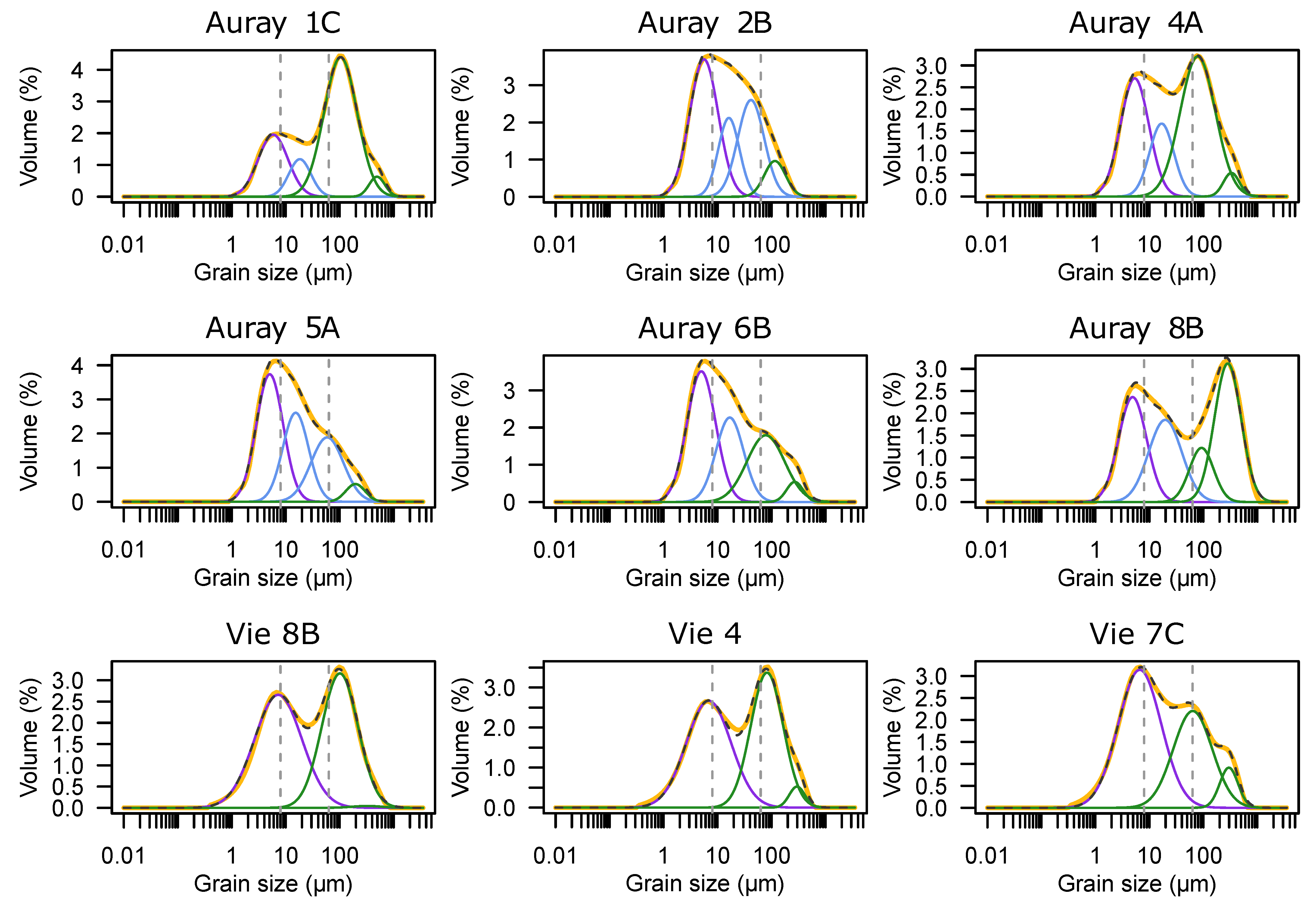
3.1. Sediment Grain Size

All seven sites in the Auray estuary presented a silty–muddy sediment with ≥50% fine (<63 µm) grains (Figure 3, Supplementary Table S3). A particle population with a mode of about 5 µm was dominant at almost all stations (e.g., Auray 2B, 5A, 6B shown on Figure 3), while this 5µm mode became secondary at stations 1B, 1C, 4A and 8B. A silt/very fine sand population, with a mode of 30 to 105 µm, was dominant at all stations of sites 1 and 4. At sites where more than one station was sampled, the mode of the latter population increased towards the lower elevation. Station 8B was the only one with an important medium sand population, with a mode of 284 µm.

In the Vie estuary, all sites had a silty–muddy sediment, with two dominant populations, a first one with a mode of 6 to 10 µm, and a second one with a mode of 40 to 100 µm (Figure 3, Supplementary Table S3). For both estuaries taken together, there is a positive correlation between elevation and the percentage of fine (<63 µm) grains (R² = 0.14, p = 0.056).

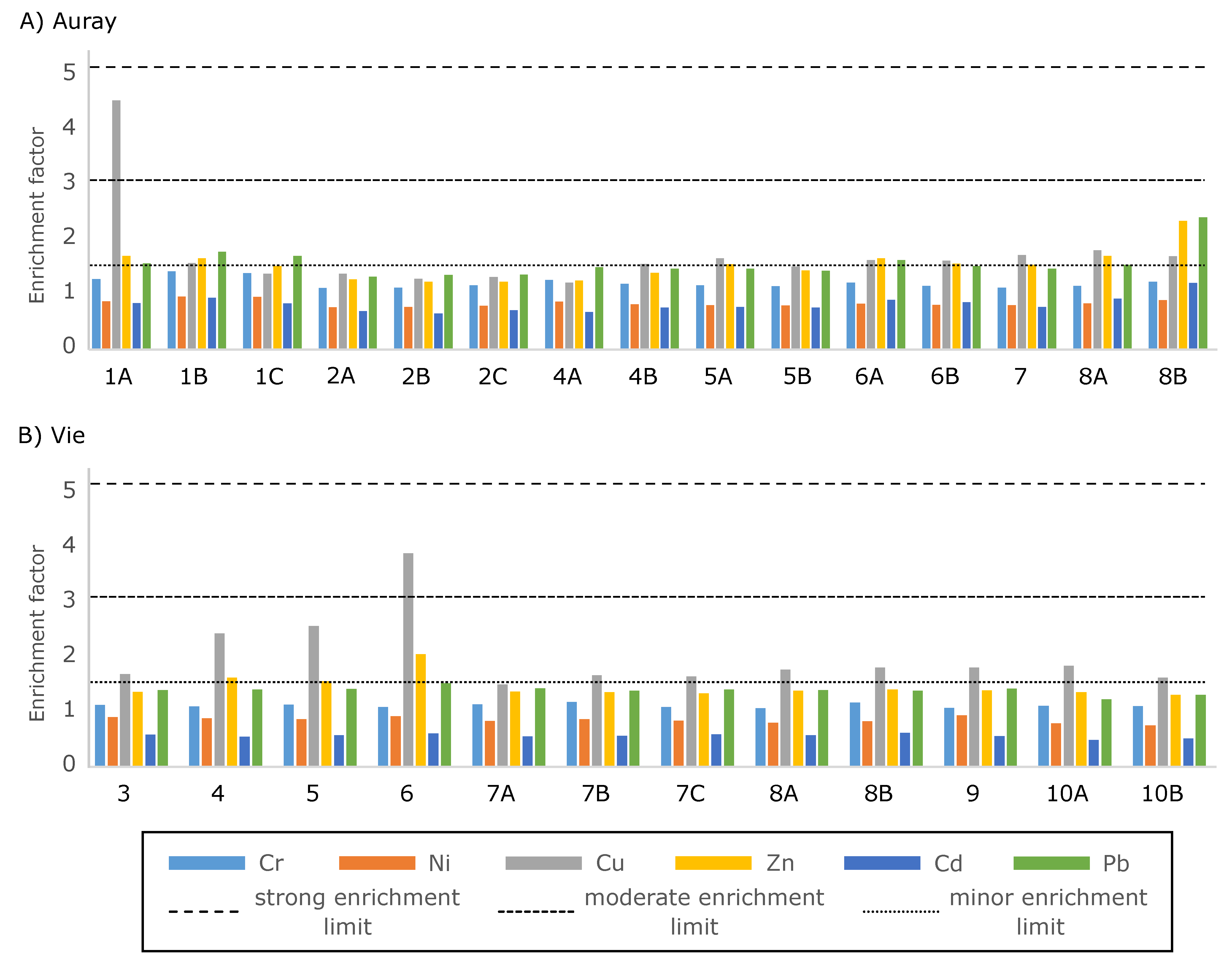
3.2. Trace Metal Distribution

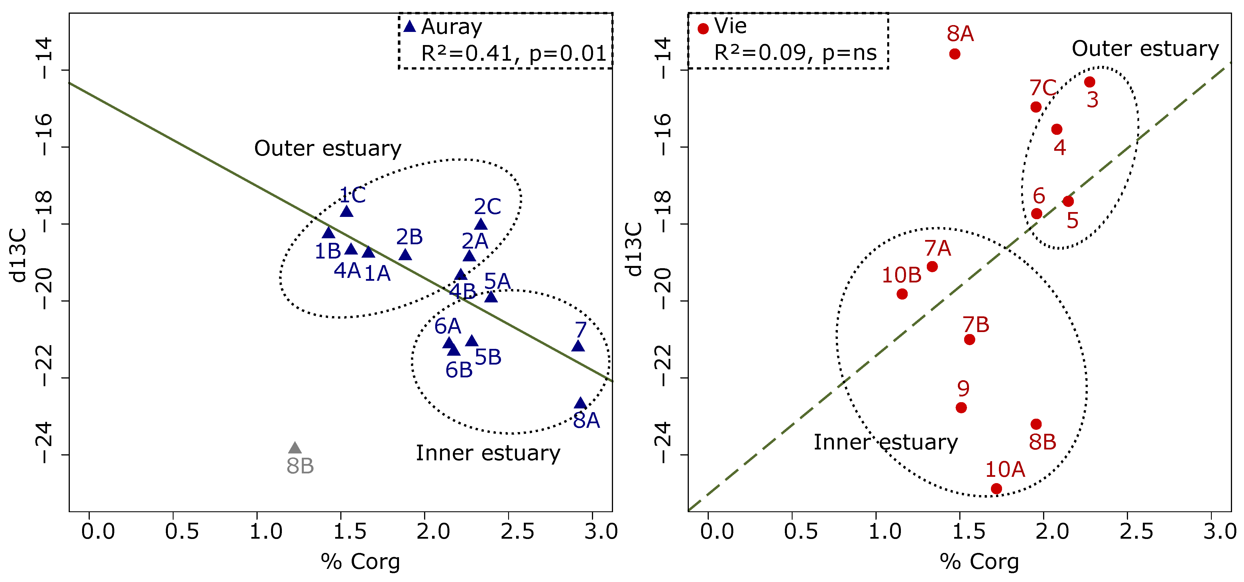
At the 27 stations, 17 trace metal elements were measured (Supplementary Table S4). The raw values for all trace metals were slightly higher in the Auray estuary compared to the Vie estuary, which is probably the result of a different geology of the catchment area (Supplementary Table S4). Enrichment factors (EFs) were computed for the six main trace elements (Cr, Ni, Cu, Zn, Cd, Pb) that could have an impact on community composition. In the Auray estuary, the EFs of trace metals were in the same range at all stations, except for Cu at station 1A (increased by a factor three), and station 8B, where Zn and Pb showed slightly raised values. Additionally, in the Vie estuary, the EFs were similar at all stations, except for Cu at stations 4, 5 and especially 6, where the EFs were 1.5 to 2.5 times higher than everywhere else (Figure 4).

3.3. Organic Matter

The percentages of C_org and δ¹³C measurements are presented in Supplementary Table S5. In the Auray estuary, the percentage of acid-resistant carbon in sediment samples (%C_org) varied from 1.23 to 2.93% (Figure 5; Supplementary Table S5). In general, %C_org was higher in the inner (2.15–2.93%) than in the outer estuary (1.43 to 2.33%), except for station 8B, with a low value of 1.23%. There was no systematic trend between higher and lower stations on mudflats. The δ¹³C (Figure 5; Supplementary Table S5) varied from –17.71 to –23.86‰, with a gradient from high values in the outer estuary (sites 1,2 and 4) to lower values in the inner estuary (sites 5, 6, 7 and 8).

In the Vie estuary, the %C_org varied from 1.16 to 2.27% (Figure 5; Supplementary Table S5). Values were higher in outer estuary (1.96 to 2.27%) than in the inner estuary (1.16 to 1.96%). Similar to in the Auray estuary, there was a trend of decreasing δ¹³C (Figure 5; Supplementary Table S5), from –14.3‰ in the outer estuary (station 3) to –24.9‰ in the inner estuary (station 10A). However, this tendency was weakened at two stations (7C and 8A) with a high δ¹³C compared to the other inner estuary stations.

The comparison of the %C_org with the δ¹³C shows different patterns for the two estuaries (Figure 5). In the Auray estuary, these parameters show a significant negative correlation (R² = 0.41, p-value = 0.01) when station 8B, with a very different sediment grain size (medium sand), is not included in the analysis. In the Vie estuary, the correlation is not significant.

3.4. Foraminiferal Distribution

3.4.1. Density

In the Auray estuary, the average foraminiferal density in the >125 µm fraction (based on the study of three replicates at each station) varied from ~25 to ~1700 individuals per 50 cm³ (Figure 6; Supplementary Table S6), without a clear spatial trend. Although the three replicates had comparable values for many stations, at stations 1B, 2A, 2B and 8B, the richest replicate was up to 10 times richer than the poorest one, suggesting considerable spatial patchiness at a decimetric scale. At several stations, foraminifera with a dissolved shell as well as organic linings were observed, but were not counted.

In the Vie estuary, the average foraminiferal density (for 3 replicates) varied from ~170 to ~1800 foraminifera per 50 cm³ (Supplementary Table S7), again without a clear spatial tendency (Figure 6). The three replicates had comparable values. At all sites with a large mudflat (sampled on a cross-shore transect), the densities increased towards higher elevation.

3.4.2. Foraminiferal Diversity

The total dataset contains 41 species (in the >125 µm fraction), of which 14 are common to both estuaries.

In the Auray estuary, 27 species were identified. Species richness (

Table 1. Diversity indices in the Auray estuary. For every station the average of the three replicate samples is given.

Estuary	Station	Species Richness	Shannon	Exp(H’BC)
Auray	1A	8.0 (±2.0)	0.68 (±0.16)	2.01 (±0.31)
	1B	10.7 (±1.2)	1.44 (±0.08)	4.22 (±0.30)
	1C	12.7 (±2.5)	1.65 (±0.13)	5.23 (±0.72)
	2A	2.0 (±1.7)	0.15 (±0.28)	1.37 (±0.63)
	2B	4.3 (±4.9)	0.40 (±0.53)	1.80 (±1.02)
	2C	8.0 (±1.0)	0.80 (±0.16)	2.26 (±0.33)
	4A	8.7 (±1.5)	0.64 (±0.26)	1.95 (±0.48)
	4B	8.0 (±1.0)	0.62 (±0.17)	1.92 (±0.31)
	5A	5.0 (±1.7)	0.12 (±0.03)	1.14 (±0.05)
	5B	11.7 (±2.3)	0.86 (±0.24)	2.49 (±0.57)
	6A	7.3 (±0.6)	0.30 (±0.17)	1.37 (±0.24)
	6B	11.7 (±0.6)	0.73 (±0.26)	2.14 (±0.54)
	7	5.7 (±1.2)	0.69 (±0.04)	2.02 (±0.09)
	8A	8.3 (±1.2)	1.27 (±0.14)	3.73 (±0.34)
	8B	5.3 (±2.3)	0.68 (±0.29)	2.07 (±0.56)
Vie	3	14.3 (±1.5)	1.14 (±0.20)	3.17 (±0.27)
	4	12.3 (±2.5)	1.09 (±0.35)	3.10 (±1.07)
	5	9.3 (±2.3)	0.87 (±0.04)	2.45 (±0.30)
	6	9.0 (±2.6)	0.68 (±0.17)	2.00 (±0.31)
	7A	8.3 (±1.2)	0.33 (±0.01)	1.40 (±0.01)
	7B	8.0 (±0.0)	0.40 (±0.11)	1.50 (±0.15)
	7C	10.7 (±0.6)	0.99 (±0.16)	2.72 (±0.41)
	8A	9.7 (±0.6)	1.19 (±0.07)	3.30 (±0.19)
	8B	7.3 (±0.6)	0.65 (±0.11)	1.92 (±0.20)
	9	9.7 (±0.6)	1.20 (±0.12)	3.33 (±0.06)
	10A	8.7 (±0.6)	1.03 (±0.10)	2.84 (±0.34)
	10B	7.3 (±0.6)	0.71 (±0.22)	2.05 (±0.15)

) varied between 4 and 13, the Shannon index from 0.12 to 1.65 and Exp(H’_BC) from 1.14 to 5.23, without a clear tendency. However, at most sites with large mudflats (more than one station), there was a gradient from high values in the lower parts (stations B and C, lower elevation) to low values in upper parts (station A, higher elevation) of the mudflat.

In the Vie estuary, 28 species were recognised. Here, species richness varied between 7.3 and 14.3, the Shannon index from 0.18 to 0.63 and Exp(H’_BC) from 1.40 to 3.33 (Table 1). Most indices had raised values at sites 3 and 4, in the outer estuary. At site 7, where three stations were sampled at different altitudes, all diversity indices increased from the highest (7A) to the lowest station (7C). However, this tendency was not observed at sites 8 and 10, where two stations were sampled.

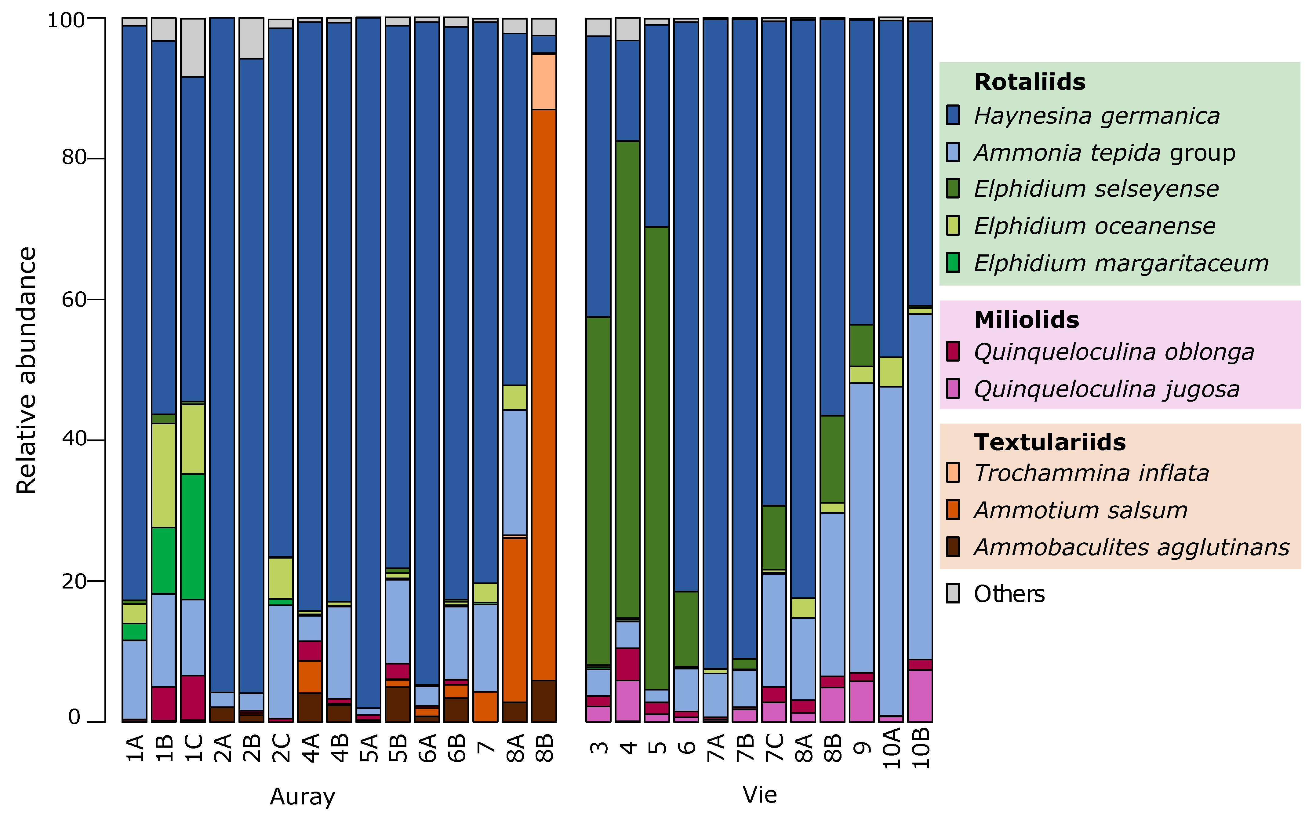
3.4.3. Foraminiferal Communities

In the Auray estuary, 16 species were found at least at one station with an average relative frequency higher than 1% for the three replicates (Plate 1, Supplementary Table S8). Eight of these species were rotaliids (calcareous perforate test), seven were textulariids (agglutinated test) and one was a miliolid (porcelaneous test). Rotaliids accounted for more than 88% of the foraminifera, except at stations 8A and 8B, in the inner estuary, where textulariids were abundant (Figure 7). Miliolids were present at all stations but represented at most 6.5% of the relative abundance. At all stations except 8B, Haynesina germanica was dominant (50–96%). The Ammonia tepida group was present in the whole estuary (except at 8B), with values up to 18%. It showed much lower percentages at all stations at higher elevation (2A, 2B, 4A, 5A, 6A). Phylotype Ammonia sp. T1 was dominant (about ~75%), and was accompanied by Ammonia sp. T2 (~20%) and sp. T6 (~5%), without a clear spatial tendency. Elphidiids were mostly present in the outer estuary (site 1), at stations of lower elevation (1B, 1C, 2C), where they reached up to 30%, and were mainly represented by Elphidium margaritaceum and Elphidium oceanense. Elphidium margaritaceum was only observed at sites 1 and 2, while E. oceanense was also present in the inner estuary, but with lower densities. The agglutinated species, especially frequent at stations 8B (95%) and 8A (27%), were dominated by Ammotium salsum, with a minor contribution of Trochammina inflata and Ammobaculites agglutinans. Among the miliolids, Quinqueloculina oblonga occurred at almost all stations, with a maximum at 1B and 1C, whereas Quinqueloculina jugosa was rare, and never attained 1%.

In the Vie estuary, eight species were found at least at one station with an average relative frequency larger than 1% for the three replicates (Plate 1, Supplementary Table S9). Six of these species were rotaliids, whereas the other two were miliolids. Rotaliids always accounted for most of the foraminiferal community (89–99%). Miliolids (Q. jugosa and Q. oblonga) were present at all stations, with a maximum of 10.5%. The sampling sites can be divided into three zones (Figure 7). At sites 3, 4, and 5, the assemblages were dominated by Elphidium selseyense (49–78%). The three sites in the middle estuary (6, 7 and 8) were dominated by H. germanica (56–92%), whereas E. selseyense dropped to low values (12.4% or less). Elphidium selseyense was virtually absent at the stations of highest elevation (7A, 8A and 10A). Towards the inner part of the estuary, the Ammonia tepida group increased, to become dominant (41–49%) at stations 9, 10A and 10B. At stations were the Ammonia tepida group was abundant, phylotypes T1 (~50%) and T6 (~40%) were dominant (~75%), accompanied by T2 (10%), without a clear spatial pattern. Miliolids (essentially Q. jugosa and Q. oblonga) showed slightly raised percentages at stations 4, 8B, 9 and 10B.

For all dominant species, correlations with the main environmental parameters and with MII were calculated (Supplementary Table S12). Elphidium selseyense and Q. oblonga are both negatively correlated with emergence time, whereas H. germanica shows a positive correlation with this factor in the Auray estuary. Ammobaculites agglutinans and Ammotium salsum show a negative correlation with the distance to the sea, as does the A. tepida morphogroup and E. oceanense in the Vie estuary. Elphidium selseyense is the only taxon showing a negative correlation with the sediment fine fraction. Finally, E. selseyense and H. germanica are positively correlated with %C_org, whereas Q. oblonga shows a negative correlation.

The non-standardised PCA model based on percentage data of the dominant species yields three significant axes that explain, respectively, 58.2, 23.3 and 15.4% of the total variance (Figure 8). The eigenvalues and species loadings on the three axes are listed in Supplementary Table S11.

The three first PCA axes are dominated by the four most common taxa. Haynesina germanica has a high positive loading on axis 1, whereas E. selseyense and A. salsum have a negative loading. The second PCA axis is positively loaded by E. selseyense and H. germanica, and negatively by A. salsum and the A. tepida group. Finally, the third axis is driven by the A. tepida group and A. salsum.

The ordination model is determined by a small number of stations with very distinct foraminiferal communities (Figure 8). This concerns especially station 8B of Auray and stations 3, 4 and 5 of the Vie estuary. Station 8B of Auray is in the negative domain of both axis 1 and axis 2, because of the high percentage of A. salsum. The position of stations 3, 4 and 5 of the Vie estuary (negative on axis 1, positive on axis 2) is explained by their high percentage of E. selseyense.

For the remaining samples, the axial plot of PCA1 and PCA2 shows an overlap between the two estuaries, with samples being organised mainly along PCA1, largely as a function of the percentage of H. germanica. For most sites where several stations were sampled at different altitudes, the higher samples (with longer emergence times) have higher values on PCA1.

The axial plots of PCA1 and PCA3 show that PCA3 mainly distinguishes the inner estuary stations 9, 10A and 10B of the Vie estuary, which have high scores on PCA3, due to a high proportion of the A. tepida group.

Both the normalised distance to the sea (R² = 0.46, p = 0.001) and the <63 µm grain size fraction (R² = 0.30, p = 0.05) show significant correlations with the PCA model. No significant correlations were found for the %C_org and the normalised emergence time (

Table 2. Envfit results: multiple regression of environmental variable with ordination axes.

	PCA1	PCA2	PCA3	R2	p-Value
% Corg	0.37	0.78	−0.51	0.15	0.29
<63 µm grain size	0.88	0.26	0.40	0.30	0.05 *
Distance to the sea	−0.13	0.98	0.12	0.46	0.001 *
Emergence time	−0.96	−0.15	0.24	0.16	0.24

Note: * indicate significant p-values.

).

3.4.4. Foraminiferal Indices of Environmental Quality

In the Auray estuary, at all stations except station 8B (Foram-AMBI: 1.41), the values of Foram-AMBI varied between 2.57 and 3.02, resulting in a good quality status (1.2 < Foram-AMBI < 3.3), although close to the upper limit of this category (

Table 3. Results of the Foram-AMBI on Auray and Vie stations and associated ecological quality status (<1.2: High; 1.2-3.3: Good; 3.3-4.3: Moderate; 4.3-5.5: Poor; >5.5: Bad).

Auray	Station	Foram-AMBI	Ecological Quality Status	Vie	Station	Foram-AMBI	Ecological Quality Status
	1A	2.92 ± 0.01	Good		3	1.49 ± 0.14	Good
	1B	2.83 ± 0.05	Good		4	0.95 ± 0.51	High
	1C	2.56 ± 0.10	Good		5	1.04 ± 0.04	High
	2A	2.97 ± 0.05	Good		6	2.68 ± 0.12	Good
	2B	2.90 ± 0.09	Good		7A	3.00 ± 0.01	Good
	2C	3.01 ± 0.06	Good		7B	2.94 ± 0.03	Good
	4A	2.95 ± 0.20	Good		7C	2.75 ± 0.16	Good
	4B	2.98 ± 0.00	Good		8A	2.60 ± 0.04	Good
	5A	3.02 ± 0.02	Good		8B	3.03 ± 0.03	Good
	5B	2.95 ± 0.06	Good		9	2.77 ± 0.08	Good
	6A	3.00 ± 0.03	Good		10A	2.93 ± 0.05	Good
	6B	2.94 ± 0.02	Good		10B	2.99 ± 0.00	Good
	7	2.93 ± 0.06	Good
	8A	2.57 ± 0.16	Good
	8B	1.41 ± 0.07	Good

). In the Vie estuary, stations 3 to 5 had values between 0.95 and 1.5 (high to good ecological quality), whereas for all other sites, the values varied from 2.60 to 3.03 (good ecological quality).

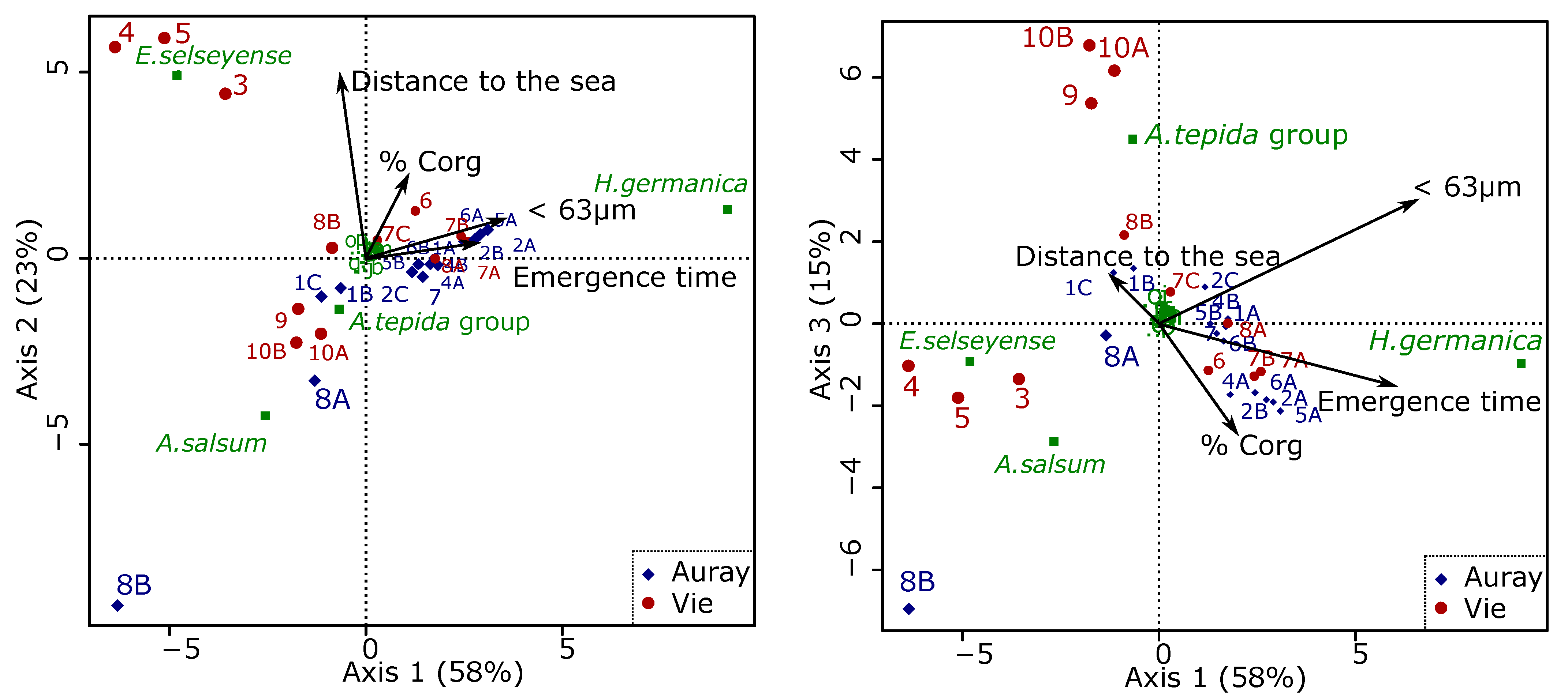
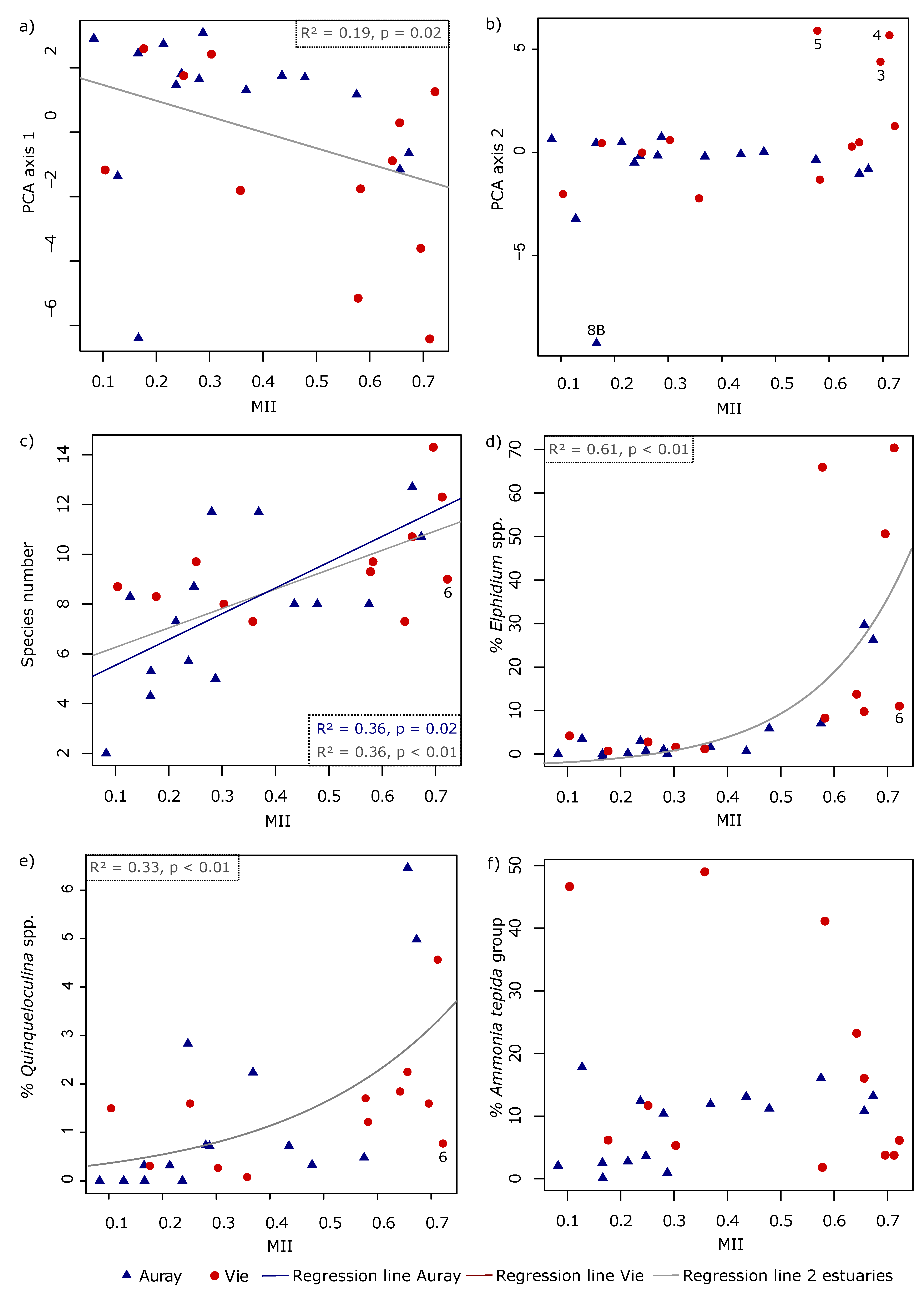
3.4.5. Relations between Foraminiferal Distribution and the Marine Influence Index (MII)

Jorissen et al. [40] suggested that the Marine Influence Index (MII) should explain part of the foraminiferal distribution in estuaries. MII values are presented in Supplementary Table S10. MII values are higher (more marine influence) in stations located near the mouth than those located in the inner part of the estuary. MII values are also higher on the lower part of the mudflat compared to the upper part. In Figure 9, the MII is compared with some major foraminiferal community characteristics. In Figure 9a,b, the MII is compared with the sample scores on PCA axes 1 and 2. A weak but significant correlation is found for PCA1 (R² = 0.19, p < 0.05). The separation of the four stations on PCA2 (negative side: Auray 8B; positive side: Vie 3, 4 and 5) is reflected by their contrasting MIIs, but because most stations hardly load on PCA2, the overall correlation is not significant. In Figure 9c, the MII is compared to species richness. A significant positive correlation is observed (R² = 0.36, p < 0.01) for the total dataset. The correlation is also significant for the Auray estuary alone (R² = 0.36, p < 0.05), but is not significant for the Vie estuary. Figure 9d shows the relationship between the MII and the percentage of Elphidium spp. There is a similar tendency for both estuaries, with less than 5% Elphidium spp. at all stations where the MII is lower than 0.45. Elphidiids only become a dominant foraminiferal component when the MII is higher than 0.5. The transition between these two domains is abrupt. Figure 9e shows a significant linear correlation (R² = 0.42, p < 0.01) between the MII and the percentage of Quinqueloculina spp. Finally, in Figure 9f, the relationship between the MII and the percentage of the Ammonia tepida group is shown. The absence of a significant correlation is partly explained by the distribution in the Vie, where high percentages (>40%) of this taxon are observed at three stations in the innermost part of the estuary (9, 10A, 10B) with different MIIs, mainly due to differences in emergence time. Correlations between all dominant species and MII are presented in Supplementary Table S12. Quinqueloculina oblonga (both estuaries), Elphidium margaritaceum (Auray), E. oceanense (Auray) and E. selseyense (Vie) are positively correlated with the MII, whereas Haynesina germanica shows a weak negative correlation with the MII.

4. Discussion

This paper focusses on the foraminiferal assemblages of intertidal mudflats of the Auray and Vie estuaries. Both estuaries are short coastal waterways of the French Atlantic coast, with relatively low riverine water supply, and a mesotidal to low macrotidal regime, but they present contrasting geomorphological characteristics. The Auray estuary is a ria, with a relatively deep channel connecting the outer estuary to the marine Morbihan Gulf, and as such is a marine-influenced estuary. Conversely, the Vie estuary is a lowland meandering waterway, potentially with a stronger riverine influence (Figure 1).

4.1. Environmental Characteristics

Besides the positions along the estuary and the altitudes of the individual sampling stations, three other environmental parameters were used to describe the foraminiferal habitat;

(I).

Sediment grain size—two dominant grain size populations coexist, which may correspond to a mix of sand deposits during high river discharge periods and the settling of clay-silt from riverine input during slack waters. There is a significant decrease in grain size towards stations higher on the mudflats where tidal currents are weaker;

(II).

Organic matter quantity and quality—different %C_org patterns underline the difference between the two estuaries. In the Auray estuary, the %C_org decreases seawards, whereas the opposite is observed in the Vie estuary. In fact, in the outer Auray estuary (sites 1 and 2), open to the sea, organically poor marine waters replace organically rich riverine waters. In both estuaries, δ¹³C shows an overall seaward decrease, which corresponds to the natural gradual transition of continental to marine organic matter [78,79]. In the outer Auray estuary, δ¹³C values vary from −18 to −20‰, suggesting a major contribution of microphytobenthos [59]. In the Vie estuary, the low values observed at several stations (between −14 and −16‰) could be related to the presence of macro-algae [59,80], which were observed during the sampling campaign. In summarising, it appears that both the %C_org and the δ¹³C trends reflect natural patterns that seem not be biased by anthropogenic organic matter input;

(III).

Trace metal concentrations—in both estuaries, none of the six trace metals considered relevant for biota attains the strong enrichment limit (as defined by Larrose et al. [54]). Concerning Cu concentrations, the moderate enrichment at stations Auray 1A and Vie 6 and the minor enrichment at stations Vie 4 and 5 may be related to antifouling paint used in the nearby harbours. Only minor Pb and Zn enrichment was detected (mainly at station Auray 8B).

Low concentrations of trace metals and organic matter suggest that, except for stations Auray 1A and Vie 6 (close to harbours), the studied estuaries are not subjected to strong anthropogenic pollution. This confirms the overall evaluation of the 2019 survey [43] of average (fish-based indicator) to good ecological quality (opportunistic macro-algae, plants other than phytoplankton and hydromorphology) for the Auray estuary and good quality (intertidal and opportunistic macroalgae and plants other than phytoplankton) for the Vie estuary. Therefore, in both estuaries, the ecosystems should be mainly controlled by natural environmental parameters.

4.2. Foraminifera Communities

The foraminiferal faunas observed in the two estuaries show comparable density and diversity (Figure 6, Figure 7 and Figure 8, Table 1 and Table 3). In the Auray estuary, Haynesina germanica and the Ammonia tepida group are dominant at almost all stations. In the outer estuary, open marine neritic species (e.g., Elphidium margaritaceum, Elphidium oceanense; see Supplementary Table S13 for an overview of the ecological characteristics of the dominant taxa) are more frequent. In the Vie estuary, an up- to downstream succession of the three main assemblages is observed, all dominated by taxa typical of estuarine ecosystems. Elphidium selseyense is dominant in the outer estuary, H. germanica in the middle estuary, and finally the A. tepida group is dominant in the inner estuary. This succession is in accordance with the literature, where A. tepida and H. germanica are commonly observed as dominant species in estuaries [27,81,82] where some Elphidium species may also be frequent (E. williamsoni [27,81]; E. oceanense ([27]; E. margaritaceum [83]; E. selseyense [82,83]).

In view of the absence of strong pollution, the Auray and Vie estuaries can be considered as model ecosystems, representative of the environmental quality found today in most human-influenced, relatively weakly polluted estuaries. However, these two estuaries are obviously not pristine, but subjected to anthropogenic influences. The Vie estuary is closed upstream with a dam, whereas the outer estuary crosses an urbanised area (Saint-Gilles-Croix-de-Vie), with a marina and a fishing harbour (Figure 1B). The Auray estuary is under high touristic pressure and is also an important centre for oyster farming. Even if metal enrichment is only minor or moderate, we cannot exclude the possibility that the combined effects of raised trace element concentrations and other stressors can affect the foraminiferal communities. In order to recognise the eventual impacts of multiple stresses, we will investigate (1) whether the moderate enrichment in Cu at two stations has affected the foraminiferal communities there, and (2) whether some deviating foraminiferal assemblage characteristics can eventually reflect localised pollution.

At the upper mudflat station Auray 1A, next to the harbour of Locmariaquer, moderate Cu enrichment was observed. However, the foraminiferal community was similar to that found at nearby (not Cu-enriched) stations (1B, 1C, 2C; Figure 7). Similarly, at station Vie 6, a moderate Cu enrichment was also measured. The foraminiferal community at this station seemed to be intermediate between those found at the nearby sites 5 and 7 (Figure 7). Apparently, there is no foraminiferal community response to the moderate Cu enrichment observed at these stations.

Two groups of stations stand out by their particular faunal composition; they are strongly opposed on PCA axis 2 (Figure 8):

(1).

The foraminiferal assemblage at station Auray 8B is composed by more than 90% agglutinated species (Ammotium salsum, Ammobaculites agglutinans, Trochammina inflata). These agglutinated species, typical of oligohaline conditions, are commonly found in salt marshes [28,84,85] and may also occur in inner estuaries [86]. This assemblage is compatible with the low salinity recorded (about 16 at high spring tide). Station 8B also stands out because of its much higher proportion of medium sand. Very close to station 8B, the estuary artificially narrows to a single channel to pass under a road bridge, leading to a higher current velocity (Figure 3). This brackish and dynamic hydrological setting could explain the very different foraminiferal community observed at this station;

(2).

In the Vie estuary, stations 4 and 5 have been sampled on concrete shipping ramps, covered with several-decimetres-thick mud deposits, inside docks in the St-Gilles-Croix-de-Vie harbour, and undergo strong anthropogenic influence. This is partly evidenced by the slightly increased Cu concentrations at these two stations (Figure 4), corresponding to minor enrichment [51]. At these stations the foraminiferal community shows high abundances of E. selseyense. In view of the preference of E. selseyense for the outer estuary [86], and the occurrence of a similar community at station 3, where no increased Cu-content was observed, it seems unlikely that its dominance at these stations reflects strong pollution.

In conclusion, the foraminiferal patterns in both estuaries seem to be controlled by natural parameters. There is no indication that the different composition of the foraminiferal community at the sites discussed above is a response to anthropogenic pollution.

4.3. Comparison with Previous Studies

The foraminifera of the Auray and Vie estuaries have been extensively studied in the past [87,88,89]. Unfortunately, there are some important methodological differences between our study, using the recently proposed FOBIMO sampling protocol [44], and these former studies, especially with respect to the determination of living specimens (by Rose Bengal staining), the preservation procedure and the studied size fractions. Although a detailed comparison is not possible, some observations can be made on the basis of these studies.

The Auray estuary was studied in 1994 by Redois [87]. The areas corresponding to our sampling sites show the same main species: Haynesina germanica, Ammonia tepida, Quinqueloculina oblonga (determined as Q. seminula forma 2), Elphidium oceanense (determined as Cribroelphidum gunteri), E. margaritaceum (determined as E. pulvereum) and Ammonium salsum. At our site 8, the only one where A. salsum substantially contributes to the foraminiferal community (23% at 8B, 81% at 8A), Redois also observed this agglutinated species, at a maximum of 9%. In the middle estuary (stations 4 and 5), Redois [87] described Q. oblonga as a major species (up to 55%), while this is only a minor species (<6.3%) in our samples. This may be explained by the fact that Redois analysed the >50 µm size fraction, where the small-sized species Q. oblonga is logically more abundant than in the >125 µm fraction studied here. In Redois [87], the study of the seasonal variability of the foraminiferal community reveals the maximum abundance during the summer months. The dominant species H. germanica and A. tepida show a second density increase in winter. Our sampling in July 2019 would therefore correspond to a maximum abundance period.

The Vie estuary was studied in the 2000s by Debenay et al. [88,89]. These authors described the same up–downstream biozonation as we found, with three dominant species. These observations confirm that the foraminiferal succession observed in the Vie estuary has lasted for at least 20 years. A difference with our study is the high abundance of Bolivina striatula, observed at many stations [88,89]. Since we observed this species in large numbers in the 63–125 µm size fraction, this is probably due to the use of a smaller size fraction (>63 µm) by Debenay et al. [88]. The study of the temporal variation in foraminiferal assemblages in the Vie estuary [89] revealed two major reproduction periods, in spring and early autumn. If these reproduction periods are recurrent, our sampling in October 2018 would correspond to the end of the second reproduction period.

In summarising, the main conclusion of the comparison of our results with these earlier data is that the foraminiferal communities of both estuaries did not change substantially over the last 25 years.

4.4. Foraminiferal Indices of Environmental Quality

Since the faunal characteristics seem to be substantially affected by pollution (trace metal and organic matter pollution) at none of our stations, an index of environmental quality should give comparable values, indicative of a good environmental quality, for all stations. Here, three different approaches are tested to see whether this is indeed the case.

The first approach uses indicator species. The percentage of one or more species thought to be tolerant to pollution is used to estimate the extent of pollution. For instance, some authors considered Haynesina germanica as resistant to pollution, and suggested that its increasing dominance may be considered as an indicator of pollution impacts from organic matter, heavy metals and/or hydrocarbons [35,90]. However, many studies describe H. germanica as a dominant species in natural estuarine mudflats [27,29,33,81,83,88,91,92,93,94,95]. In the Auray and Vie estuaries studied here, H. germanica was dominant (up to 98%) at most sites. Since there is no indication of major pollution impact in our estuaries, it appears that it is not possible to use the percentage of this taxon as an indicator of pollution in estuarine mudflats.

Following studies on the environmental quality in Norwegian fjords [15], Bouchet et al. [96] suggested that the diversity index exp(H’_BC) calculated for living benthic foraminifera could be used to determine the Ecological Quality Status (EQS) in transitional waters. They applied this index in five coastal lagoons of the Mediterranean Sea, and showed that their index adequately assessed sites with a degraded environmental quality. According to the EQS ranges proposed by Bouchet et al. [96] for transitional water masses, the quality of all our samples should be classified as poor (Exp(H’_bc) < 3) or bad (3 < Exp(H’_bc) < 7) (Table 1). In view of the absence of indications of strong pollution by metallic trace elements and organic matter enrichment, it appears that the EQS limits proposed by Bouchet et al. [96] are inappropriate to qualify our estuarine environments. In fact, the diversity index Exp(H’_BC) shows a weak positive correlation with marine influence (MII: R² = 0.16, p < 0.01), and a weak negative correlation with emergence time (R² = 0.09, p < 0.01) and with the percentage of grains < 63 µm (R² = 0.20, p < 0.01). This suggests that in the Auray and Vie estuaries, foraminiferal diversity is at least partly controlled by these three natural parameters. The low environmental quality, as suggested by exp(H’_BC), is not realistic, and illustrates the problem of the estuarine paradox [21].

In a recent article, Bouchet et al. [25] investigated the possibility of applying Foram-AMBI [17] to intertidal and transitional environments. Similar to AMBI, originally developed for macrofauna [97], Foram-AMBI is calculated on the basis of the cumulative frequencies of five ecological groups (EGI to EGV). All foraminiferal species are attributed to one of these groups on the basis of the correlation of their percentage distribution with the percentage of organic carbon in the sediment [17,19]. Bouchet et al. [25] used the same strategy to attribute foraminiferal species from transitional water masses to these five ecological groups, based on 42 distributional studies from the Northeastern Atlantic and Mediterranean. They have then tested the Foram-AMBI method on data sets from intertidal areas along the French Atlantic coast and a harbour in Sardinia, Italy.

When the Foram-AMBI is applied to our dataset, all stations obtain a “high” to “good” quality status (Table 3), which is in accordance with our expectations. However, when looking in more detail, it appears that stations 3, 4 and 5 of the Vie estuary, located in the strongly anthropogenised outer estuary, show lower Foram-AMBI values (indicative of a higher environmental quality) compared to stations found in the much more natural inner part of the estuary. This is the opposite of what could be expected.

In case of the low-diversity foraminiferal communities observed in estuaries, the Foram-AMBI values are almost entirely determined by the few dominant species. In the Vie estuary, Elphidium selseyense is dominant in the outer estuary, whereas H. germanica and the Ammonia tepida group prevail in the middle and the inner estuary, respectively. These species have been attributed to EGI (E. selseyense, as Cribroelphidium excavatum) and EGIII (H. germanica and A. tepida group), respectively. The lower Foram-AMBI values at stations 3, 4 and 5, in the outer part of the Vie estuary, are entirely due to the high percentage of E. selseyense at these stations.

Moreover, as Bouchet et al. [25] correctly indicated, this method attains its limits of applicability when marsh environments are considered. Coastal and estuarine marshes are usually covered by dense vegetation, leading to raised organic carbon contents in the sediment. The foraminiferal communities in coastal marshes tend to be dominated by a low number of characteristic agglutinated species. Therefore, these species necessarily show a strong correlation with high C_org levels, even in completely natural conditions. If the Foram-AMBI classification could be rigorously applied, they should be placed in the EGV (first-order opportunistic species), indicative of strong pollution. For this reason, Bouchet et al. [25] decided not to assign typical salt marsh species.

Although the Foram-AMBI method gives reliable answers for open marine waters and for other transitional water masses (such as marine intertidal areas or marine harbours), we think that in estuarine mudflats, this method should be applied with caution.

It appears that none of the three above mentioned approaches, which have been successfully applied in coastal waters as well as in other transitional water masses, give fully satisfactory results in estuarine intertidal mudflats. This is mainly due to the fact that the foraminiferal assemblages there are naturally dominated by a small number of stress-tolerant and/or opportunistic taxa. In this specific context, a prerequisite for a successful index of environmental quality is to know the theoretical composition of the assemblage that responds to natural environmental characteristics. Only once this is achieved can major deviations from the natural distribution be recognised and attributed to anthropogenic pollution. In the next section, the Marine Influence Index, proposed by Jorissen et al. [40] as an integrative descriptor of the main controlling parameters in estuaries, will be investigated to see if it can help to assess the natural foraminiferal composition, and thereby detect distributional anomalies due to pollution.

4.5. Foraminiferal Community and the Marine Influence Index (MII)

The Marine Influence Index (MII) has been proposed as an integrative measure of several factors controlling the foraminiferal community’s characteristics. If correctly defined, the MII should show significant relationships with the main foraminiferal parameters in estuaries not substantially affected by pollution.

The rationale for the MII is the fact that, although salinity (specifically its variation) is probably the major factor influencing community distribution in estuaries, this parameter is very difficult to measure, especially on intertidal mudflats at low tide. Since salinity may show large changes over tidal and weekly to monthly periods [47], a punctual measurement is not representative of all conditions to which the foraminiferal community adapts [48]. For this reason, we prefer to not use the on–off salinity values measured during sampling, but instead use the MII index, which is supposed to estimate the degree of influence of marine waters at a sampling point.

In our study, the MII shows a weak positive correlation with axis 1 (R² = 0.19, p < 0.05) of the Principal Component Analysis. Although the relationship with PCA axis 2 is not significant, the four stations that are separated on this axis (Vie 3, 4 and 5 versus Auray 8B) have very different MII values. Figure 8 shows that PCA axis 1 is positively correlated with emergence time, whereas axis 2 is correlated with distance to the sea (Table 2), two parameters integrated into MII. PCA axis 1 also shows a strong positive correlation with the percentage of grains <63 µm, which increases towards more elevated stations with longer emergence times.

A relationship between the MII and several individual foraminiferal parameters (Figure 9) is also observed: (1) a significant positive correlation with species diversity, (2) a significant nonlinear relationship with the percentage of Elphidium spp., which only rises above 10% when the MII is larger than 0.5, and (3) a positive correlation with the percentage of Quinqueloculina spp. This suggests that the MII includes some of the main environmental parameters controlling the foraminiferal community, and that different MII scores correspond to different community characteristics.

Elphidium spp. and Quinqueloculina spp. show an increase in their relative frequencies as they move towards higher MIIs, and both have a preference for more marine conditions [27,86]. These species are indeed less tolerant to the stressful natural conditions characterising estuarine mudflats, as suggested by their increasing frequency towards the outer estuary and the lower part of the mudflats. When strong anthropogenic pollution is superposed on natural stress, this should lead to a further decrease in their frequency. In this context, it is interesting to observe that the percentages of both taxa are unexpectedly low (compared to the observed regression) at station 6 in the Vie estuary (Figure 9). In view of the moderate Cu enrichment observed at this site, it cannot be excluded that the lower percentage of these two groups is due to anthropogenic pollution. This example illustrates how the use of the MII can help us to detect stations with anomalous community characteristics due to pollution. However, individual cases should be treated with care. In the case of station Vie 6, the unexpectedly low percentages of Elphidium spp. and Quinqueloculina spp. could also be explained by an over-estimation of the MII. There may be several reasons for this:

(1)

The uncertainty about the distance to the sea, especially in cases of man-made structures, which artificially block salt intrusion;

(2)

The difficulty of measuring altitude (used to calculate emergence time). As explained in the Section 2, different approaches were used for the stations at higher and lower altitudes. This may have led to errors, especially for the higher stations;

(3)

Both estuaries have been sampled after dry periods, with exceptionally low runoff volumes in the 30 days before sampling. Consequently, our RD/CS values (river discharge divided by the estuarine channel cross-area) are almost zero, and do not play a role in the calculation of our MII. As shown by Jorissen et al. [40], this will be different in different seasons;

(4)

The scaling factors α, β and γ, contributing the three factors making up the MII (distance along the salinity gradient, emergence time, relative importance of river discharge), have not been determined yet. A much larger data set is needed to define these constants.

In spite of these uncertainties concerning the calculation of the MII for individual stations, our first results are promising. The MII is significantly correlated both with the main environmental parameters controlling the foraminiferal community and with several foraminiferal characteristics.

5. Conclusions

Estuarine ecosystems are controlled by an intricate complex of environmental parameters. In this context, the relationship between foraminiferal communities and environmental drivers is not yet fully understood.

Today, all estuaries on the French Atlantic coast are to some extent influenced by human activities, and none of them can be considered as pristine. However, on the basis of organic matter and trace metal analyses, we suggest that the Auray and Vie estuaries are not subjected to strong anthropogenic pollution. Thus, these two estuaries can be used to better understand the foraminiferal distribution in estuarine environments affected by low to moderate anthropogenic influence.

In both the Auray and Vie estuaries, the foraminiferal communities are dominated by Haynesina germanica and the Ammonia tepida group. Stations located near the mouth of the estuary show a higher diversity, with an increasing contribution of Elphidium and Quinqueloculina species. Stations located in the inner estuary, with a stronger river influence, show a higher proportion of agglutinated species (Ammotium salsum, Ammobaculites agglutinans). Multivariate statistical analyses suggest that (1) the distance to the sea and (2) the percentage of fine sediment (<63 µm) are the main parameters explaining the foraminiferal distribution.

Several biotic indices of environmental quality have been tested on our estuarine dataset. When using the Ecological Quality Status (EQS) ranges based on the diversity index Exp(H’_BC), all our stations were classified as “poor” or “bad”. In view of the absence of indications of severe pollution, the limits between EQS classes appear unsuitable for estuarine environments characterised by low-diversity communities. In Foram-AMBI, the classification of species in ecological groups is based on their position on a theoretical C_org gradient. In our estuarine intertidal mudflats, where a significant correlation between foraminiferal distributions and %C_org was not observed, and where the foraminiferal assemblages are dominated by a low number of species, this method should be applied with caution.

For the 27 stations of our two estuaries, the Marine Influence Index (MII) is significantly correlated with the first axis of our PCA model. MII also shows a significant correlation with several individual foraminiferal parameters, such as the species number and the percentages of Elphidium spp. and Quinqueloculina spp. This suggests that MII indeed integrates the main environmental parameters controlling the foraminiferal community’s characteristics. At station 6 in the Vie estuary, where moderate copper enrichment was observed, the values of the three faunal parameters related to MII were lower than expected on the basis of MII, possibly due to the effect of pollution. This example shows how MII can be used to detect deviations from the natural distribution patterns. However, before applying this concept routinely, the values of the MII weighing constants α, β and γ, which were all set at 1.0 here, have to be calibrated in a much larger data set. Once the calibration of MII is fully achieved, this index can be used in polluted estuaries to recognise major deviations from the natural distribution due to anthropogenic pollution.

References

1. Whitfield, A.; Elliott, M. Ecosystem and biotic classifications of estuaries and coasts. In Treatise on Estuarine and Coastal Science; Wolanski, E., Elliott, M., Eds.; Academic Press: Waltham, MA, USA, 2011; Volume 1, pp. 99–124. ISBN 978-0-08-087885-0. [Google Scholar]
2. Day, J.W.; Kemp, W.M.; Yáñez-Arancibia, A.; Crump, B.C. Estuarine Ecology; John Wiley & Sons: Hoboken, NJ, USA, 2012; ISBN 978-1-118-39191-4. [Google Scholar]
3. Cave, R.R.; Ledoux, L.; Turner, K.; Jickells, T.; Andrews, J.E.; Davies, H. The Humber Catchment and Its Coastal Area: From UK to European Perspectives. Sci. Total Environ. 2003, 314–316, 31–52. [Google Scholar] [CrossRef]
4. Clark, B.M.; Bennett, B.A.; Lamberth, S.J. A Comparison of the Ichthyofauna of Two Estuaries and Their Adjacent Surf Zones, with an Assessment of the Effects of Beach-Seining on the Nursery Function of Estuaries for Fish. S. Afr. J. Mar. Sci. 1994, 14, 121–131. [Google Scholar] [CrossRef]
5. Kennish, M.J. Environmental Threats and Environmental Future of Estuaries. Environ. Conserv. 2002, 29, 78–107. [Google Scholar] [CrossRef]
6. Belzuncea, M.J.; Solauna, O.; Valenciaa, V.; Péreza, V. Contaminants in Estuarine and Coastal Waters. Forest 2004, 1, 850–893. [Google Scholar]
7. Bald, J.; Borja, A.; Muxika, I.; Franco, J.; Valencia, V. Assessing Reference Conditions and Physico-Chemical Status According to the European Water Framework Directive: A Case-Study from the Basque Country (Northern Spain). Mar. Pollut. Bull. 2005, 50, 1508–1522. [Google Scholar] [CrossRef] [PubMed]
8. Council of the European Communities. Directive 2000/60/EC of the European Parliament and of the Council of 23 October 2000 Establishing a Framework for Community Action in the Field of Water Policy. Off. J. Eur. Communities 2000, 327, 1–73. [Google Scholar]
9. Hummel, H.; Frost, M.; Juanes, J.A.; Kochmann, J.; Bolde, C.F.C.P.; Aneiros, F.; Vandenbosch, F.; Franco, J.N.; Echavarri, B.; Guinda, X.; et al. A Comparison of the Degree of Implementation of Marine Biodiversity Indicators by European Countries in Relation to the Marine Strategy Framework Directive (MSFD). J. Mar. Biol. Assoc. UK 2015, 95, 1519–1531. [Google Scholar] [CrossRef] [Green Version]
10. Murray, J.W. Ecology and Applications of Benthic Foraminifera; Cambridge University Press: Cambridge, UK, 2006; ISBN 978-0-521-82839-0. [Google Scholar]
11. Albani, A.; Barbero, R.S.; Donnici, S. Foraminifera as Ecological Indicators in the Lagoon of Venice, Italy. Ecol. Indic. 2007, 7, 239–253. [Google Scholar] [CrossRef]
12. WoRMS—World Register of Marine Species. Available online: http://www.marinespecies.org/aphia.php?p=image&pic=76439&tid=114064 (accessed on 17 November 2020).
13. Dolven, J.K.; Alve, E.; Rygg, B.; Magnusson, J. Defining Past Ecological Status and in Situ Reference Conditions Using Benthic Foraminifera: A Case Study from the Oslofjord, Norway. Ecol. Indic. 2013, 29, 219–233. [Google Scholar] [CrossRef]
14. Alve, E.; Hess, S.; Bouchet, V.M.P.; Dolven, J.K.; Rygg, B. Intercalibration of Benthic Foraminiferal and Macrofaunal Biotic Indices: An Example from the Norwegian Skagerrak Coast (NE North Sea). Ecol. Indic. 2019, 96, 107–115. [Google Scholar] [CrossRef]
15. Bouchet, V.M.P.; Alve, E.; Rygg, B.; Telford, R.J. Benthic Foraminifera Provide a Promising Tool for Ecological Quality Assessment of Marine Waters. Ecol. Indic. 2012, 23, 66–75. [Google Scholar] [CrossRef]
16. Barras, C.; Jorissen, F.J.; Labrune, C.; Andral, B.; Boissery, P. Live Benthic Foraminiferal Faunas from the French Mediterranean Coast: Towards a New Biotic Index of Environmental Quality. Ecol. Indic. 2014, 36, 719–743. [Google Scholar] [CrossRef] [Green Version]
17. Alve, E.; Korsun, S.; Schönfeld, J.; Dijkstra, N.; Golikova, E.; Hess, S.; Husum, K.; Panieri, G. Foram-AMBI: A Sensitivity Index Based on Benthic Foraminiferal Faunas from North-East Atlantic and Arctic Fjords, Continental Shelves and Slopes. Mar. Micropaleontol. 2016, 122, 1–12. [Google Scholar] [CrossRef]
18. Dimiza, M.D.; Triantaphyllou, M.V.; Koukousioura, O.; Hallock, P.; Simboura, N.; Karageorgis, A.P.; Papathanasiou, E. The Foram Stress Index: A New Tool for Environmental Assessment of Soft-Bottom Environments Using Benthic Foraminifera. A Case Study from the Saronikos Gulf, Greece, Eastern Mediterranean. Ecol. Indic. 2016, 60, 611–621. [Google Scholar] [CrossRef]
19. Jorissen, F.; Nardelli, M.P.; Almogi-Labin, A.; Barras, C.; Bergamin, L.; Bicchi, E.; El Kateb, A.; Ferraro, L.; McGann, M.; Morigi, C.; et al. Developing Foram-AMBI for Biomonitoring in the Mediterranean: Species Assignments to Ecological Categories. Mar. Micropaleontol. 2018, 140, 33–45. [Google Scholar] [CrossRef] [Green Version]
20. Elliott, M.; Quintino, V. The Estuarine Quality Paradox, Environmental Homeostasis and the Difficulty of Detecting Anthropogenic Stress in Naturally Stressed Areas. Mar. Pollut. Bull. 2007, 54, 640–645. [Google Scholar] [CrossRef]
21. Dauvin, J.-C. Paradox of Estuarine Quality: Benthic Indicators and Indices, Consensus or Debate for the Future. Mar. Pollut. Bull. 2007, 55, 271–281. [Google Scholar] [CrossRef]
22. Elliott, M.; Whitfield, A.K. Challenging Paradigms in Estuarine Ecology and Management. Estuar. Coast. Shelf Sci. 2011, 94, 306–314. [Google Scholar] [CrossRef]
23. Tweedley, J.R.; Warwick, R.M.; Potter, I.C. Can Biotic Indicators Distinguish between Natural and Anthropogenic Environmental Stress in Estuaries? J. Sea Res. 2015, 102, 10–21. [Google Scholar] [CrossRef] [Green Version]
24. Bouchet, V.M.P.; Telford, R.J.; Rygg, B.; Oug, E.; Alve, E. Can Benthic Foraminifera Serve as Proxies for Changes in Benthic Macrofaunal Community Structure? Implications for the Definition of Reference Conditions. Mar. Environ. Res. 2018, 137, 24–36. [Google Scholar] [CrossRef] [Green Version]
25. Bouchet, V.M.P.; Frontalini, F.; Francescangeli, F.; Sauriau, P.-G.; Geslin, E.; Martins, M.V.A.; Almogi-Labin, A.; Avnaim-Katav, S.; di Bella, L.; Cearreta, A.; et al. Indicative Value of Benthic Foraminifera for Biomonitoring: Assignment to Ecological Groups of Sensitivity to Total Organic Carbon of Species from European Intertidal Areas and Transitional Waters. Mar. Pollut. Bull. 2021, 164, 112071. [Google Scholar] [CrossRef] [PubMed]
26. Scott, D.B.; Schafer, C.T.; Medioli, F.S. Eastern Canadian Estuarine Foraminifera; a Framework for Comparison. J. Foraminifer. Res. 1980, 10, 205–234. [Google Scholar] [CrossRef]
27. Cearreta, A. Population dynamics of benthic foraminifera in the Santona estuary, Spain. Rev. Paléobiologie 1988, 2, 721–724. [Google Scholar]
28. De Rijk, S. Salinity Control on the Distribution of Salt Marsh Foraminifera (Great Marshes, Massachusetts). J. Foraminifer. Res. 1995, 25, 156–166. [Google Scholar] [CrossRef]
29. Horton, B.P.; Murray, J.W. The Roles of Elevation and Salinity as Primary Controls on Living Foraminiferal Distributions: Cowpen Marsh, Tees Estuary, UK. Mar. Micropaleontol. 2007, 63, 169–186. [Google Scholar] [CrossRef]
30. Hayward, B.W.; Hollis, C.J. Brackish Foraminifera in New Zealand; a Taxonomic and Ecologic Review. Micropaleontology 1994, 40, 185–222. [Google Scholar] [CrossRef]
31. Armynot du Châtelet, E.; Francescangeli, F.; Bouchet, V.M.P.; Frontalini, F. Benthic Foraminifera in Transitional Environments in the English Channel and the Southern North Sea: A Proxy for Regional-Scale Environmental and Paleo-Environmental Characterisations. Mar. Environ. Res. 2018, 137, 37–48. [Google Scholar] [CrossRef]
32. Armynot du Châtelet, É.; Bout-Roumazeilles, V.; Riboulleau, A.; Trentesaux, A. Sediment (Grain Size and Clay Mineralogy) and Organic Matter Quality Control on Living Benthic Foraminifera. Rev. Micropaléontologie 2009, 52, 75–84. [Google Scholar] [CrossRef]
33. Mojtahid, M.; Geslin, E.; Coynel, A.; Gorse, L.; Vella, C.; Davranche, A.; Zozzolo, L.; Blanchet, L.; Bénéteau, E.; Maillet, G. Spatial Distribution of Living (Rose Bengal Stained) Benthic Foraminifera in the Loire Estuary (Western France). J. Sea Res. 2016, 118, 1–16. [Google Scholar] [CrossRef]
34. Alve, E. Benthic Foraminifera in Sediment Cores Reflecting Heavy Metal Pollution in Sorfjord, Western Norway. J. Foraminifer. Res. 1991, 21, 1–19. [Google Scholar] [CrossRef]
35. Armynot du Châtelet, E.; Debenay, J.-P.; Soulard, R. Foraminiferal Proxies for Pollution Monitoring in Moderately Polluted Harbors. Environ. Pollut. 2004, 127, 27–40. [Google Scholar] [CrossRef]
36. Frontalini, F.; Buosi, C.; da Pelo, S.; Coccioni, R.; Cherchi, A.; Bucci, C. Benthic Foraminifera as Bio-Indicators of Trace Element Pollution in the Heavily Contaminated Santa Gilla Lagoon (Cagliari, Italy). Mar. Pollut. Bull. 2009, 58, 858–877. [Google Scholar] [CrossRef] [PubMed]
37. Eichler, P.P.B.; Eichler, B.B.; Gupta, B.S.; Rodrigues, A.R. Foraminifera as Indicators of Marine Pollutant Contamination on the Inner Continental Shelf of Southern Brazil. Mar. Pollut. Bull. 2012, 64, 22–30. [Google Scholar] [CrossRef] [PubMed]
38. Tyson, R.V.; Pearson, T.H. Modern and Ancient Continental Shelf Anoxia: An Overview. Geol. Soc. Lond. Spec. Publ. 1991, 58, 1–24. [Google Scholar] [CrossRef]
39. Romano, E.; Bergamin, L.; Ausili, A.; Pierfranceschi, G.; Maggi, C.; Sesta, G.; Gabellini, M. The Impact of the Bagnoli Industrial Site (Naples, Italy) on Sea-Bottom Environment. Chemical and Textural Features of Sediments and the Related Response of Benthic Foraminifera. Mar. Pollut. Bull. 2009, 59, 245–256. [Google Scholar] [CrossRef]
40. Jorissen, F.J.; Fouet, M.P.A.; Singer, D.; Howa, H. MII: An Index to Quantify Marine Influence on Estuarine Intertidal Mudflat Environments for the Purpose of Foraminiferal Biomonitoring. Water, in press.
41. Office Français De La Biodiversité Découvrir Les Estuaires de La Façade Manche/Atlantique | Le Portail Technique De l’OFB. Available online: https://professionnels.ofb.fr/fr/node/276 (accessed on 23 September 2021).
42. Banque Hydro Ministère De L’Ecologie, du Développement Durable Et De L’Energie. Available online: http://hydro.eaufrance.fr/indexd.php (accessed on 5 October 2021).
43. Envlit Bassin Loire-Bretagne. Available online: https://wwz.ifremer.fr/envlit/DCE/La-DCE-par-bassin/Bassin-Loire-Bretagne (accessed on 23 September 2021).
44. Schönfeld, J.; Alve, E.; Geslin, E.; Jorissen, F.; Korsun, S.; Spezzaferri, S. The FOBIMO (FOraminiferal BIo-MOnitoring) Initiative—Towards a Standardised Protocol for Soft-Bottom Benthic Foraminiferal Monitoring Studies. Mar. Micropaleontol. 2012, 94–95, 1–13. [Google Scholar] [CrossRef]
45. SHOM. Horaires De Marées Gratuits Du SHOM. Available online: https://maree.shom.fr/ (accessed on 23 September 2021).
46. Vail, C.A.; Walker, A.K. Vertical Zonation of Some Crustose Lichens (Verrucariaceae) in Bay of Fundy Littoral Zones of Nova Scotia. Nena 2021, 28, 311–326. [Google Scholar] [CrossRef]
47. Diz, P.; Jorissen, F.J.; Reichart, G.J.; Poulain, C.; Dehairs, F.; Leorri, E.; Paulet, Y.-M. Interpretation of Benthic Foraminiferal Stable Isotopes in Subtidal Estuarine Environments. Biogeosciences 2009, 6, 7453–7480. [Google Scholar] [CrossRef] [Green Version]
48. Attrill, M.J. A Testable Linear Model for Diversity Trends in Estuaries. J. Anim. Ecol. 2002, 71, 262–269. [Google Scholar] [CrossRef] [Green Version]
49. Farrell, K.M.; Harris, W.B.; Mallinson, D.J.; Culver, S.J.; Riggs, S.R.; Pierson, J.; Self-Trail, J.M.; Lautier, J.C. Standardizing Texture and Facies Codes for A Process-Based Classification of Clastic Sediment and RockSTANDARDIZING TEXTURE. J. Sediment. Res. 2012, 82, 364–378. [Google Scholar] [CrossRef]
50. Coynel, A.; Gorse, L.; Curti, C.; Schafer, J.; Grosbois, C.; Morelli, G.; Ducassou, E.; Blanc, G.; Maillet, G.M.; Mojtahid, M. Spatial Distribution of Trace Elements in the Surface Sediments of a Major European Estuary (Loire Estuary, France): Source Identification and Evaluation of Anthropogenic Contribution. J. Sea Res. 2016, 118, 77–91. [Google Scholar] [CrossRef]
51. Coynel, A.; Schäfer, J.; Blanc, G.; Bossy, C. Scenario of Particulate Trace Metal and Metalloid Transport during a Major Flood Event Inferred from Transient Geochemical Signals. Appl. Geochem. 2007, 22, 821–836. [Google Scholar] [CrossRef]
52. Larrose, A.; Coynel, A.; Schäfer, J.; Blanc, G.; Massé, L.; Maneux, E. Assessing the Current State of the Gironde Estuary by Mapping Priority Contaminant Distribution and Risk Potential in Surface Sediment. Appl. Geochem. 2010, 25, 1912–1923. [Google Scholar] [CrossRef]
53. Mason, R.P. Trace Metals in Aquatic Systems: Mason/Trace Metals in Aquatic Systems; John Wiley & Sons, Ltd: Chichester, UK, 2013; ISBN 978-1-118-27457-6. [Google Scholar]
54. Audry, S.; Schäfer, J.; Blanc, G.; Jouanneau, J.-M. Fifty-Year Sedimentary Record of Heavy Metal Pollution (Cd, Zn, Cu, Pb) in the Lot River Reservoirs (France). Environ. Pollut. 2004, 132, 413–426. [Google Scholar] [CrossRef]
55. Grosbois, C.; Meybeck, M.; Lestel, L.; Lefèvre, I.; Moatar, F. Severe and Contrasted Polymetallic Contamination Patterns (1900–2009) in the Loire River Sediments (France). Sci. Total Environ. 2012, 435, 290–305. [Google Scholar] [CrossRef]
56. Dendievel, A.-M.; Mourier, B.; Coynel, A.; Evrard, O.; Labadie, P.; Ayrault, S.; Debret, M.; Koltalo, F.; Copard, Y.; Faivre, Q.; et al. Spatio-Temporal Assessment of the Polychlorinated Biphenyl (PCB) Sediment Contamination in Four Major French River Corridors (1945–2018). Earth Syst. Sci. Data 2020, 12, 1153–1170. [Google Scholar] [CrossRef]
57. Gardes, T.; Debret, M.; Copard, Y.; Patault, E.; Winiarski, T.; Develle, A.-L.; Sabatier, P.; Dendievel, A.-M.; Mourier, B.; Marcotte, S.; et al. Reconstruction of Anthropogenic Activities in Legacy Sediments from the Eure River, a Major Tributary of the Seine Estuary (France). Catena 2020, 190, 104513. [Google Scholar] [CrossRef]
58. Perez-Belmonte, L. Caractérisation Environnementale, Morphosédimentaire Et Stratigraphique Du Golfe Du Morbihan Pendant L’Holocène Terminal: Implications Évolutives. Doctoral Thesis, Université de Bretagne Sud, Lorient, France, 2008. [Google Scholar]
59. Dubois, S.; Savoye, N.; Grémare, A.; Plus, M.; Charlier, K.; Beltoise, A.; Blanchet, H. Origin and Composition of Sediment Organic Matter in a Coastal Semi-Enclosed Ecosystem: An Elemental and Isotopic Study at the Ecosystem Space Scale. J. Mar. Syst. 2012, 94, 64–73. [Google Scholar] [CrossRef] [Green Version]
60. Somerfield, P.J.; Warwick, R.M. Meiofauna Techniques. In Methods for the Study of Marine Benthos; Eleftheriou, A., Ed.; John Wiley & Sons, Ltd: Oxford, UK, 2013; pp. 253–284. ISBN 978-1-118-54239-2. [Google Scholar]
61. Burgess, R. An Improved Protocol for Separating Meiofauna from Sediments Using Colloidal Silica Sols. Mar. Ecol. Prog. Ser. 2001, 214, 161–165. [Google Scholar] [CrossRef]
62. Parent, B.; Barras, C.; Jorissen, F. An Optimised Method to Concentrate Living (Rose Bengal-Stained) Benthic Foraminifera from Sandy Sediments by High Density Liquids. Mar. Micropaleontol. 2018, 144, 1–13. [Google Scholar] [CrossRef]
63. Charrieau, L.M.; Bryngemark, L.; Hansson, I.; Filipsson, H.L. Improved Wet Splitter for Micropalaeontological Analysis, and Assessment of Uncertainty Using Data from Splitters. J. Micropalaeontol. 2018, 37, 191–194. [Google Scholar] [CrossRef] [Green Version]
64. Patterson, R.T.; Fishbein, E. Re-Examination of the Statistical Methods Used to Determine the Number of Point Counts Needed for Micropaleontological Quantitative Research. J. Paleontol. 1989, 63, 245–248. [Google Scholar] [CrossRef]
65. Fatela, F.; Taborda, R. Confidence Limits of Species Proportions in Microfossil Assemblages. Mar. Micropaleontol. 2002, 45, 169–174. [Google Scholar] [CrossRef]
66. Murray, J.W. British Nearshore Foraminiferids; Published for the Linnean Society of London and the Estuarine and Brackish-water Sciences Association; Academic Press: London, UK, 1979; ISBN 9780125118507. [Google Scholar]
67. Hansen, H.J.; Lykke-Andersen, A.L. Wall Structure and Classification of Fossil and Recent Elphidiid and Nonionid Foraminifera. Foss. Strat. 1976, 10, 1–37. [Google Scholar]
68. Feyling-Hanssen, R.W. The Foraminifer Elphidium Excavatum (Terquem) and Its Variant Forms. Micropaleontology 1972, 18, 337–354. [Google Scholar] [CrossRef]
69. Scott, D.B.; Medioli, F.S. Quantitative Studies of Marsh Foraminiferal Distributions in Nova Scotia: Implications for Sea Level Studies. Spec. Publ Cushman Found. Foram. 1980, 17, 58. [Google Scholar]
70. Camacho, S.; Moura, D.; Connor, S.; Scott, D.; Boski, T. Taxonomy, Ecology and Biogeographical Trends of Dominant Benthic Foraminifera Species from an Atlantic-Mediterranean Estuary (the Guadiana, Southeast Portugal). Palaeontol. Electron. 2015, 18, 1–27. [Google Scholar] [CrossRef]
71. Schweizer, M.; Polovodova, I.; Nikulina, A.; Schönfeld, J. Molecular Identification of Ammonia and Elphidium Species (Foraminifera, Rotaliida) from the Kiel Fjord (SW Baltic Sea) with RDNA Sequences. Helgol. Mar. Res. 2011, 65, 1–10. [Google Scholar] [CrossRef] [Green Version]
72. Pillet, L.; Voltski, I.; Korsun, S.; Pawlowski, J. Molecular Phylogeny of Elphidiidae (Foraminifera). Mar. Micropaleontol. 2013, 103, 1–14. [Google Scholar] [CrossRef]
73. Darling, K.F.; Schweizer, M.; Knudsen, K.L.; Evans, K.M.; Bird, C.; Roberts, A.; Filipsson, H.L.; Kim, J.-H.; Gudmundsson, G.; Wade, C.M.; et al. The Genetic Diversity, Phylogeography and Morphology of Elphidiidae (Foraminifera) in the Northeast Atlantic. Mar. Micropaleontol. 2016, 129, 1–23. [Google Scholar] [CrossRef] [Green Version]
74. Hayward, B.W.; Holzmann, M.; Grenfell, H.R.; Pawlowski, J.; Triggs, C.M. Morphological Distinction of Molecular Types in Ammonia—Towards a Taxonomic Revision of the World’s Most Commonly Misidentified Foraminifera. Mar. Micropaleontol. 2004, 50, 237–271. [Google Scholar] [CrossRef]
75. Richirt, J.; Schweizer, M.; Bouchet, V.M.P.; Mouret, A.; Quinchard, S.; Jorissen, F.J. Morphological Distinction of Three Ammonia Phylotypes Occurring Along European Coasts. J. Foraminifer. Res. 2019, 49, 76–93. [Google Scholar] [CrossRef]
76. R Core Team. R: A Language and Environment for Statistical Computing; R Foundation for Statistical Computing: Vienna, Austria, 2013. [Google Scholar]
77. Oksanen, J.; Blanchet, F.G.; Friendly, M.; Kindt, R.; Legendre, P.; McGlinn, D.; Minchin, P.R.; O’Hara, R.B.; Simpson, G.L.; Solymos, P.; et al. Package “Vegan”. Community Ecology Package, R Package Version 2.0. Available online: https://www.researchgate.net/publication/258996451_Vegan_Community_Ecology_Package_R_Package_Version_20-10 (accessed on 5 October 2021).
78. Dubois, S.; Jean-Louis, B.; Bertrand, B.; Lefebvre, S. Isotope Trophic-Step Fractionation of Suspension-Feeding Species: Implications for Food Partitioning in Coastal Ecosystems. J. Exp. Mar. Biol. Ecol. 2007, 351, 121–128. [Google Scholar] [CrossRef]
79. Dan, S.F.; Liu, S.-M.; Yang, B.; Udoh, E.C.; Umoh, U.; Ewa-Oboho, I. Geochemical Discrimination of Bulk Organic Matter in Surface Sediments of the Cross River Estuary System and Adjacent Shelf, South East Nigeria (West Africa). Sci. Total Environ. 2019, 678, 351–368. [Google Scholar] [CrossRef]
80. Riera, P.; Richard, P.; Gremare, A.; Blanchard, G. Food Source of Intertidal Nematodes in the Bay of Marennes-Oleron (France), as Determined by Dual Stable Isotope Analysis. Oceanogr. Lit. Rev. 1997, 4, 361. [Google Scholar] [CrossRef] [Green Version]
81. Castignetti, P. A Time-Series Study of Foraminiferal Assemblages of the Plym Estuary, South-West England. J. Mar. Biol. Assoc. UK 1996, 76, 569–578. [Google Scholar] [CrossRef]
82. Alve, E.; Murray, J.W. Ecology and Taphonomy of Benthic Foraminifera in a Temperate Mesotidal Inlet. J. Foraminifer. Res. 1994, 24, 18–27. [Google Scholar] [CrossRef]
83. Francescangeli, F.; Portela, M.; Armynot du Chatelet, E.; Billon, G.; Andersen, T.J.; Bouchet, V.M.P.; Trentesaux, A. Infilling of the Canche Estuary (Eastern English Channel, France): Insight from Benthic Foraminifera and Historical Pictures. Mar. Micropaleontol. 2018, 142, 1–12. [Google Scholar] [CrossRef]
84. Bradshaw, J.S. Environmental Parameters and Marsh Foraminifera. Limnol. Oceanogr. 1968, 13, 26–38. [Google Scholar] [CrossRef]
85. Ellison, R.L.; Murray, J.W. Geographical Variation in the Distribution of Certain Agglutinated Foraminifera along the North Atlantic Margins. J. Foraminifer. Res. 1987, 17, 123–131. [Google Scholar] [CrossRef]
86. Debenay, J.-P.; Guillou, J.-J. Ecological Transitions Indicated by Foraminiferal Assemblages in Paralic Environments. Estuaries 2002, 25, 1107–1120. [Google Scholar] [CrossRef]
87. Redois, F.; Rebois, F.; Debenay, J.-P. Les Foraminifères Benthiques Actuels Bioindicateurs Du Milieu Marin Exemples Du Plateau Continental Sénégalais Et De L’estran Du Golfe Du Morbihan (France). Ph.D. Dissertation, Université d’Angers, Angers, France, 1996. [Google Scholar]
88. Debenay, J.P.; Carbonel, P.; Morzadec-Kerfourn, M.-T.; Cazaubon, A.; Denèfle, M.; Lézine, A.-M. Multi-Bioindicator Study of a Small Estuary in Vendée (France). Estuar. Coast. Shelf Sci. 2003, 58, 843–860. [Google Scholar] [CrossRef]
89. Debenay, J.-P.; Bicchi, E.; Goubert, E.; Armynot du Châtelet, E. Spatio-Temporal Distribution of Benthic Foraminifera in Relation to Estuarine Dynamics (Vie Estuary, Vendée, W France). Estuar. Coast. Shelf Sci. 2006, 67, 181–197. [Google Scholar] [CrossRef]
90. Martins, V.A.; Frontalini, F.; Tramonte, K.M.; Figueira, R.C.L.; Miranda, P.; Sequeira, C.; Fernández-Fernández, S.; Dias, J.A.; Yamashita, C.; Renó, R.; et al. Assessment of the Health Quality of Ria de Aveiro (Portugal): Heavy Metals and Benthic Foraminifera. Mar. Pollut. Bull. 2013, 70, 18–33. [Google Scholar] [CrossRef] [PubMed]
91. Murray, J.W. Population Dynamics of Benthic Foraminifera; Results from the Exe Estuary, England. J. Foraminifer. Research 1983, 13, 1–12. [Google Scholar] [CrossRef]
92. Horton, B.P. The Distribution of Contemporary Intertidal Foraminifera at Cowpen Marsh, Tees Estuary, UK: Implications for Studies of Holocene Sea-Level Changes. Palaeogeogr. Palaeoclimatol. Palaeoecol. 1999, 149, 127–149. [Google Scholar] [CrossRef]
93. Murray, J.W.; Alve, E. Major Aspects of Foraminiferal Variability (Standing Crop and Biomass) on a Monthly Scale in an Intertidal Zone. J. Foraminifer. Res. 2000, 30, 177–191. [Google Scholar] [CrossRef]
94. Martins, M.V.A.; Silva, F.; Laut, L.L.M.; Frontalini, F.; Clemente, I.M.M.M.; Miranda, P.; Figueira, R.; Sousa, S.H.M.; Dias, J.M.A. Response of Benthic Foraminifera to Organic Matter Quantity and Quality and Bioavailable Concentrations of Metals in Aveiro Lagoon (Portugal). PLoS ONE 2015, 10, e0118077. [Google Scholar] [CrossRef] [Green Version]
95. Buzas-Stephens, P.; Buzas, M.A.; Price, J.D.; Courtney, C.H. Benthic Superheroes: Living Foraminifera from Three Bays in the Mission-Aransas National Estuarine Research Reserve, USA. Estuaries Coasts 2018, 41, 2368–2377. [Google Scholar] [CrossRef]
96. Bouchet, V.M.P.; Goberville, E.; Frontalini, F. Benthic Foraminifera to Assess Ecological Quality Statuses in Italian Transitional Waters. Ecol. Indic. 2018, 84, 130–139. [Google Scholar] [CrossRef]
97. Borja, A.; Franco, J.; Pérez, V. A Marine Biotic Index to Establish the Ecological Quality of Soft-Bottom Benthos Within European Estuarine and Coastal Environments. Mar. Pollut. Bull. 2000, 40, 1100–1114. [Google Scholar] [CrossRef]
98. Debenay, J.-P.; Guillou, J.-J.; Redois, F.; Geslin, E. Distribution Trends of Foraminiferal Assemblages in Paralic Environments. In Environmental Micropaleontology: The Application of Microfossils to Environmental Geology; Martin, R.E., Ed.; Topics in Geobiology; Springer: Boston, MA, USA, 2000; pp. 39–67. ISBN 978-1-4615-4167-7. [Google Scholar]
99. Bouchet, V.M.P.; Debenay, J.-P.; Sauriau, P.-G.; Radford-Knoery, J.; Soletchnik, P. Effects of Short-Term Environmental Disturbances on Living Benthic Foraminifera during the Pacific Oyster Summer Mortality in the Marennes-Oléron Bay (France). Mar. Environ. Res. 2007, 64, 358–383. [Google Scholar] [CrossRef] [PubMed] [Green Version]
100. Akers, W.H. Estuarine Foraminiferal Associations of the Beaufort Area, North Carolina. Tulane Stud. Geol. Paleontol. 1971, 8, 147–165. [Google Scholar]
101. Poag, C.W. Paired Foraminiferal Ecophenotypes in Gulf Coast Estuaries: Ecological and Paleoecological Implications. Gulf Coast Association of Geological Societies Transactions. 1978, 28, 395–421. [Google Scholar]
102. Ellison, R.L. Ammobaculites, Foraminiferal Proprietor of Chesapeake Bay Estuaries. Environ. Framew. Coast. Plain Estuaries 1972, 133, 247. [Google Scholar]
Figure 1. Location of sampling sites along the Auray (A) and Vie (B) estuaries. Sites Vie 1, Vie 2 and Auray 3 are not considered for this study. Hatched zones represent urbanised areas and stripes represent salt marshes.
Water 14 00645 g001
Figure 2. SEM images of the most abundant living benthic foraminiferal species in the study area. 1. Ammonia sp. T1.—Vie 4. 2. Ammonia sp. T2.—Vie 4. 3. Ammonia sp. T6.—Vie 4. 4. Elphidium selseyense (Heron-Allen and Earland, 1911)—Vie 3. 5. Elphidium margaritaceum Cushman, 1930—Auray 1C. 6. Elphidium oceanense (d’Orbigny in Fornasini, 1904)—Auray 1C. 7. Haynesina germanica. (Ehrenberg, 1840)—Vie 8B. 8. Quinqueloculina jugosa Cushman, 1944—Auray 1C. 9. Quinqueloculina oblonga (Montagu, 1803)—Auray 1C. 10. Ammotium salsum (Cushman and Brönnimann, 1948)—Auray 8B. 11. Ammobaculites agglutinans (d’Orbigny, 1846)—Auray 8B. 12. Trochammina inflata (Montagu, 1808)—Vie 7A. Scale bar = 100 µm.
Water 14 00645 g002
Figure 3. Sediment grain size distribution (yellow dashes curves), and grain size populations reconstructed with Peakfit® software version 4.12 (solid-coloured curves) for 10 typical stations of Auray and Vie estuaries (location on Figure S1). A, B, C: from high to low mudflat. See Supplementary Table S3 for numerical data and Supplementary Figure S1 for other stations.
Water 14 00645 g003
Figure 4. Enrichment factors calculated for Cr, Ni, Cu, Zn, Cd and Pb in stations of the Auray (A) and Vie (B) estuaries. Limits of strong, moderate and minor enrichment are according to Larrose et al., 2010. See Supplementary Table S4 for detailed data.
Water 14 00645 g004
Figure 5. Relationship between the organic carbon content and δ13C in the Auray (left) and Vie estuaries (right). In the Auray estuary, station 8B has not been taken into account.
Water 14 00645 g005
Figure 6. Total foraminiferal density in the Auray (A) and Vie (B) estuaries. The stations are ordered from the outer (left) to the inner estuary (right). The numbers correspond to the mean density of the three replicates and are expressed in individuals/50 cm3.
Water 14 00645 g006
Figure 7. Composition of foraminiferal assemblages (>125 µm fraction) in the Vie and Auray estuaries.
Water 14 00645 g007
Figure 8. PCA ordination diagram based on foraminiferal data. (Left): PCA1 vs. PCA2; (right): PCA1 vs. PCA3. The environmental parameters were fitted to the PCA, and the length of the arrows is proportional to the strength of the fits.
Water 14 00645 g008
Figure 9. Relationship between MII and (a) PCA axis 1, (b) PCA axis 2, (c) number of species, (d) % Elphidium spp., (e) % Quinqueloculina spp. and (f) % Ammonia tepida group. Auray estuary: blue triangles; Vie estuary: red dots. All correlations were performed with Spearman tests, solid lines correspond to significant correlations. Regression lines are based on generalised linear model (a,c) and non-linear regression (d,e). The MII tends to be maximal at lower stations in the outer estuary and minimal at higher stations in the inner estuary.
Water 14 00645 g009