1. Introduction
Rainstorm and flash floods in small and medium-sized mountainous watersheds (with an area less than 3000 km
2) are greatly controlled by terrain, so the flash floods have short times of runoff generation and routing but large temporal and spatial variation [
1]. It is difficult to accurately monitor and forecast the mountainous flash floods due to the characteristics and technological problems, such as the large topographic fluctuation, complex vegetation types and underlying surface conditions of the mountainous watershed, general lack of hydrological measured data, significant nonlinear characteristics of runoff and concentration, steep rise and fall of the floods, and so on, leading to great difficulty for accurate analysis, simulation and early warning [
2,
3,
4]. In recent years, the World Meteorological Organization (WMO), the Global Water Partnership (GWP), the International Association of Hydrological Sciences (IAHS) [
5], the International Association for water environmental engineering and Research (IAHR), and the National Oceanic and Atmospheric Administration (NOAA) of the United States are devoting more attention to the forecasting of mountainous flash floods [
2].
The integrated hydrological and empirical models have the disadvantages of low prediction accuracy and short prediction period in flood forecasting of small- and medium-sized mountainous watersheds, which makes it difficult to meet the service requirements of current accurate hydrological prediction [
6,
7]. In recent years, with the development of remote sensing (RS) [
8], geographic information system (GIS) [
9], and computer technology [
10], distributed hydrological model has become an effective method to simulate and predict the short-term runoff of mountainous flash floods. The RS technology provides a considerable amount of underlying surface information, such as land use, soil types, and estimated precipitation based on radar and satellite images. The GIS provides a means of processing geographic information, while computer technology solves a large number of computing problems in a distributed model. The combination of a distributed hydrological model and digital elevation model (DEM) provides conditions for making full use of spatial distribution data to analyze the hydrological processes [
11,
12,
13].
The topographic, kinematic, approximation, and integration (TOPKAPI) model was developed on the basis of two hydrological models—Arno and TOPMODEL—by Professor Ezio Todini, in 1995 [
14,
15]. It is a fully distributed hydrological model with a physical basis, relatively simple structure, clear parameter meaning, and large spatial scale applicability [
16], so it can fully consider the spatial variability of rainfall, terrain, vegetation, soil, and other elements. In real-time flood forecasting applications, it has been widely used for many rivers in Italy, Spain, China, and other countries. In Italy, it had been incorporated into real-time flood forecasting systems of some major watersheds such as Po, Arno, Tiber, Adige, and Reno [
17]. In Spain, it had been used in the real-time flood forecasting system of the Segura basin and Jucar basin, which was under the responsibility of the government department SAIH [
18]. In America, in the second phase of the distributed model intercomparison project (phase 2, DMIP 2), it was applied to the Americana basin (humid area) and Carson basin (high cold and snow melting area) in the Sierra Nevada, respectively [
19]. In China, it was applied in the ungauged arid region of Nalinggele River and its ending salt lake with complex hydrological conditions, and the results showed that the TOPKAPI model was suitable for watersheds with large spatial scales, and more importantly, suitable for flood forecasting of ungauged basins [
20]. It was selected as a tool to simulate flood events of a small river basin—Chengcun Watershed—in China and was compared with the Xin’anjiang model in terms of model structure, flood characteristic values, and simulation results; the results revealed that the TOPKAPI model could be used in flood forecasting, land use, environmental impact assessment and ungauged hydrological simulation calculation [
21]. Jian et al. [
22] applied TOPMODEL, TOPKAPI, and CASC2D model to simulate floods of Banqiao and Maduwang watersheds in China, and the results showed that the TOPKAPI model utilizing a saturated runoff mechanism was more suitable for the small- and medium-sized Maduwang watershed. In order to improve the level of flood forecasting for small- and medium-sized mountainous watersheds in China, and to further promote the application and improvement of the distributed hydrological model, taking the Zhenjiang River basin above the Xiaogulu hydrological station in Guangdong Province as the study area, in this paper, the application of the TOPKAPI model in flash floods forecasting was discussed, and it was found to be of great significance to the flood control of the whole basin: This model could make a scientific and rapid analysis of the flood control situation of the whole basin, provide accurate information and maximum convenience for the flood control consultation and decision making, and could improve the efficiency of flood disaster prevention and reduction.
2. Materials and Methods
2.1. Study Area
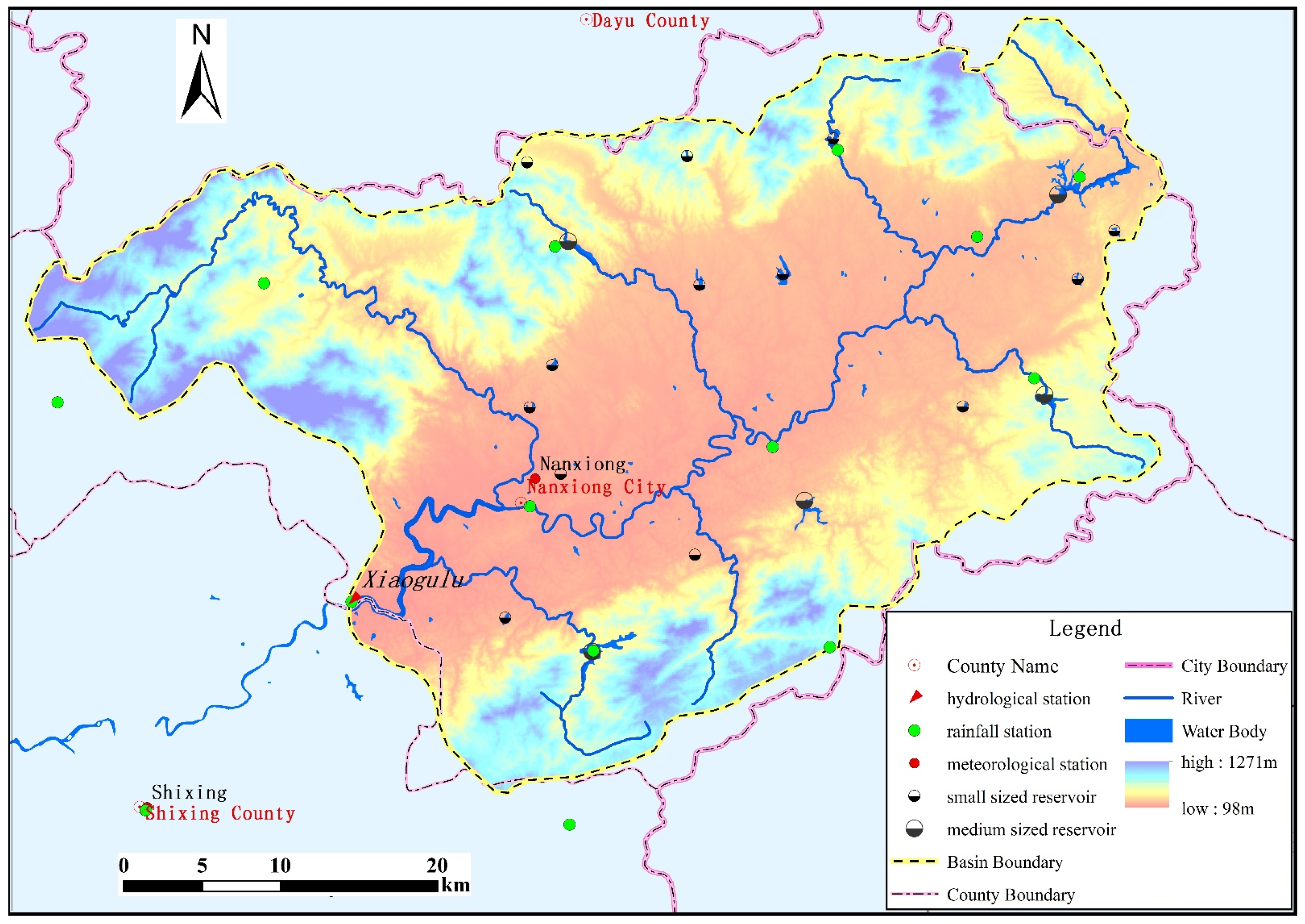
Zhenjiang River is upstream of the Beijiang River of the Pearl River system. The study area, with an area of about 1922.5 km
2, is the upper basin of the Zhenjiang River watershed above Xiaogulu hydrological station. It is a mountainous watershed, and the elevation of the study area ranges from 98 m to 1271 m; it is high in the elevation in the middle area from northeast to the southwest (mountains and hills) and low on both sides. It has low vegetation coverage in the Nanxiong basin, and the forest coverage rate is 64%, belonging to the area of soil erosion. There are 12 tributaries in this basin, with a total river length of 356.7 km. Xiaogulu hydrological station is located at the boundary line of Nanxiong City and Shixing County, Guangdong Province. From 2000 to 2013, the maximum peak flow of the Xiaogulu hydrological station was 1250 m
3/s. There are 5 medium reservoirs and 13 small reservoirs in the basin; the basic information of the 18 reservoirs can be seen in
Table A1 and
Table A2 of
Appendix A, but their operation data are not collected.
Figure 1 shows the DEM, river system, hydrometeorological stations, and reservoirs of the study area.
The watershed belongs to the subtropical monsoon climate area. The multi-year average temperature in the study area is 19.9 °C, the highest monthly average temperature is 28.8 °C, and the lowest monthly average temperature is 9.5 °C. The study area has abundant rainfall but uniform rainfall distribution: The average annual rainfall is about 1500 mm, and the average rainfall from May to October accounts for 66.9% of the annual average rainfall. The measured average annual evaporation of the Nanxiong meteorological station in the 30 years from 1981 to 2010 was 1066.2 mm (the evaporator was E601). The annual average runoff depth was about 782 mm, and the annual average sediment transport modulus was 245 t/km2.
The floods in the basin are formed by rainstorms, which mainly occur during the flood season from May to September. It has the characteristics of rainstorms and floods in small- and medium-sized mountainous watersheds—rapid concentration of flow, sharp rise and fall of the flood, high flood peak but small flood volume, wide coverage, and long duration. Most floods have single peaks or double peaks, and only a few floods have multiple peaks.
2.2. A Real-Time Flood Forecasting Method Based on the TOPKAPI Model
TOPKAPI is a fully distributed, physically based hydrological model with a simple structure and parameter scheme, which makes it one of the several operational distributed hydrological models in the world at present. It is also one of the core modules of the European Flood Forecasting System (EFFORTS). The latest model package consists of four parts—PreTPK, ITOPKAPI, TPKVIEW, and TPKMAPS. All stages, including the processing of DEM, the input of initial parameters, model operation, and graphical representation of the intermediate and final results, are completed in the same environment, which greatly improves the efficiency of data analysis and decision making of model application.
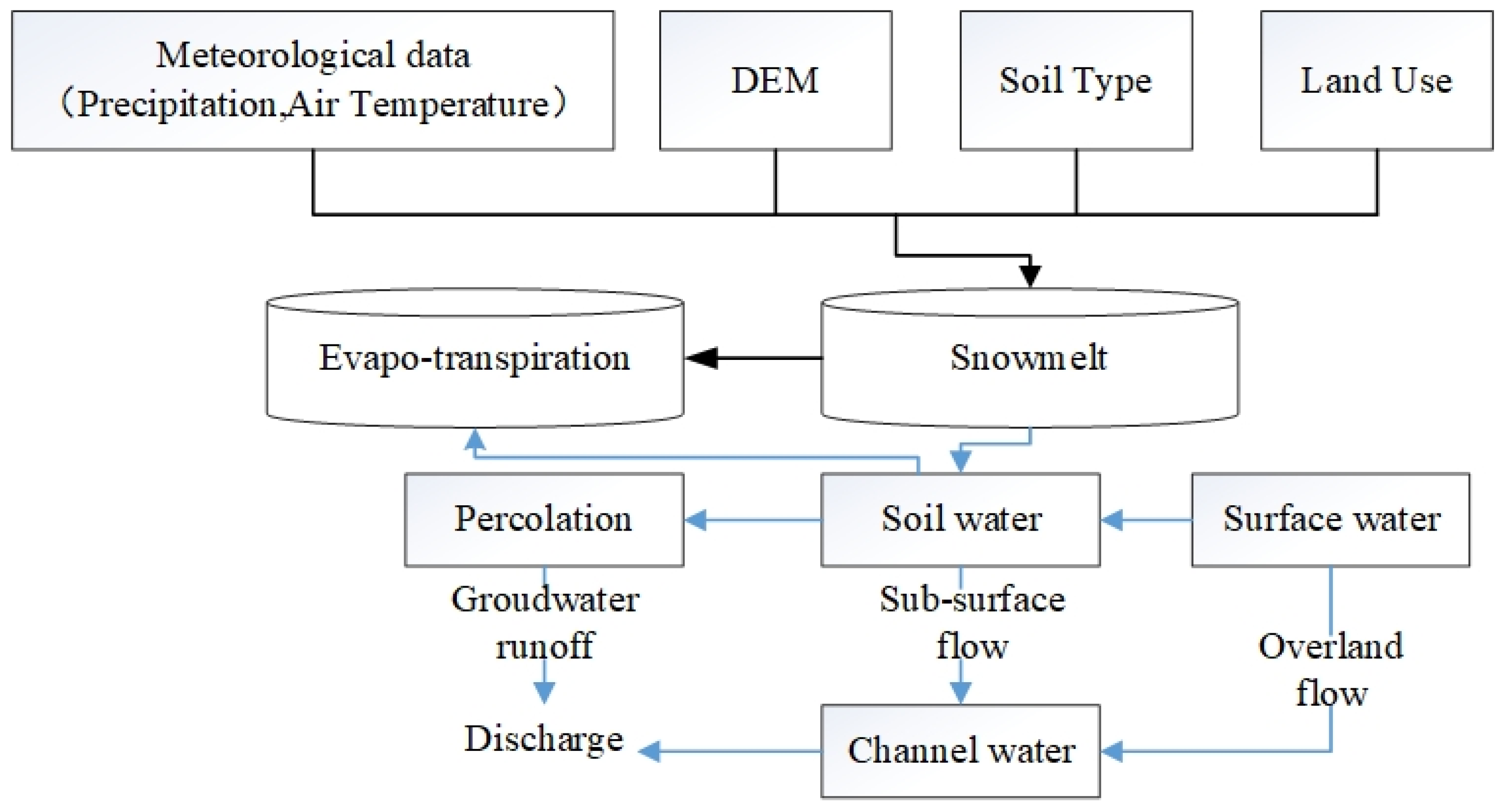
The model is generally divided into components of plant interception, snow melting, evapotranspiration, infiltration, percolation, surface flow, subsurface flow, underground flow, channel flow, reservoir/lake, and discharge. The model structure and simulation steps are shown in
Figure 2.
We used the software of Version 2.3 (released on 7 January 2016) of the TOPKAPI in this paper. The main characteristics of the model are as follows:
(1) It has reduced execution times suitable for distributed model calibrations and real-time operational applications and flood forecasting; (2) the model can be run at different time scales, from very fine temporal (few minutes) to daily simulations, and can resolve basin hydrologic response at spatial scales (100–1000 m) in both small and large catchments; (3) it can be easily calibrated due to physically meaningful parameters whose values can be retrieved from digital elevation maps, soil maps, land use, and vegetation maps, in terms of measurable physical quantities such as slope, soil permeability, surface roughness, etc.; (4) it tracks the spatial variability of runoff conditions in the catchment getting flow predictions at any point of the channel network (1D outputs) and explicitly considers the spatial variability in precipitation fields, fully exploiting distributed rainfall estimates such as the ones produced by RADAR networks [
23]; (5) it represents the behavior of the main components of the hydrological cycle, thus producing stream flow forecast, as well as distributed information on soil moisture, evapotranspiration, snow accumulation, etc. (2D output maps); (6) the TOPKAPI model can run independently offline, but also be used as a flood forecasting model in real-time flood operation system for continuous simulations or prediction calculation. It can be coupled with HEC–RAS hydraulic model (directly) or with Delft–SOBEK hydraulic model (via FEWS); (7) with the help of 3S technology, the model can be applied to the basin without data and can run basing events and continuously simulate different scenarios (water balance analysis, climate change, water resource condition change, etc.).
2.3. Materials
The application of the TOPKAPI model requires GIS data such as DEM, land use map, soil map, water system, maps of reservoirs/power stations and their physical attribute information, hydrological and meteorological data, and water resource utilization information of the basin. The specific process for the determination of its parameters can be seen in related studies or literature [
24]. In addition, in order to better calibrate the model, it also needs to understand and master the basin characteristics, hydrometeorology, historical flood characteristics, etc. Some basins may have weather radar rain data to input to make up for the lack of rainfall station data, such as time series of rainfall distribution map, which includes geographic location, spatial coverage, time, and spatial resolution of observation data.
2.3.1. DEM
DEM of the upper reaches of the Zhenjiang River in Guangdong Province was extracted from the GDEM data (
http://www.gscloud.cn/listdata/showinfo_new.Shtml?From=&id=304, accessed on 20 April 2020). After downloading the data and simple processing, the PreTPK interface can help the user to add the main rivers of the basin, set the minimum threshold value of the simulation area, and modify the DEM using the tools provided. Then, the DEM was converted into the data that can be directly used by the model, and the resolution was reduced to 500 m × 500 m (it can be set and modified according to the threshold of simulation area).
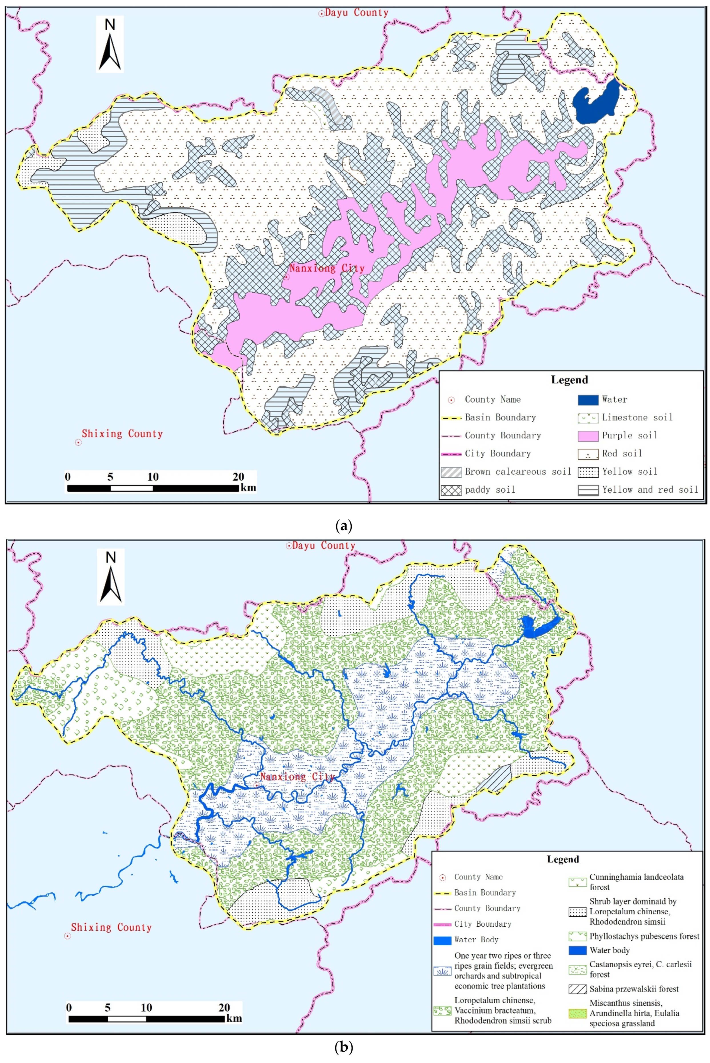
2.3.2. Soil Data
The soil map with the resolution of 1:1,000,000 was obtained from the website of the National Special Environment and Function of Observation and Research Stations Shared Service Platform (
http://www.ncdc.ac.cn/portal/metadata/navigator, accessed on 20 April 2020). There were 8 soil subclasses in the basin, and the names of each soil subclass are shown in
Figure 3a and
Table 1.
Red soil had the largest area in this basin, accounting for 50.96% of the basin area, followed by paddy soil, accounting for 24.27%, and purple soil, accounting for 12.64% of the basin area. These three soil subclasses were the main soil types in the basin. We queried the attribute information of each soil subclass needed by the model in the literature [
25,
26] and made a CSV type file named soil.csv to store these data. The file must have columns of data as follows: the first column was ID (vector of ID codes for soil types); the second column was DEPTH (vector of soil depth), followed by KSH (vector of hydraulic permeability (horizontal)), KSV (vector of hydraulic permeability (vertical)), THETA_R (vector of residual water content values), THETA_S (vector of saturation water content values), EXPH (vector of soil reservoir exponent), EXPV(vector of percolation law exponent), and NAME(vector of soil type names), respectively.
2.3.3. Vegetation
The land use map was obtained from the vegetation dataset of China with a resolution of 1:1,000,000. The vegetation types of the study area are shown in
Figure 3b.
The vegetation with the largest area in the basin was Loropetalum chinense, Vaccinium bracteatum, Rhododendron simsii scrub, accounting for 47.33% of the basin area, followed by double-cropping rice and orchards, accounting for 23.98%. We queried the initial value of the attribute information of each vegetation type required by the model in some studies in the literature [
27] and made it a CSV-type file named landuse.csv. The file must have columns of data as follows: the first column was ID (for vegetation types); the second column was the surface Manning coefficient of the land use type; columns 3–14 were the vegetation index of January to December, respectively. The index can be inquired in the irrigation and drainage literature of “vegetation water demand” of FAO.
2.3.4. Hydrometeorological Data
- (1)
Rainfall data and processing
The operation of the model requires a long series of continuous precipitation data (at least 5 years), and we collected the long series of precipitation data of 9 rainfall stations located in the basin. However, there was basically no precipitation data from December to March of the next year of all the rainfall stations.
We selected the forecast period as one hour and processed the precipitation data using the linear interpolation method. We set −9999 when there was no observed data from November to March of the next year. From 8:00 on 1 March 2000, the data of each rainfall station was written into a CSV type file named rainfall.csv, and one column for each station. At the same time, the location of these rainfall stations were written into a CSV file named rainfall.csv.xyz.
- (2)
Temperature data and processing
TOPKAPI needed temperature data, and there was only one meteorological station named Nanxiong in the basin. The daily average temperature, daily maximum temperature, daily minimum temperature data of the year from 2000 to 2013, and station location of Nanxiong meteorological station was obtained on China Meteorological Data Network (
http://data.cma.cn/site/index.html, accessed on 21 April 2020).
It needed the hourly temperature data to obtain the hourly model results; therefore, we converted the daily temperature into the hourly data according to the three characteristic temperature values of the daily average temperature, the daily maximum temperature, and the daily minimum temperature. First, we judged the temperature at a certain time should fall down between which two characteristic values. Then, the linear interpolation method was adopted to obtain the temperature of the time by using these two characteristic values and time intervals. It should be noted that this interpolation may have a deviation from the actual hourly data, and therefore, it is temporarily approximate.
We made a CSV-type file named tmp.csv according to the specified format. The file was more or less the same as rainfall.csv. Similarly, the location of the Nanxiong meteorological station was written into a file named tmp.csv.xyz. The monthly average temperature was also made into a CSV-type file named tmp_m.csv. The model used air temperature data to calculate evaporation, so evaporation data of the basin were not collected.
2.3.5. Flood Data
The flood data mainly refer to the long series flood element data (at least 5 years and the same period with rainfall data) of a hydrological station or water level gauges, the water-level–discharge curve of a forecast section, etc. In the study basin, only Xiaogulu hydrological station had a long series of water level and flow data, and the data of flood elements of the station (water level and flow from March to October) from 2000 to 2013 were collected.
The flood data of Xiaogulu hydrological station were available hour by hour but sometimes failed within the series; on such occasions, the flow would be changed into the hourly data using the linear interpolation method. Then, it was made into a CSV-type file named Qobv.csv according to the format required by the model input. The first two columns of the first line in the file were time and code, and the second line and later lines of the file were the corresponding values.
2.3.6. Other Data
The required water system map was mainly used to refine the drainage network generated by DEM, and that map with the resolution of 1:250,000 of the basin was collected. According to this map, the vector map of the basin boundary was drawn in the GIS software. There were 18 medium and small-sized reservoirs in the basin. According to the model, it needed geographic location, storage capacity curve, discharge curve, long series data of inflow/outflow, reservoir operation data of selected flood events, etc., but we had no data about them except their locations, so the reservoirs in the basin were not simulated, and it was treated as one basin with no reservoir. There was no large-scale external water transfer in and out of the basin, which was not considered in the simulation.
2.4. Model Implementation
The prediction scheme was made based on the river system, hydrological station data compilation, and flood characteristics analysis of the Zhenjiang River basin above Xiaogulu station. First, according to the general situation of the basin, the simulating period was selected, which was from 2000 to 2013, and the time step of the simulation was set to one hour. Then, the data required by the TOPKAPI model were collected and processed. Next, the model parameters were set and the model was run, after which 26 flood events whose peak discharge rates were more than 500 m3/s were selected according to the actual flood events of the basin, to calibrate, verify, and determine a group of optimal model parameters. Finally, the accuracy and prediction results were evaluated and analyzed.
2.5. Evaluation Indices
In this study, Error of peak discharge (
EPD), Nash efficiency coefficient (
E), mean absolute error (
MAE), root-mean-square error (
RMSE), coefficient of determination (
R2), explained variance (
EV), volume control index (
VC), Chiew and Mcmahon (
CMM), and index of agreement (
d) were selected as evaluation indices to analyze the simulation accuracy.
Table 2 lists the calculation formula of these evaluation indices.
3. Simulation Results
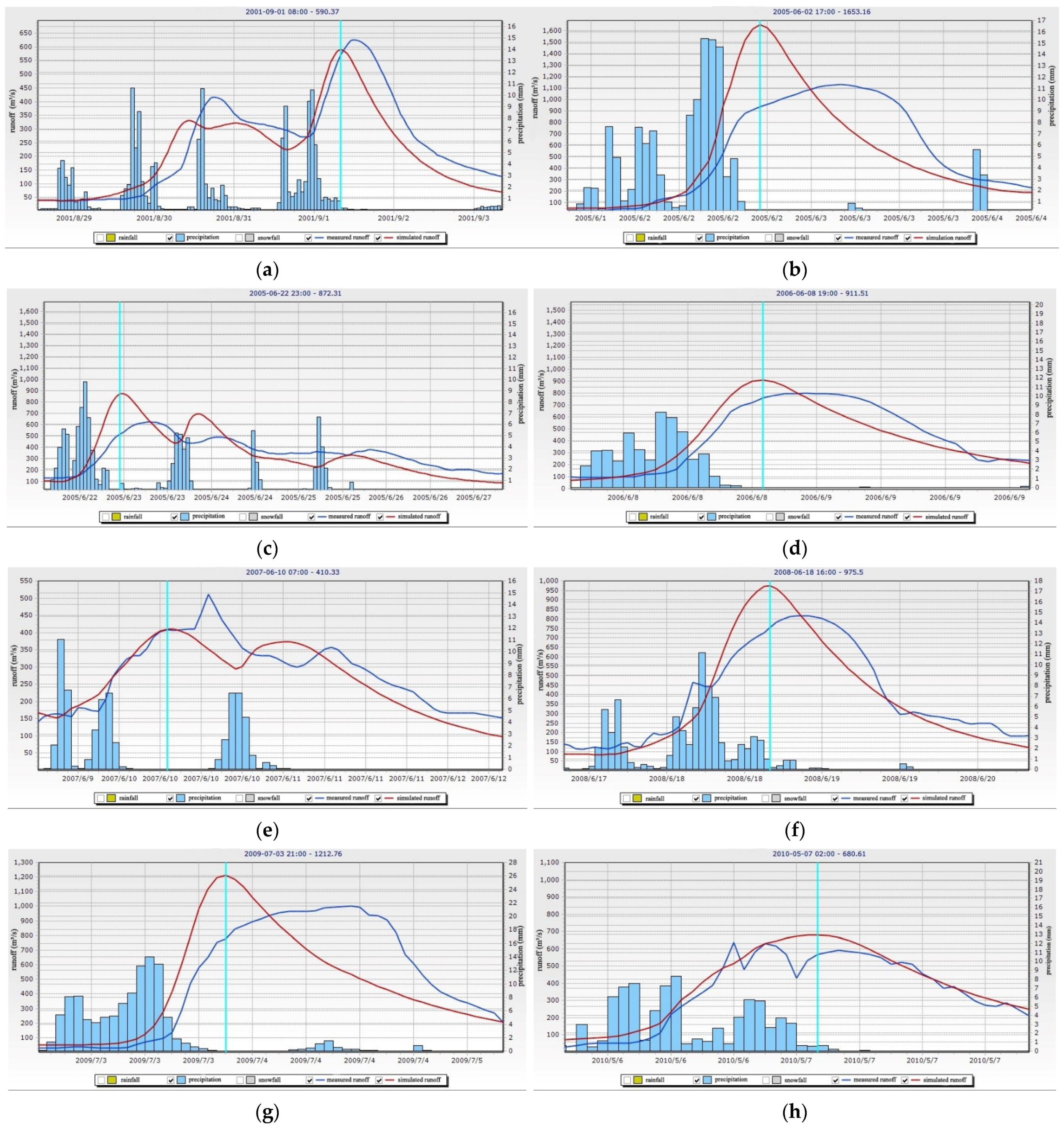
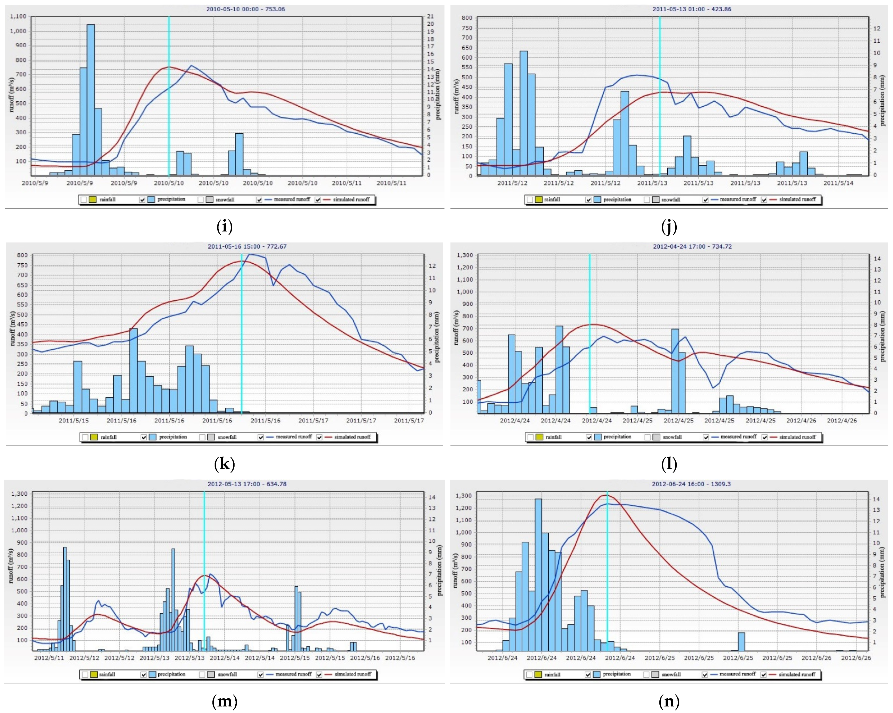
When all of the files were prepared and checked, they were used to run and calibrate the TOPKAPI model. Based on the calibrated parameters, the long series hourly simulation results of each year from 2000 to 2013 were obtained, and then, 26 selected floods with peak discharge rates greater than 500 m3/s were selected to analyze the simulation results of Xiaogulu station.
The TOPKAPI model does not need to divide the simulation period into calibration and verification periods, but according to the needs of model parameter calibration and verification, the first 18 floods were used to calibrate model parameters, and the last 8 floods were used to verify the parameters.
Table 3 shows the simulation results of 26 selected flood events. Considering the limit in the length of this article, only some selected flood simulation results are given below (
Figure 4).
According to the requirements of the standard for hydrological information and hydrological forecasting (GB/T22482-2008) [
28], the evaluation items of flood forecasting accuracy include flood peak discharge (or water level), flood volume (runoff), occurrence time of the flood peak, and process conformance of the flood event. When the flood peak discharge is used to evaluate the accuracy of the prediction scheme (the simulated flood volume in the TOPKAPI model was not calculated yet), the evaluation index is the error of peak discharge: When the pass rate is more than 85.0%, the accuracy class is Level A; when the pass rate is more than 70.0% and less than 85.0%, the accuracy class is Level B; when the pass rate is more than 60.0% and less than 70.0%, the accuracy class is Level C; otherwise, it failed to meet the standard.
Table 4 lists the accuracy evaluation results (weather up to the standard) of the TOPKAPI model of 26 selected flood events with peak discharge rates greater than 500 m
3/s, from April 2000 to November 2013.
Based on the test of the selected flood events with peak discharge rates of more than 500 m3/s, taking 20% of the peak discharge as the allowable error (EPD ≤ 20%), the prediction scheme of Xiaogulu station established by the TOPKAPI model had a simulation accuracy as follows: The pass rate was 66.67% in the calibration period and 75% in the validation period, which is Level C and Level B, respectively. In the whole simulation period, taking 20% of the peak discharge as the allowable error, the prediction accuracy was Level C.
When using the Nash efficiency coefficient (
E) as the evaluation index, the mean
E of the selected 26 flood events was 0.789, and the value of the Nash efficiency coefficient of 21 flood events was larger than 0.7 in the whole period. When using the coefficient of determination (
R2) as the evaluation index, the mean
R2 of the selected 26 flood events was 0.893, and the value of
R2 of 23 flood events was larger than 0.8 in the whole period. When using the index of agreement (
d) as the evaluation index, the mean
d of the selected 26 flood events was 0.918, and the value of
d of all flood events was larger than 0.8 in the whole period. Other results of evaluation indices can be seen in
Table 3.
4. Discussion
When using the indices of E, R2 and d as the evaluation indices, the simulation results are good, but using the EPD as the evaluation index, according to the requirements of the standard GB/T22482-2008, some flood events are failed to the standard, and at the same time, the simulated occurrence time of the selected flood events has deviation, too. Therefore, the forecast results using the calibrated parameters can only be used for estimation. In general, the reasons for the deviation between the simulated and observed peak discharge and its occurrence time of 26 flood events can be explained as follows:
(1) The regulation influence of small- and medium-sized reservoirs on the basin’s water storage: Since the operation data of these 18 reservoirs had not been collected, the water storage and drainage of these reservoirs had not been simulated and, therefore, these areas were treated as no reservoir in the basin. The total catchment area of these reservoirs was up to 324.04 km2, accounting for 16.86% of the study area. The five medium-sized reservoirs had regulation capacity, among which Hengjiang reservoir had multi-year regulation capacity. In the flood season, it can store and release water according to the predicted inflow, thus affecting the flooding process of its downstream basin.
Figure 4b,d,g reveal similar simulated and measured processes that floods might have undergone following the reservoirs’ storage and regulation.
Figure 4g can serve as an example for a simple analysis. Several rainfall stations with the largest rainfall in this flood event were located in the upper and middle reaches, and the total rainfall of Dayuan station with the largest rainfall (within 52 h) was 264.6 mm, and that of Nanpu station with the smallest rainfall is 28.9 mm. It was possible that through the storage of several reservoirs, the measured flood peak flow of Xiaogulu station would be cut off by about 20%, and the occurrence time of the peak would be delayed, according to the simulated results (regarding no reservoirs in the basin).
(2) Deviation in the processing of temperature, precipitation, and flow data: Since the hourly data of meteorological stations in the basin were not available, and only one meteorological station in the basin had daily temperature data, the hourly temperature data obtained from the daily average temperature, daily maximum temperature, and daily minimum temperature might have some deviation. Meanwhile, the hourly precipitation data would also have deviation when the precipitation lasted for a short time, but since it was evenly distributed to an hour, the rainfall intensity would be reduced, affecting the flood peak discharge. Similarly, the measured flow of the Xiaogulu station was processed into a one-hour period, and therefore, the hourly flow obtained by the linear interpolation method would also have some deviation.
Figure 4e,h,k, show the processing trace of linear interpolation of measured flow data; nevertheless, the simulated results of these flood events still met the standard.
(3) Deviation of soil and land use attribute information: As the detailed soil and land use attribute information in the basin required by the model was not collected, the same type of soil and land use attribute information in other regions was used instead. The spatial difference in different places was large. Although this aspect had been taken into account in parameter calibration, the deviation would still exist, especially in the parameters of soil thickness and hydraulic conductivity, and they would have some influence on the simulation results. Therefore, simulation results in the calibration period based on the normal range of calibrated soil attribute parameter values were not ideal, and the corresponding verification results were not satisfactory. The runoff recession process in
Figure 4a,c,e shifted to an earlier time, compared with the measured process, and this phenomenon might relate to the soil and land use parameters.
(4) The influence of rainstorm centers and the deviation of processing point rainfall into areal rainfall caused by rainfall non-uniformity: The average rainfall station density was 213.5 km2/station in this basin, but there was a considerable amount of rainfall in southern China, and the rainstorm center moved frequently, so relatively speaking, the rainfall stations were fewer, and the influence of processing point rainfall into areal rainfall could not be avoided.
(5) The reason attributed to the model itself and the impact of discontinuous rainfall and discharge data: The model is suitable for long series and continuous hydrological simulation. If the rainfall data were missing, the rainfall would be treated as 0, while if the temperature data were missing, the model would continue to calculate according to the monthly average temperature provided. The processing method of missing rainfall data would lead to lower simulated runoff. The model had a long preheating period (3–4 months or even longer) at the beginning of the simulation. In the case of only excerpted precipitation data from March to November were collected, the model had just been successfully preheated, but the precipitation data were interrupted again from November to March of the next year, so the model had to repeatedly preheat, resulting in some deviation between the simulated and the measured runoff. Since there were no rainfall and discharge data collected from November to March of the next year, when the model automatically read the data, the rainfall was treated as 0, resulting in inaccurate flood simulation values of March to May of each year, or even longer.
(6) Influence of initial state: In order to accelerate the preheating of the model, when setting the initial state of the soil, a larger percentage of monthly average saturated water content was set each month, and the same initial state was used in each year, which may be inconsistent with the actual situation.
5. Conclusions
Based on the simulation results and the discussion above, some suggestions are provided when using TOPKAPI in the study area and similar basins with reservoirs: (1) the operation data of medium-sized reservoirs in the basin, especially the water discharge of these reservoirs in case of large floods, should be collected; then, it should be recalibrated, and the model parameters, verified; (2) after collecting the hourly rainfall, temperature, flow, and evaporation data, the processing and integration of measured data need to be studied, to ensure the processing accuracy meets the requirements. Meanwhile, the quality of data used should be improved, with the aim to increase data collection and compilation quality in the dry season; (3) the attribute information of soil and land use and other data needed by the model in the basin need to be collected.
There are 5 medium-sized reservoirs and 13 small-sized reservoirs in this study area. Due to the lack of reservoir operation data, the model parameter calibration and validation can only be based on precipitation data and measured flow data, which increases the difficulty and inaccuracy of the model parameter calibration and flood process analysis. In practice, the real-time flood forecasting should be closely combined with the reservoir dispatching, especially withthe five medium-sized reservoirs in the basin. The soil moisture content of the early stage should be adjusted in real time, to obtain good results.


 ,
, 

