Research on Reservoir Optimal Operation Based on Long-Term and Mid-Long-Term Nested Models

Abstract

In order to solve the problem that the existing optimal operation model of reservoirs cannot coordinate the contradiction between long-term and short-term benefits, the paper nested the long-term optimal operation and mid-long-term optimal operations of reservoirs and established the multi-objective optimal operation nested model of reservoirs. At the same time, based on this model, the optimal control mode is determined when there are errors in the predicted runoff. In the optimal scheduling nested model, the dynamic programming algorithm is used to determine the long-term optimal scheduling solution, and the genetic algorithm is used to solve the mid-long-term optimal scheduling. The optimal control mode is determined by three indicators: power generation benefit, water level over limit risk rate and the not-exploited water volume. The results show that, on the premise of meeting the flood control objectives, the nested model optimal dispatching plan has higher benefits than the long-term optimal dispatching plan and the actual dispatching plan, which verifies the superiority of the nested model in the reservoir optimal dispatching problem. When there is error in predicting runoff, among the water level control mode, flow control mode and output control mode, the average power generation benefit of output control mode is 150.05 GW·h, the low-risk rate of water level overrun is 0.29, and the not-exploited water volume is 39,270 m³. Compared with the water level control mode and the flow control mode, the output control mode has the advantages of higher power generation efficiency, lower water level over limit risk rate and less not-exploited water volume. Therefore, from the perspective of economic benefit and risk balance, the output control mode in the optimization scheduling nested mode is the optimal control mode.

1. Introduction

As the basic material of human survival and development, water resources have the attributes of being the means of production and living resources on the one hand, and as a very important natural resource human life and economic construction on the other hand [1,2,3]. In the current situation of gradually increasing population and decreasing natural resources, and in the face of water shortage and frequent flood disasters, scholars have developed from the perspective of the rational utilization of water resources the goal of efficient and rational utilization of water resources [4,5,6,7]. As an important water supply source, the reservoir plays an important role in the utilization and allocation of water resources. Reservoir optimal scheduling is one of the most important means to efficiently utilize water resources, improve flood utilization, and increase reservoir benefits [8,9].

The classical solution method for reservoir optimization scheduling includes dynamic planning [10,11], linear planning [12], nonlinear planning [13], and large system decomposition and coordination methods [14]. With the continuous improvement of hydrological and rainfall and other related data, such as operations research [15,16], system engineering [17] and intelligent algorithms [18], reservoir optimization scheduling has developed rapidly.

Chen et al. [19] proposed the preferred decision principle and method of water resources system variable set optimization, which not only better coordinates the multiple benefits in the reservoir decision-making but also do so in a more reasonable manner. Zhang et al. [20] proposed to use cutting-edge long-term and short-term intelligent storage algorithms to coordinate the contradictions among optimal operation schemes of a reservoir at a monthly scale, daily scale and hourly scale, comparing their efficiency and resulting in solving the optimal operation problems of reservoirs with other primary intelligent algorithms, such as the support vector machine and the classical neural. In a preliminary study of the intelligent adjustment of reservoir scheduling decision-making, Li et al. [21] worked to solve the dimensional disaster problem of long-term random scheduling. Based on the description of the random process of incoming water, a long-term reservoir optimization scheduling model based on reinforcement learning theory was proposed by using the SARSA algorithm with models in machine learning, and at the same time by considering the Markov characteristics of the warehousing random variables. Through a greedy decision along with an approximation iteration, they adjusted the learning parameters to solve the approximate optimal sequence. The NSGAII-ANN algorithm proposed by Shokri et al. [22] integrates the Artificial Intelligence Neural Network (ANN) method with the non-dominant ranked genetic algorithm. It is applied to solve the reservoir dispatching and flood control problems. Ucler et al. [23] combined game theory with multi-objective fuzzy optimization, showing that the preferred decision better mines the comprehensive benefits of the reservoir; Tinoco et al. [24] used a long series of simulation comparison optimization methods to discuss the application effect of various reservoir scheduling schemes in Ecuador, and the results can provide a reference for the water resources scheduling management decision of the basin control reservoir, and provide optimization suggestions for the reservoir irrigation and drainage channels. Celeste et al. [25] used the linear storage capacity transfer method to assign the long-term (monthly) scheduling decision to the short-term (daily) scheduling decision, and found that the scheduling decision plan is consistent with the plan obtained from the actual measured daily runoff as the forecast data. Jiang et al. [26] constructed a multi-layer nested multi-dimensional dynamic programming algorithm, which enhanced the dynamic programming algorithm’s ability to solve the joint optimal scheduling problem of cascade reservoir groups, effectively improving the computational efficiency, and alleviating the multi-dimensional dynamic programming dimensional disaster problem. Liu et al. [27] proposed a bisection interpolation and chaotic nested search algorithm for the joint optimization and dispatch of cascade reservoirs. The results showed that the nested algorithm has simplified parameter configuration, high stability, good global optimization and high practicality value. Hammid et al. [28] made a comprehensive review of the implementation of optimal generation scheduling in hydraulic systems, pointing out that previous studies mostly focused on hydropower generation scheduling based on hydropower stations and reservoirs, and future research should focus on long-term, mid-long-term and short-term hydraulic scheduling issues. Avesani et al. [29] used Autoarimax and Benchmark models to simulate the seasonal management of reservoirs in alpine areas, and evaluated the impact of innovative econometric models to improve prediction accuracy on the optimization of short-term hydropower benefits. The results showed that the use of the Autoarimax model can significantly increase the revenue of the storage hydropower system over the use of the standard model. Ahmad and Hossain [30] proposed a collaborative optimization scheme for reservoirs on long-term and short-term scales with the goal of maximizing hydropower generation. The results show that the hydropower efficiency can be improved using the collaborative optimization method. At present, most studies on optimal operation are based on a single time scale such as annual scale, monthly scale or daily scale to optimize the solution algorithm, without the perspective of coordinating the long-term and short-term benefits of reservoirs. Therefore, this paper takes reservoir optimal operation as the theme and studies reservoir optimal operation from the perspective of coordinating long-term benefits and mid-long-term benefits.

As the premise of reservoir optimal operation, runoff prediction is mainly determined by hydrological information, but the hydrological process is very complicated, which inevitably brings many uncertainties to reservoir optimal operation. In recent years, scholars continue to explore the impact of uncertainty on reservoir operation benefits. Cassagnole et al. [31] studied the impact of short-term (7 days) flow forecasts with different qualities on reservoir management and revenue based on a conceptual method. The results show that the quality of forecasts can lead to certain economic losses and lead to some extreme management problems. Xu et al. [32], based on the available analysis results of ten-day runoff prediction, described the runoff in sections according to availability and established an optimization model for the ten-day dispatch plan of the two-stage Hengren Cascade Power Station. Stergiadi et al. [33] applied the End Point Blending Framework (EPB) to assess the impact of initial conditions and climate forcing on seasonal runoff forecasts in the basin, the results show that compared with traditional ESP/revESP method, EPB can identify sources of seasonal hydrological predictability based on watershed geology. Harrigan et al. [34] studied the relationship between catchment storage and Ensemble streamflow predictions (ESP) using a sample of 314 catchments in the UK, and the results showed that ESP can match climatology benchmark forecast in most catchments. Arsenault and Côté [35] investigated the effects of seasonal forecasting biases on hydropower management based on an ensemble streamflow prediction (ESP) approach, using historical precipitation and temperature time series to develop possible future climate scenarios and forcing hydrological models. The results showed that systems with stronger constraints tend to be more robust to prediction bias. Lamontagne and Stedinger [36] presented two statistical models to generate synthetic forecast values based on a time series of observed weekly flows. Mujumdar and Nirmala [37] aggregated individual inflows to reservoirs in cascaded hydropower systems by addressing forecast uncertainty and inflow uncertainty, and used Bayesian stochastic dynamic programming (BSDP) to represent the prediction uncertainty of aggregation inputs.

The key elements of this work are to establish a multi-objective optimal scheduling nested model for reservoirs, and to determine the optimal control mode when there are errors in the predicted runoff according to the uncertainty of the predicted runoff. This paper is summarized as follows: Section 2 briefly introduces the research area, the optimization scheduling nested model, and the main methods and indicators adopted in this paper. In Section 3, the engineering application of the optimization scheduling nesting model is carried out, and the optimization effect is analyzed. Then, according to three evaluation indexes, the optimal control mode of the optimization scheduling nesting model is determined under the condition of runoff prediction error. See Section 4 for the conclusions.

2. Materials and Methods

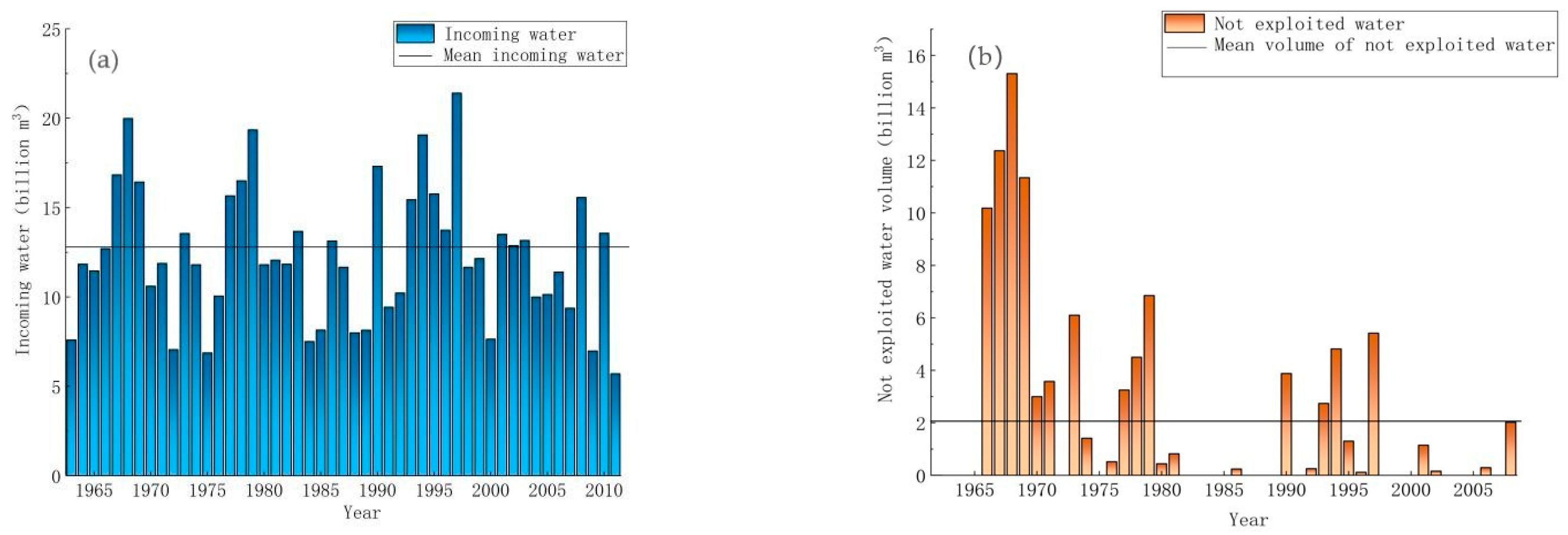
2.1. Data Sources

This paper will carry out research against the background of the reservoirs of southwest China, and the Chengbihe reservoir in Guangxi will be used for empirical research. Chengbi River reservoir is located in the lower reaches of Chengbi River, a tributary of Youjiang River, with power generation, flood control, fish farming, water supply and other comprehensive utilization functions. It is a large-type water conservancy project, with a total installed capacity of 30 MW. The reservoir has more than 50 consecutive years of hydrological and meteorological data from 1963 to 2014, with detailed data, which has the basis and conditions for empirical research.

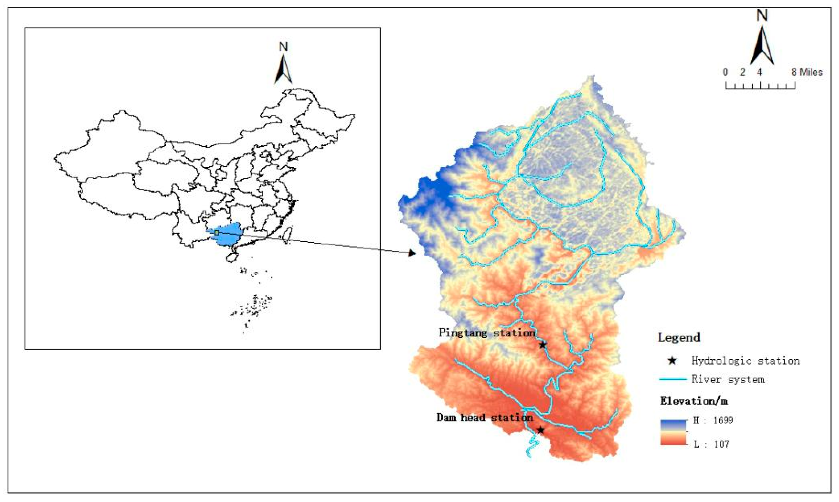
2.1.1. Basic Overview of the River Basin

Chengbi River originates from Taiyi Village, Yuhong Yao Township, at the north foot of Qinglong Mountain, Lingyun County, Guangxi. It is a first-class tributary of Youjiang River in the upper reaches of Yujiang River of Xijiang River system in the Pearl River Basin (Figure 1). The total area of the basin is 2087 km², of which the length of the main stream of the basin is 151 km, with an average drop of 3.87‰, an average elevation of 650 m and a total drop of 491 m.

2.1.2. General Situation of Chengbi River Reservoir Project

Chengbi River reservoir is located at the lower reaches of The Chengbi River, 7 km north of Baise City. The rainwater harvesting area above the dam site of the reservoir is 2000 km², accounting for 95.8% of the total basin area, among which the karst area is up to 400 km², accounting for about 20% of the rainwater harvesting area of the reservoir. It is a reservoir with multi-year regulation performance. According to the statistics of the inflow and not-exploited water of Chengbihe Reservoir over 49 years from 1963 to 2011 (Figure 2), it can be seen that the minimum inflow water of Chengbihe Reservoir from 1963 to 2011 was 7 billion m³, the maximum inflow water was 21 billion m³, and the average inflow water reached 12 billion m³. Meanwhile, the annual average amount of abandoned water in Chengbihe Reservoir was 2 billion m³ in 49 years, of which 26 years produced abandoned water. Based on analysis, 26 years account for 53.06% of the whole statistical period.

The capacity storage rate is the ratio of the actual storage capacity of Xingli storage and the designed storage capacity at the end of the flood season: the full storage rate of utilizable capacity from 1963 to 2011 of Chengbihe Reservoir (

Table 1. Chengbihe Reservoir capacity storage rate of Xingli Reservoir from 1963 to 2011.

Year	Capacity Storage Rate	Year	Capacity Storage Rate	Year	Capacity Storage Rate
1963	0.34	1980	1.03	1997	0.96
1964	0.59	1981	0.79	1998	0.94
1965	0.58	1982	0.70	1999	0.94
1966	0.48	1983	0.76	2000	0.41
1967	0.48	1984	0.52	2001	1.09
1968	0.22	1985	0.57	2002	1.13
1969	0.34	1986	1.05	2003	0.95
1970	0.76	1987	0.92	2004	0.84
1971	0.68	1988	0.76	2005	0.71
1972	0.53	1989	0.48	2006	1.02
1973	0.34	1990	1.01	2007	0.88
1974	0.83	1991	0.83	2008	1.01
1975	0.57	1992	1.03	2009	0.84
1976	0.81	1993	1.00	2010	0.80
1977	0.99	1994	1.00	2011	0.34
1978	0.89	1995	0.99
1979	0.87	1996	0.96

). Combined with the inflow and not-exploited water of Chengbihe Reservoir, it can be seen that the inflow water of Chengbihe reservoir was relatively abundant during the 49 years from 1963 to 2011, but flood resources were not fully utilized. The current operation mode failed to make full use of storm flood resources, resulting in a large amount of not-exploited water. As a result, the reservoir was filled up only 8 years out of 49 years, and the full storage rate was only 18.36%.

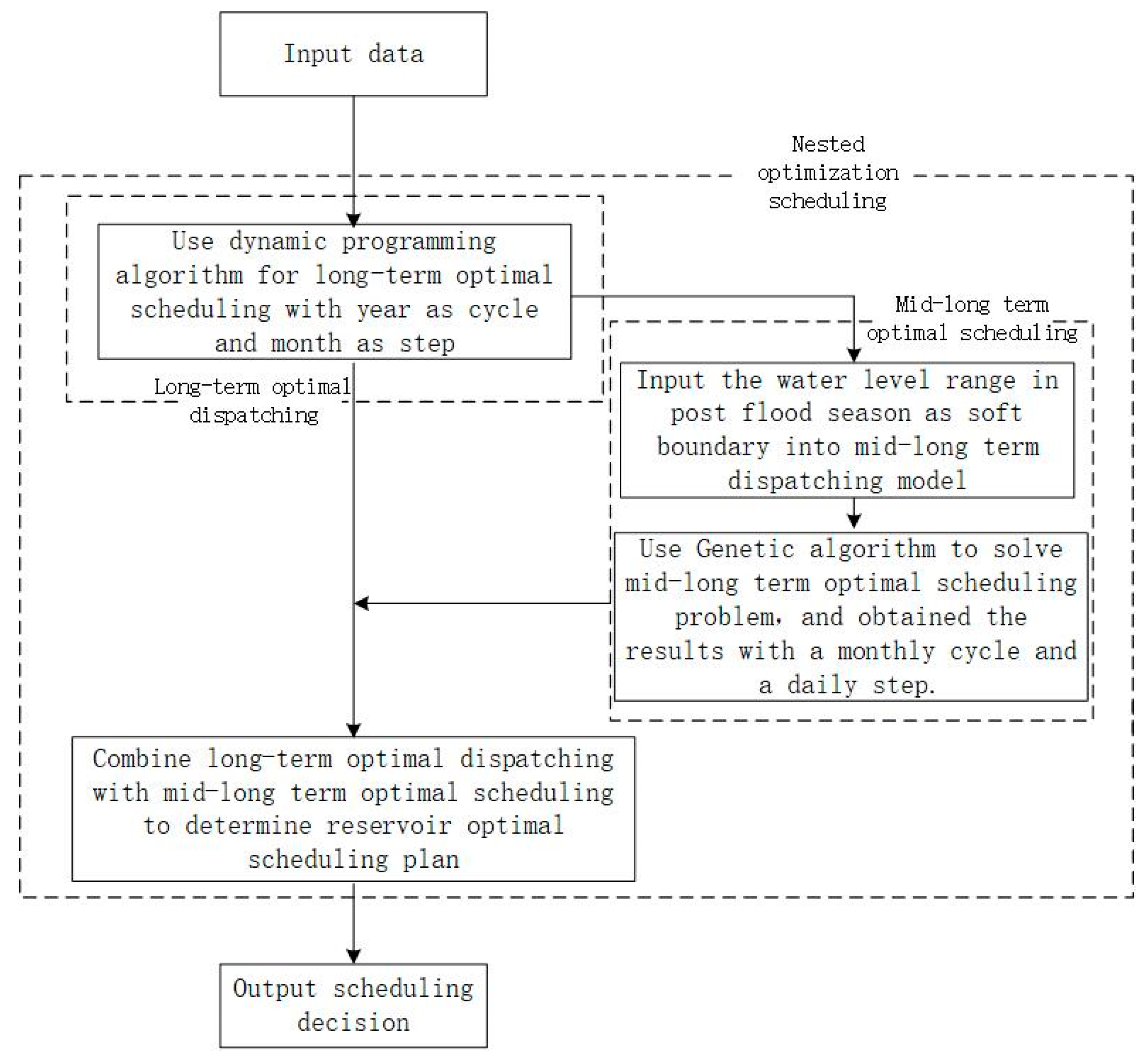
2.2. Optimization Scheduling Nested Model

2.2.1. Optimize Scheduling Nested Model Concept

In terms of scheduling models, optimization scheduling model can be divided into implicit stochastic optimization model, explicit stochastic optimization model and parameter simulation optimization model [38,39]. Each model has its own advantages and disadvantages in the simulation mode of scheduling information, solving efficiency and applicability. Among them, the Parametric simulation optimization model for could describe the uncertainty of hydrological sequence and forecast, coupled to a variety of prediction models for rolling real-time scheduling, can excavate potential reservoir scheduling. At present it has become the preferred form of scheduling model construction in most studies [40]. So, this paper build parameters optimization model for research of reservoir optimal operation.

Considering the coordination relationship between long-term and short-term benefits of reservoirs, an optimal operation model nested long-term and mid-long-term optimal operation is established. Macroscopically, from the perspective of the full cycle, the long-term optimal operation takes the long-term runoff forecast data as input, combined with the reservoir long-term operation plan and basic constraints, and determines the operation boundary of each time node in the full cycle, such as the key information of the end water level of the period, the discharge of the period and the inflow of the period. Microscopically, the decision set of the long-term optimal scheduling time period is transferred to the mid-long-term optimal scheduling model, and the range is taken as the soft boundary condition embedded in the mid-long-term optimal scheduling model, and the average daily runoff is taken as the scheduling basic data to solve the mid-long-term optimal scheduling decision range, and the optimization scheduling of different time scales is embedded. Since the update frequency of mid-long-term optimal scheduling decision is higher than that of long-term optimal scheduling decision, when extreme events cause a large deviation between the probability range of mid-long-term decision-making plan, the long-term plan will be updated and reset based on the mid-long-term optimal scheduling decision plan. In this paper, the nesting of optimal scheduling is only undertaken in flood season.

2.2.2. The Objective Function

In order to ensure the flood control and profit of the reservoir, the constraint method [41,42] is adopted to convert the flood control target into rigid constraint, and on the premise of meeting the flood control requirement, the multi-objective problem is transformed into a single-objective problem to maximize the power generation. The objective function of long-term optimal scheduling and mid-long-term optimal scheduling is expressed as follows:

$$E_{CQ}=\max {\displaystyle {\displaystyle \sum }_{t_1=1}^{T_1}K\cdot q_{e{t}_1}\cdot H_{t_1}}\cdot \nabla t_1$$

(1)

$$E_{ZQ}=\max {\displaystyle {\displaystyle \sum }_{t_2=1}^{T_2}K\cdot q_{e{t}_2}\cdot H_{t_2}}\cdot \nabla t_2$$

(2)

where $E_{CQ}$ and $E_{ZQ}$ are, respectively, the total energy generation under long-term optimal scheduling and the total energy generation under mid-long-term optimal scheduling, GW·h; $K$ is the efficiency coefficient of the reservoir; $T_1$ and $T_2$, respectively, represent the total number of scheduling periods based on year and month.

2.2.3. Constraint Condition

(1)

Water balance equation

$$V_i=V_{i-1}+(q_i-Q_i-q{s}_i)\cdot T_i$$

(3)

(2)

Capacity constraints

$$V_{\min }\le V_i\le V_{\max }$$

(4)

(3)

Water level constraints

$$Z_{\min }\le Z_i\le Z_{\max }$$

(5)

(4)

Lower discharge constraint

$$Q_i\le Q_{\max }=Q_f$$

(6)

(5)

Output constraints

$$N_{\min }\le N_i\le N_{\max }$$

(7)

where $V_{i-1}$ and $V_i$ are, respectively, the water storage capacity of the reservoir at the beginning and end of time, m³; $q_i$, $Q_i$ and $q{s}_i$ are, respectively, the reservoir inflow flow, power generation flow and lower discharge flow of the first period, m³/s; $V_{\max }$ and $V_{\min }$ are the lower limit and upper limit of the reservoir water storage at the end of the period, m³. In the long-term power generation scheduling, $V_{\min }$ is generally the dead storage capacity. In the flood season, $V_{\max }$ represents the storage capacity corresponding to the flood limit water level, and in the dry season, $V_{\max }$ represents the storage capacity corresponding to the normal water level. In the mid-long-term scheduling, the storage capacity in the post-flood season determined by the long-term scheduling is used as the boundary. $Z_{\max }$ and $Z_{\min }$ are the highest and lowest water levels allowed by the reservoir, m. In long-term scheduling, $Z_{\max }$ is generally taken the flood limit water level during the flood season, and it is taken the normal storage water level during the dry season, and $Z_{\min }$ is generally taken the dead water level. In the mid-long-term scheduling, the post-flood season water level determined by the long-term scheduling is used as the boundary for constraints; $Q_{\max }$ is the upper limit of discharge under the reservoir, m³/s; $N_{\max }$ and $N_{\min }$ are, respectively, the maximum and minimum outputs of the power station, kW.

Equations (3)–(7) are taken as constraint conditions of the objective function, and the nested model of reservoir optimal operation is constructed together with the objective function. It should be noted that the corresponding parameters of long-term optimal scheduling and mid-long-term optimal scheduling should be distinguished in the calculation. In the mid-long-term optimal scheduling, the water level and storage capacity in post-flood season determined by long-term optimal scheduling are taken as the boundary.

2.2.4. Model Solving Method

Model solving techniques can be divided into two categories: one includes deterministic optimization algorithms such as linear programming [43], mixed integer programming [44] and dynamic programming [11,45]; the other includes intelligent optimization algorithms such as genetic algorithm [46], annealing algorithm [47,48] and particle swarm optimization algorithm [49]. The two types of methods have their own applicability when solving scheduling models with different temporal-spatial scales and constraints. For example, the deterministic optimization algorithm should be used for solving long-term optimal scheduling decision scheme, while the intelligent optimization algorithm should be used for solving long-term and short-term optimal scheduling decision scheme [50].

Due to the different characteristics and adaptive models of the solution methods of the decision scheme, different algorithms are used to solve the long-term optimal scheduling and mid-long-term optimal scheduling in the nested optimization scheduling model. Dynamic programming algorithm belongs to deterministic optimization algorithm and is suitable for solving long-term optimal scheduling decision. It is advisable to adopt intelligent optimization algorithm to solve medium and long-term optimal scheduling decision scheme, while genetic algorithm belongs to intelligent optimization algorithm and is a global optimization method based on simulated biological evolution and natural selection mechanisms. Due to its advantages of simple operation and strong robustness, it is widely used in water resource optimization problems [51]. Therefore, this paper takes the dynamic programming method as the solution method of long-term optimal scheduling decision, and genetic algorithm as the solution method of mid-long-term optimal scheduling decision. The flow chart of optimization scheduling nested model (Figure 3).

2.3. The Evaluation Index

The existence of runoff prediction error is one of the important reasons for the difference in the implementation of control mode. Three indicators of hydropower station operation are calculated and compared when there is error in runoff prediction, and the influence of different implementation modes on the operation of hydropower station is analyzed. The three control modes of water level, flow rate and output are evaluated by three indexes: power generation benefit, water level over-limit risk rate and not-exploited water volume [52].

(1) Power generation benefit: Power generation benefit is an important evaluation index to evaluate the economic benefit in the operation of hydropower stations. It is determined by the energy generation during the scheduling period and energy storage at the end of the dispatch period. If the initial energy storage of the power station is certain, energy storage at the end of the dispatch period is represented by the increase of energy storage in the operation period. The specific calculation formula of power generation benefit is as follows:

$$B={\displaystyle {\displaystyle \sum }_{t=1}^T{N}_t\Delta t+{\displaystyle {\displaystyle \sum }_{t=1}^T\lambda (I_t-Q_t)\Delta t}}$$

(8)

where $B$ is the power generation benefit of hydropower station; $N_t$ is the output of the power station during the time period; $I_t$ is the inflow flow of the reservoir during the period; $Q_t$ is the outbound flow of the period; $T$ is the scheduling period; $\Delta t$ is the length of calculation period; $\lambda$ is energy efficiency coefficient of power station.

(2) Water level over-limit risk rate: Water level over-limit risk rate is an important index to measure the safety and stability of the reservoir. It is the proportion of the water level over limit period to the total period of operation period, and consists of water level over upper limit rate and water level over-lower limit risk rate. The calculation formula of water level overlimit risk rate is as follows:

$$R=R_u+R_d={\displaystyle {\displaystyle \sum }_{t=1}^T{r}_{u,t}+}{\displaystyle {\displaystyle \sum }_{t=1}^T{r}_{\mathrm{d},t}}$$

(9)

where $r_{u,t}$ and $r_{u,t}$ can be calculated by the formula. The calculation formula is as follows:

$$r_{u,t}=\{\begin{array}{ll}1/T& Z_t>Z_{\max }-\alpha ;A_{2,t}>0\\ 0& \mathrm{other}\end{array}$$

(10)

$$r_{d,t}=\{\begin{array}{ll}1/T& Z_t<Z_{\max }-\alpha ;Q_t<Q_{plan,t}\\ 0& \mathrm{other}\end{array}$$

(11)

where $R$ is the water level exceedance rate; $R_u$ is the upper limit rate of water level crossing; $R_d$ is the lower limit rate of water level crossing, $r_{u,t}$ and $r_{\mathrm{d},t}$ are the upper and lower limit functions of water level crossing, $\alpha$ is reserved water level, and $A_{2,t}$ is the second type of abandoned water amount during the power station period; $Q_{plan,t}$ is planned outbound traffic for the scheduling scheme.

(3) Not-exploited water volume: Not-exploited water volume refers to the part of the water that is wasted without producing any benefits during the reservoir operation period. The larger the volume of not-exploited water, the greater the loss of water energy. Therefore, the smaller the volume of not-exploited water, the better. It is a comprehensive evaluation index to measure the economic benefits and safety and stability of hydropower stations, including the first type and the second type of not-exploited water. Among these, the first type of not-exploited water refers to the not-exploited water that needs to be controlled when the water level has not reached the upper limit. The second type of not-exploited water refers to the not-exploited water generated in order to ensure the safety of the dam and prevent the water level from continuing to rise when the actual incoming flow is much larger than the predicted incoming flow. The formula for calculating the not-exploited water volume is:

$$L=L_1+L_2={\displaystyle {\displaystyle \sum }_{t=1}^T{A}_{1,t}\Delta t}+{\displaystyle {\displaystyle \sum }_{t=1}^T{A}_{2,t}\Delta t}$$

(12)

where L is the volume of not-exploited water; $L_1$ and $L_2$ are type I abandoned water and type II not-exploited water, respectively.

3. Results and Discussion

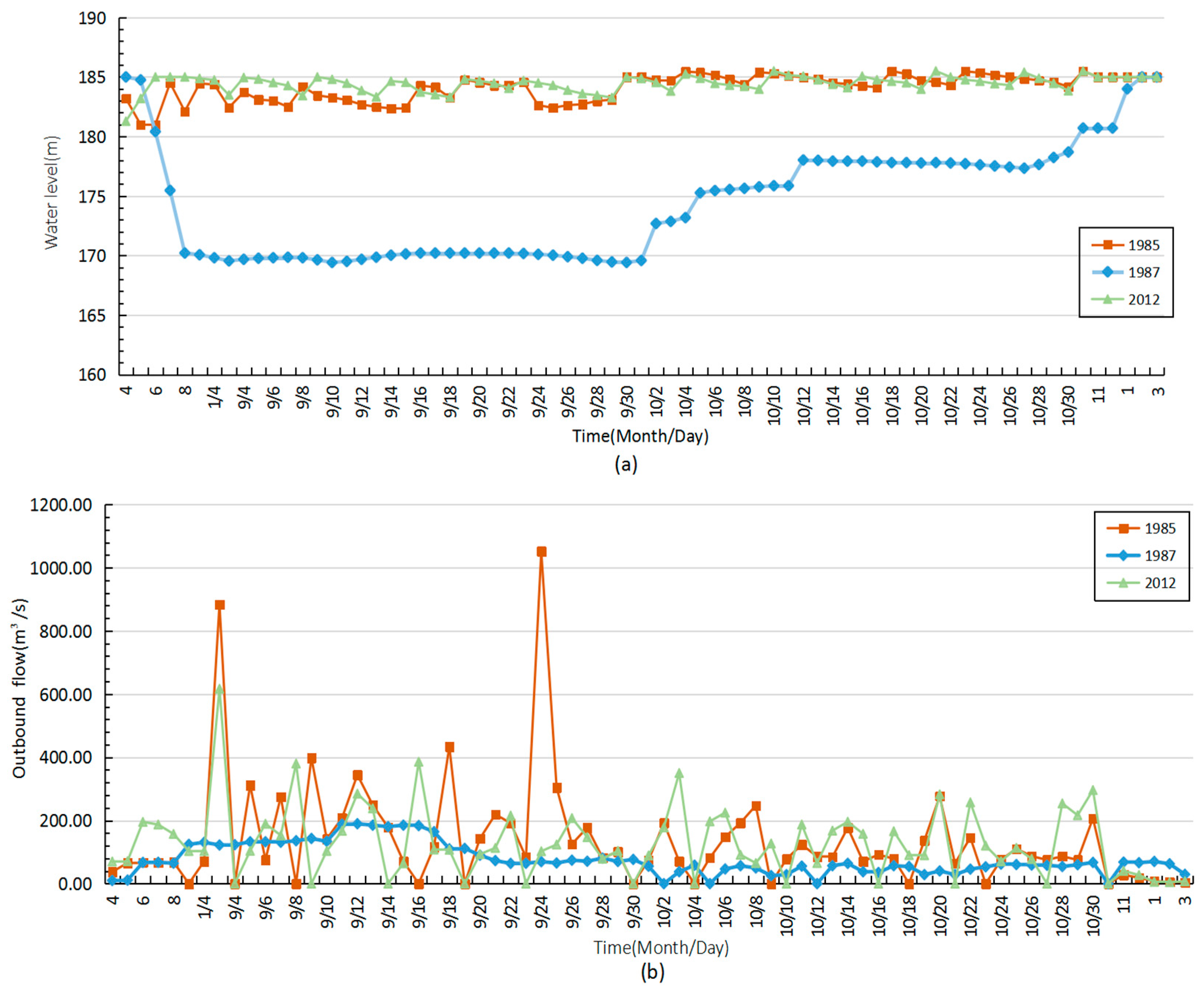
3.1. Application Results of Nested Optimization Scheduling Model in Typical Years

In this paper, hydrologic frequency analysis method [53] was used to determine the typical years. The P-III fitting line [54,55] was used for the average daily flow data from 1963 to 2014 at Dam head station of Chengbi River, and the hydrological years with guarantee rates of 25% (1985), 50% (1987) and 75% (2012) were selected as the typical years with abundant, flat and dry conditions. After determining the typical year, the actual inflow flow in the typical year was input into the model for calculation, and the calculation results of water level control and flow control in 1985, 1987 and 2012 were obtained (Figure 4).

At the same time, the typical annual inflow flow was input into the long-term optimal dispatching model. According to the calculation results of the nested optimization dispatching model and the long-term optimal dispatching model, the Chengbihe reservoir was simulated to calculate the power generation in 1985, 1987 and 2012. Combined with the annual energy generation of actual scheduling, the energy generation after simulation scheduling based on different scheduling schemes in typical years was counted (

Table 2. Comparison table of typical annual power generation under different scheduling modes (Unit: GW·h).

Year	Scheduling Model	1–3	9	10	11–12	Total
1985 (Dry)	Actual dispatch	46.02	8.36	8.15	13.91	110.50
	Long-term optimal scheduling model	106.36	21.95	7.71	16.05	152.07
	Optimal scheduling nested model	106.36	18.00	18.00	16.05	158.41
1987 (Flat)	Actual dispatch	80.39	7.40	12.31	21.77	121.86
	Long-term optimal scheduling model	122.17	16.76	19.29	43.35	194.63
	Optimal scheduling nested model	122.17	20.16	20.88	43.35	206.56
2012 (Abund)	Actual dispatch	63.45	13.09	8.83	18.07	103.44
	Long-term optimal scheduling model	120.49	8.07	5.58	23.34	157.48
	Optimal scheduling nested model	120.49	18.00	17.28	23.34	179.11

). The power generation comparison diagram was drawn under different scheduling schemes in typical years (Figure 5).

The power generation under each dispatch scheme in typical years is as follows: the power generation based on the optimal scheduling nested model is the largest, followed by the long-term optimal scheduling model, and the actual dispatch scheme is the smallest (Figure 5). As can be seen from Table 2, when the decision scheme based on the long-term optimal dispatching model and the optimal dispatching nested model is used to simulate the dispatching of Chengbihe Reservoir, the annual power generation generated during the dry year (1985) is 158.41 GW·h and 152.07 GW·h, respectively, increasing by 43.36% and 37.61% compared with the current scheme. In normal water year (1987), the annual power generation is 206.56 GW·h and 194.64 GW·h, respectively, increasing by 69.50% and 59.72% compared with the current scheme. In the wet year (2012), the annual power generation is 179.11 GW·h and 157.48 GW·h, figures which are increased by 73.16% and 52.25%, respectively compared with the current scheme. When scheduling according to the decision scheme of the optimal scheduling nested model, the annual power generation generated by scheduling has an increase rate of 5.74% to 20.91% compared with the long-term optimal scheduling scheme.

Further analysis of the annual power generation of each scheduling model shows that the scheduling scheme solved by the nested model generates more power generation in September and October compared with the long-term optimal scheduling scheme. The reason is that the scheduling scheme changes in September and October. In September and October, the mid-long-term optimal scheduling is embedded. The scheme in this period takes the water level at the beginning and end of the month determined by the long-term optimal scheduling as the soft boundary, and the scheduling decision is made according to the monthly predicted incoming flow with a daily step. The long-term optimal scheduling takes long-term benefits as the goal to make a global overall plan, while the mid-long-term optimal scheduling focuses on short-term benefits. Therefore, compared with the long-term optimal operation scheme, the optimal operation scheme solved by the nested model firstly aims at the maximum annual power generation, and then conducts the medium and long-term optimal operation in September and October, which can effectively coordinate the long-term and short-term benefits of the reservoir, avoid losing one to the other, and significantly improve the power generation of the reservoir.

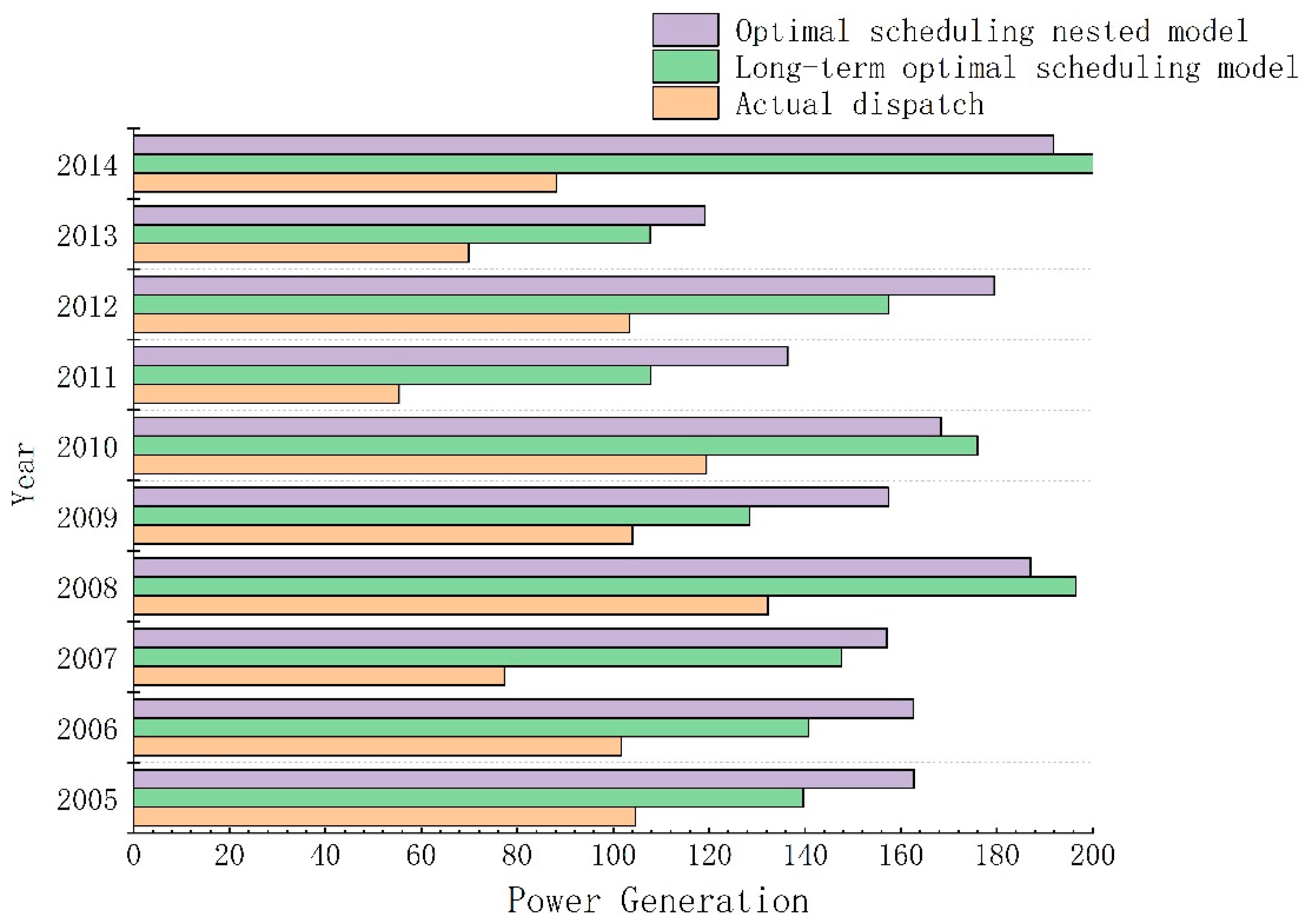
3.2. Application Results of Optimal Scheduling Nested Model from 2005 to 2014

In order to fully verify the effect of optimal dispatching nested model on power generation, the incoming flow of nearly ten years (2005–2014) was input into nested model and long-term optimal dispatching model, and the annual power generation of different dispatching models was counted (Figure 6). It can be seen that in the decade from 2005 to 2014, the power generation generated by optimal dispatching nested model was the highest except in 2008 and 2014. Compared with the long-term optimal operation model, it is reduced by 9.83 GW·h and 10.02 GW·h, respectively, which shows that the nested model of optimal operation has a certain universality for the improvement of reservoir power generation.

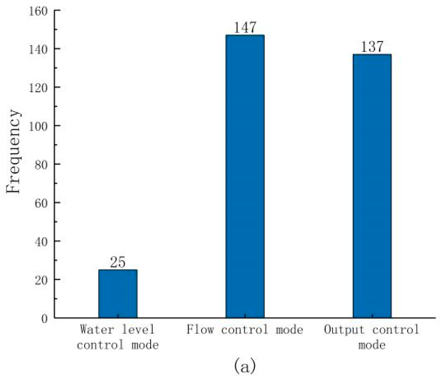
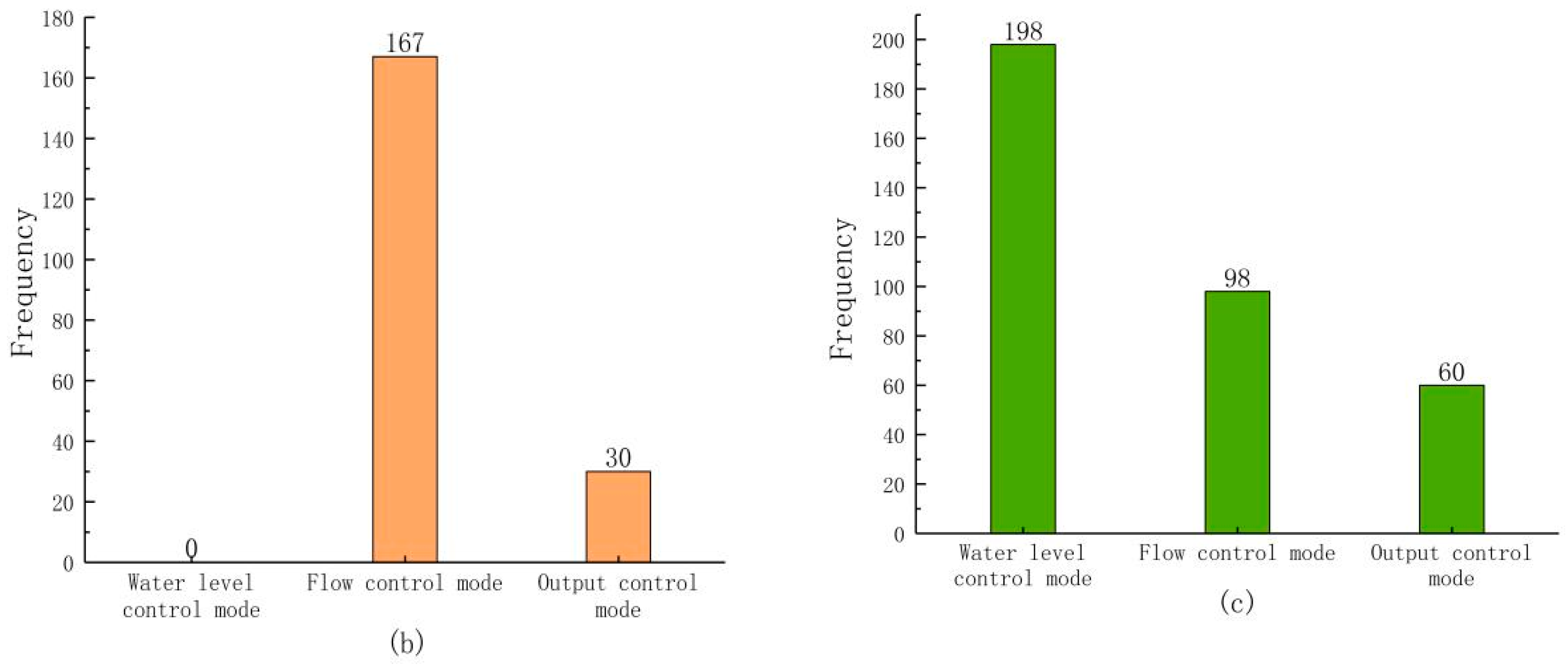
3.3. Comparison Results of Evaluation Indexes of Three Different Control Modes

The Monte Carlo method [56] was used to generate 300 error sequences with an average error rate of 5%, 10% and 15%, and then the actual inflow runoff from 2005 to 2014 was disturbed to generate 300 sets of predicted runoff with different errors. After 300 groups of 2005–2014 predicted runoff input optimization operation nested models, the control modes of water level, discharge and output in the reservoir operation process were determined Z = {$Z_1,Z_2\cdots Z_T$}, Q = {$Q_1,Q_2\cdots Q_T$}, N = {$N_1,N_2\cdots N_T$}, and then the average daily inflow runoff of Chengbihe reservoir from 2005 to 2014 was taken as the actual inflow runoff to simulate the operation. The three evaluation indexes of power generation benefit, water level over-limit risk rate and not-exploited water volume under different control modes were calculated [52], and the influence of uncertain incoming flow on different control modes was analyzed.

3.3.1. Qualitative Analysis of Evaluation Indicators

Count the times that 300 groups of predicted runoff power generation benefits and not-exploited water volume reach the maximum value and the times that water level exceeds the limit under three different control modes (Figure 7). It can be seen from (Figure 7a) that the power generation benefits of the three control modes are as follows: the water level control mode achieves the maximum power generation benefits for the least times, only 25 times, the flow control mode 147 times, and the output control mode 137 times. It can be seen from (Figure 7b) that the water level exceeding limits of the three control modes are as follows: water level exceeding limits does not occur in the water level control mode during the observation period, water level exceeding limits occasionally occurs in the output control mode, and water level exceeding limits occurs 167 times in the flow control mode. Further analysis of the performance of abandoned water in the three control modes shows that, as shown in figure (Figure 7c), the not-exploited water volume in the water level control mode is higher than that in the other two control modes, with a total of 198 times reaching the maximum value, followed by the flow control mode and the output control mode, which are 98 times and 60 times, respectively.

It can be seen that the flow control mode has the best power generation benefit, but the water level over limit risk rate in the flow control mode has occurred 167 times in total, and this control mode brings higher risk to the reservoir than the other two modes. The water level control mode has the lowest water level over limit risk rate, which can effectively ensure the safety of the dam, but the water level control mode has the lowest power generation benefit and the largest volume of not-exploited water, failing to make full use of water resources. In the output control mode, the volume of not-exploited water is the smallest, and the power generation efficiency is higher, and only occasionally the water level exceeds the limit.

3.3.2. Quantitative Analysis of Evaluation Indicators

In order to quantitatively analyze the size of evaluation indexes under different modes, the average values of power generation benefit, water level overlimit risk rate and not-exploited water volume under 300 working conditions were counted (

Table 3. Comparison table of the mean values of evaluation indexes of different control modes.

Control Modes	Power Generation Benefit (GW·h)	Water Level Over-Limit Risk Rate	Not-Exploited Water Volume (Millions of m3)
Water level control modes	149.28	0.00	39,786
Flow control modes	151.39	0.29	39,852
Output control modes	150.05	0.01	39,270

). The analysis shows that the maximum average power generation benefit is 151.39 GW·h under flow mode, while the power generation benefit is slightly reduced to 150.05 GW·h under output mode, and the lowest power generation benefit is 149.28 GW·h under water level control mode. In the water level control mode, there is no water level over limit risk, and the average over limit rate is 0. In the output control mode, the water level over limit risk rate is less, and the average over limit rate is 0.01. In the flow control mode, the water level over limit risk rate is very high, and the average over limit rate is 0.29. Water level control mode has the largest volume of not-exploited water, with an average of 39,852 million m³, followed by flow control mode and output control mode, with an average of 39,786 million m³ and 39,270 million m³, respectively.

In conclusion, the water level control mode does not exhibit the risk of water level exceeding the limit, but its power generation benefit is the worst due to the largest volume of not-exploited water generated. The flow control mode has the highest power generation benefit, but the risk rate of water level exceeding the limit is also the highest in the case of the uncertainty of incoming flow prediction. Compared with flow control mode, the average power generation benefit of output mode is only reduced by 1.34 GW·h, the risk rate of water level crossing is low, and the average volume of not-exploited water is the lowest among the three control modes. Therefore, from the perspective of economic benefit and risk balance, it is not recommended that the water level control mode and flow control mode be used as the control mode of reservoir operation, and that the output control mode be the optimal control mode of hydropower station operation.

4. Conclusions

Optimal reservoir operation is one of the important means to efficiently utilize water resources and increase reservoir benefits. However, at present most reservoir operation decisions cannot fully consider the coordination between long-term and short-term benefits of the reservoir, because short-term benefits are obtained but long-term benefits are ignored. Therefore, the purpose of this study is to set up a nested model of reservoir multi-objective optimal operation by nesting the long-term optimal operation and mid-long-term optimal operation with the goal of flood control and profit. After the Scheduling model is established—three typical years of Abund, Flat and Dry— nearly 10 years of data (2005–2014) from the incoming runoff input nested optimization scheduling model is used to obtain the optimal scheduling scheme after simulated scheduling. With the current scheduling scheme and only the long-term optimal scheduling scheme contrast, the efficacy of the optimization scheduling of nested model optimization is evaluated. Then, according to the scheduling decision of the optimal scheduling nested model, three implementation modes of water level, flow and output are used to schedule the runoff with errors, and the optimal scheduling mode is determined. The main conclusions are as follows:

In typical years, the power generation based on the optimal scheduling nested model is the largest, followed by the long-term optimal scheduling model, and the current scheme is the smallest. When the simulated dispatch of Chengbihe Reservoir is carried out based on the decision-making scheme of the optimal scheduling nested model, the annual power generation generated by Abund (2012), Flat (1987) and Dry (1985) were 179.11 GW·h, 206.56 GW·h and 158.41 GW·h, respectively, compared with the actual dispatching power generation which was improved 75.68 GW·h, 84.69 GW·h and 47.9104 GW·h, respectively. Compared with the implementation effect of long-term optimal dispatching scheme, the total power generation increased by 21.63 GW·h, 11.92 GW·h and 6.35 GW·h, respectively, compared with the actual dispatching power generation which was improved 75.68 GW·h, 84.69 GW·h and 47.9104 GW·h, respectively. Compared with the implementation effect of long-term optimal dispatching scheme, the total power generation increased by 21.63 GW·h, 11.92 GW·h and 6.35 GW·h, respectively.

In the scheduling results from 2005 to 2014, the optimal scheduling nested model produced the highest power generation except for 2008 and 2014, and only in 2008 and 2014. Compared with the long-term optimal scheduling model, the power generation decreased by 9.83 GW·h and 10.02 GW·h, respectively. At the same time, according to the annual performance of power generation, the generation capacity of a reservoir with different cycle nesting optimization operation and that of long-term optimization operation differs only in September and October, which are the time periods of mid-long-term and long-term nesting. In this period, the annual energy generation of the reservoir under the optimal dispatching nested model is increased by 5.74%~20.91% compared with that under the long-term optimal dispatching only. Compared with the long-term optimal scheduling nested model, the optimal scheduling plan first aims at the maximum power generation in the whole year, and then conducts scheduling in September and October. To sum up, the nesting of long-term optimal scheduling and mid-long-term optimal scheduling can effectively alleviate the contradiction between long-term and short-term benefits and improve the power generation of the reservoir, which has applicability.

Three hundred sets of error prediction of runoff input optimization scheduling nested model were implemented to solve the optimal scheduling decisions, according to the scheduling of water level, flow rate and output. There were three types of modes to control the actual to flow: the generation benefit under different control mode, the water level over-limit risk rate, and not exploit water volume to determine the optimal control mode. We see in qualitative analysis that the power generation benefits of the three control modes are as follows: the water level control mode has the least maximum power generation benefits only 25 times, the flow control mode 147 times, and the output control mode 137 times. The water level over-limit risk rate of the three control modes is as follows: the water level crossing rate of the water level control mode does not occur in the observation period, the water level crossing rate of the output control mode occasionally occurs, and the water level crossing rate of the flow control mode occurs 167 times. Further analysis of the performance of the not-exploited water volume in the three control modes shows that the not-exploited water volume in the water level control mode is higher than that in the other two control modes, with 198 times the maximum value, followed by the flow control mode and the output control mode, which are 98 times and 60 times, respectively. In the quantitative analysis, the average value of the three indexes of water level control mode, flow control mode and output control mode were calculated. Among them, the average power generation benefits were 149.28 GW·h, 151.39 GW·h and 150.05 GW·h, and the average water level over-limit rates were 0, 0.29 and 0.01, respectively. The average volume of not-exploited water was 39,786 million m³, followed by 39,852 million m³ and 39,270 million m³. To sum up, the water level control mode does not demonstrate the risk of water level exceeding its limit, which is beneficial to the safety of the reservoir, but the power generation benefit is the worst due to demonstrating the largest volume of not-exploited water. The flow control mode has the highest power generation efficiency, but the average water level over-limit rate is 0.29, which shows that the reservoir has hidden dangers, so it is not suitable to choose it as the control mode. Compared with the flow control mode, the power generation benefit of the output control mode is only reduced by 1.34 GW·h, and the water level overflow rate is only 0.01, so the output control mode is regarded as the optimal control mode from the perspective of economic benefit and risk balance.

References

1. Wang, R. Study on the Added-Value of Water Resources under the Life-Cycle Condition. Ph.D. Thesis, Chinese Academy of Agricultural Sciences, Beijing, China, 2011. [Google Scholar]
2. Pallavi, S.; Yashas, S.R.; Anilkumar, K.M.; Shahmoradi, B.; Shivaraju, H.P. Comprehensive Understanding of Urban Water Supply Management: Towards Sustainable Water-socio-economic-health-environment Nexus. Water Resour. Manag. 2021, 35, 315–336. [Google Scholar] [CrossRef]
3. Mostafa, S.M.; Wahed, O.; El-Nashar, W.Y.; El-Marsafawy, S.M.; Zeleňáková, M.; Abd-Elhamid, H.F. Potential Climate Change Impacts on Water Resources in Egypt. Water 2021, 13, 1715. [Google Scholar] [CrossRef]
4. Eirini, A.; Naoum, T. Investigating dynamic interconnections between organic farming adoption and freshwater sustainability. J. Environ. Manag. 2021, 294, 112896. [Google Scholar] [CrossRef]
5. Hu, W.; Tian, J.; Chen, L. Assessment of sustainable water stewardship and synergistic environmental benefits in Chinese industrial parks. Resour. Conserv. Recycl. 2021, 170, 105589. [Google Scholar] [CrossRef]
6. Mahmoodi, N.; Kiesel, J.; Wagner, P.D.; Fohrer, N. Integrating water use systems and soil and water conservation measures into a hydrological model of an Iranian Wadi system. J. Arid Land 2020, 12, 545–560. [Google Scholar] [CrossRef]
7. Zhou, Y.; Sharma, A.; Masud, M.; Gaba, G.S.; Dhiman, G.; Ghafoor, K.Z.; AlZain, M.A. Urban Rain Flood Ecosystem Design Planning and Feasibility Study for the Enrichment of Smart Cities. Sustainability 2021, 13, 5205. [Google Scholar] [CrossRef]
8. Andrea, G.; Diego, A.; Alberto, B.; Bruno, M. Detailed simulation of storage hydropower systems in large Alpine watersheds. J. Hydrol. 2021, 603, 127125. [Google Scholar] [CrossRef]
9. Gong, Y.; Liu, P.; Cheng, L.; Chen, G.; Zhou, Y.; Zhang, X.; Xu, W. Determining dynamic water level control boundaries for a multi-reservoir system during flood seasons with considering channel storage. J. Flood Risk Manag. 2020, 13, 12586. [Google Scholar] [CrossRef]
10. Jiang, Z.; Qin, H.; Ji, C.; Feng, Z.; Zhou, J. Two Dimension Reduction Methods for Multi-Dimensional Dynamic Programming and Its Application in Cascade Reservoirs Operation Optimization. Water 2017, 9, 634. [Google Scholar] [CrossRef] [Green Version]
11. Ji, C.; Li, C.; Wang, B.; Liu, M.; Wang, L. Multi-Stage Dynamic Programming Method for Short-Term Cascade Reservoirs Optimal Operation with Flow Attenuation. Water Resour. Manag. 2017, 31, 4571–4586. [Google Scholar] [CrossRef]
12. He, S.; Tan, Q.; Lei, X.; Li, H.; Wang, X.; Yang, M.; Zhang, P. Real-time water-ssupply optimal operation in Li River Basin. South-North Transf. Water Sci. Technol. 2018, 16, 98–103. [Google Scholar]
13. Zhu, J.; Zhang, H.; Xin, C.; Zhang, L. PSO Model and Calculation Method to Reservoir Optimal Operation. Syst. Eng. 2010, 28, 105–112. [Google Scholar]
14. Liu, D.; Wang, M.; Li, X.; Wu, W.; Zhang, L.; Li, H. Hydropower market electricity distribution model based on large system decomposition theory. IOP Conf. Ser. Earth Environ. Sci. 2018, 189, 052079. [Google Scholar] [CrossRef]
15. Arne, H.; Stefan, R.; Clemens, T. Approximation Methods for Multiobjective Optimization Problems: A Survey. INFORMS J. Comput. 2021, 33, 1259–1684. [Google Scholar] [CrossRef]
16. Yue, W.; Luh, H.; Li, D. Preface–Special Issue on Recent Developments in Operations Research: Theory and Applications. J. Oper. Res. Soc. China 2020, 8, 533–535. [Google Scholar] [CrossRef]
17. Wu, H.; Bai, Y. Optimization Model and Application of Long-term Operations of Reservoir Group of Hydropower Station. Water Power 2008, 1, 82–85. [Google Scholar]
18. Muhamad, N.A.Z.; Marlinda, A.M.; Maslina, Z.; Ali, N.A. Application of artificial intelligence algorithms for hourly river level forecast: A case study of Muda River, Malaysia. Alex. Eng. J. 2021, 60, 4015–4028. [Google Scholar] [CrossRef]
19. Chen, S. Variable sets and the theorem and method of optimal decision making for water resource system. J. Hydraul. Eng. 2012, 43, 1066–1074. [Google Scholar]
20. Zhang, D.; Lin, J.; Peng, Q.; Wang, D.; Yang, T.; Sorooshian, S.; Liu, X.; Zhuang, J. Modeling and simulating of reservoir operation using the artificial neural network, support vector regression, deep learning algorithm. J. Hydrol. 2018, 565, 720–736. [Google Scholar] [CrossRef] [Green Version]
21. Li, W.; Zhang, X.; Mbanze, D.E.; Wu, W. Research on Long-term Stochastic Optimal Operation of Reservior Based on SARSA Algorithm. Water Resour. Power 2018, 36, 72–75. [Google Scholar]
22. Shokri, A.; Haddad, O.B.; Mariño, M.A. Algorithm for Increasing the Speed of Evolutionary Optimization and its Accuracy in Multi-objective Problems. Water Resour. Manag. 2013, 27, 2231–2249. [Google Scholar] [CrossRef]
23. Ucler, N.; Engin, G.O.; Kocken, H.G.; Oncel, M.S. Game theory and fuzzy programming approaches for bi-objective optimization of reservoir watershed management: A case study in Namazgah reservoir. Environ. Sci. Pollut. Res. Int. 2015, 22, 6546–6558. [Google Scholar] [CrossRef]
24. Tinoco, V.; Willems, P.; Wyseure, G.; Cisneros, F. Evaluation of reservoir operation strategies for irrigation in the Macul Basin, Ecuador. J. Hydrol. Reg. Stud. 2016, 5, 213–225. [Google Scholar] [CrossRef] [Green Version]
25. Celeste, A.B.; Suzuki, K.; Kadota, A. Integrating Long- and Short-Term Reservoir Operation Models via Stochastic and Deterministic Optimization: Case Study in Japan. J. Water Resour. Plan. Manag. 2008, 134, 440–448. [Google Scholar] [CrossRef]
26. Jiang, Z.; Ji, C.; Sun, P.; Wang, L.; Zhang, Y. The Application of Multilayer Nested Parallel Dynamic Programming Algorithm in Cascade Reservoirs Operation Optimization. China Rural Water Hydropower 2014, 9, 70–75. [Google Scholar]
27. Liu, Q.; Ma, G.; Liu, Q.; Jin, J. Application of nested aglorithm with bisection-interpolation approach and chaos to optimization of cascade reservoir operation. J. Hydraul. Eng. 2008, 2, 146–150. [Google Scholar]
28. Hammid, A.T.; Awad, O.I.; Sulaiman, M.H.; Gunasekaran, S.S.; Mostafa, S.A.; Kumar, N.M.; Khalaf, B.A.; Al-Jawhar, Y.A.; Abdulhasan, R.A. A Review of Optimization Algorithms in Solving Hydro Generation Scheduling Problems. Energies 2020, 13, 2787. [Google Scholar] [CrossRef]
29. Avesani, D.; Zanfei, A.; Di Marco, N.; Galletti, A.; Ravazzolo, F.; Righetti, M.; Majone, B. Short-term hydropower optimization driven by innovative time-adapting econometric model. Appl. Energy 2022, 310, 118510. [Google Scholar] [CrossRef]
30. Ahmad, S.K.; Hossain, F. Forecast-informed hydropower optimization at long and short-time scales for a multiple dam network. J. Renew. Sustain. Energy 2020, 12, 014501. [Google Scholar] [CrossRef]
31. Cassagnole, M.; Ramos, M.-H.; Zalachori, I.; Thirel, G.; Garçon, R.; Gailhard, J.; Ouillon, T. Impact of the quality of hydrological forecasts on the management and revenue of hydroelectric reservoirs—A conceptual approach. Hydrol. Earth Syst. Sci. 2021, 25, 1033–1052. [Google Scholar] [CrossRef]
32. Xu, W.; Zhang, C.; Peng, Y.; Fu, G.; Zhou, H. A two stage Bayesian stochastic optimization model for cascaded hydropower systems considering varying uncertainty of flow forecasts. Water Resour. Res. 2014, 50, 9267–9286. [Google Scholar] [CrossRef]
33. Stergiadi, M.; Marco, N.D.; Avesani, D.; Righetti, M.; Borga, M. Impact of Geology on Seasonal Hydrological Predictability in Alpine Regions by a Sensitivity Analysis Framework. Water 2020, 12, 2255. [Google Scholar] [CrossRef]
34. Harrigan, S.; Prudhomme, C.; Parry, S.; Smith, K.; Tanguy, M. Benchmarking ensemble streamflow prediction skill in the UK. Hydrol. Earth Syst. Sci. 2018, 22, 2023–2039. [Google Scholar] [CrossRef] [Green Version]
35. Arsenault, R.; Côté, P. Analysis of the effects of biases in ensemble streamflow prediction (ESP) forecasts on electricity production in hydropower reservoir management. Hydrol. Earth Syst. Sci. 2019, 23, 2735–2750. [Google Scholar] [CrossRef] [Green Version]
36. Lamontagne, J.R.; Stedinger, J.R. Generating Synthetic Streamflow Forecasts with Specified Precision. J. Water Resour. Plan. Manag. 2018, 144, 04018007. [Google Scholar] [CrossRef]
37. Mujumdar, P.P.; Nirmala, B. A Bayesian Stochastic Optimization Model for a Multi-Reservoir Hydropower System. Water Resour. Manag. 2007, 21, 1465–1485. [Google Scholar] [CrossRef] [Green Version]
38. Filippini, M.; Squarzoni, G.; Waele, J.D.; Fiorucci, A.; Vigna, B.; Grillo, B.; Riva, A.; Rossetti, S.; Zini, L.; Casagrande, G.; et al. Differentiated spring behavior under changing hydrological conditions in an alpine karst aquifer. J. Hydrol. 2018, 556, 572–584. [Google Scholar] [CrossRef]
39. Ahmad, A.; El-Shafie, A.; Razali, S.F.M.; Mohamad, Z.S. Reservoir Optimization in Water Resources: A Review. Water Resour. Manag. 2014, 28, 3391–3405. [Google Scholar] [CrossRef]
40. Zhou, T. Research of Reservoirs and Hydropower Stations Optimal Operation and Benefit Evaluation. Ph.D. Thesis, North China Electric Power University, Beijing, China, 2014. [Google Scholar]
41. Nikas, A.; Fountoulakis, A.; Forouli, A.; Doukas, H. A robust augmented ε-constraint method (AUGMECON-R) for finding exact solutions of multi-objective linear programming problems. Oper. Res. 2020, 1–42. [Google Scholar] [CrossRef]
42. Gao, S.; Teng, Y.; Chen, Z. Short-term optimization operation of hydropower station group of Huangbo River Basin. Eng. J. Wuhan Univ. 2008, 2, 15–18. [Google Scholar]
43. Xu, W.; Peng, Y.; Zhang, C.; Wang, B. Stochastic optimization operation for cascade hydropower reservoirs by using precipitation forecasts II.Coupling short and medium-term information. J. Hydraul. Eng. 2013, 44, 1189–1196, 1203. [Google Scholar]
44. Jia, J.; Zhao, Q.; Guan, X.; Wu, H.; Li, Q. Mixed Integer Programming Based Method for Short-Term Scheduling of Hydroelectric Plants. J. Xi’an Jiaotong Univ. 2008, 8, 1006–1009. [Google Scholar]
45. Sun, P.; Wang, L.; Jiang, Z.; Ji, C.; Zhang, Y. Application of two multi-dimensional dynamic programming algorithms in optimization of cascade reservoirs operation. J. Hydraul. Eng. 2014, 45, 1327–1335. [Google Scholar]
46. Wang, L.; Wang, B.; Li, C.; Liu, M.; Zhang, Y. Reservoir stochastic optimization scheduling research based on Bayesian statistics and MCMC. J. Hydraul. Eng. 2016, 47, 1143–1152. [Google Scholar]
47. Wang, X.; Lei, X.; Jiang, Y.; Wang, H. Reservoir operation chart optimization searching in feasible region based on Genetic Algorithms. J. Hydraul. Eng. 2013, 44, 26–34. [Google Scholar]
48. Li, G.; Zou, J.; Zhang, B. The Genetic Algorithm Simulated Annealing of Large Probability of Mutation and its Application in Reservoir Optimization. China Rural Water Hydropower 2010, 3, 148–151. [Google Scholar]
49. Ren, M.; He, X.; Ding, l.; Wang, H.; Li, H.; Tan, Y. Research and application of staged dynamic controlling domain of limited reservoir water level in flood season based on the improved predischarge capacity constrained method. J. China Inst. Water Resour. Hydropower Res. 2018, 16, 16–22. [Google Scholar]
50. Zou, Q.; Wang, X.; Li, A.; He, X.; Luo, B. Optimal operation of flood control for cascade reservoirs based on Parallel Chaotic Quantum Particle Swarm Optimization. J. Hydraul. Eng. 2016, 47, 967–976. [Google Scholar]
51. Zhang, X.; Dong, Z.; Ma, H. Study on Optimization Operation of Xiaolangdi Reservoir Based on Improved Multi-objective Genetic Algorithm. Water Resour. Power 2018, 1, 65–68. [Google Scholar]
52. Yan, X.; Wang, L.; Yu, H.; Ji, C. Comparative Study on Three Implementation Modes of Reservoir Optimal Optimal Operation Scheme. Water Resour. Power 2019, 37, 61–64, 44. [Google Scholar]
53. Chen, L.; Liu, C.; Yang, C.; Hao, F. Baseflow estimation of the source regions of the Yellow River. Geogr. Res. 2006, 25, 659–665. [Google Scholar]
54. Shaligram, V.M.; Lele, V.S. Analysis of Hydrologic Data Using Pearson Type III Distribution. Hydrol. Res. 1978, 9, 31–42. [Google Scholar] [CrossRef]
55. Nguyen, T.V.; In-Na, N. Plotting formula for pearson type III distribution considering historical information. Environ. Monit. Assess. 1992, 23, 17–152. [Google Scholar] [CrossRef]
56. Stanislav, P.; Daniel, M. The Impact of the Uncertain Input Data of Multi-Purpose Reservoir Volumes under Hydrological Extremes. Water 2021, 13, 1389. [Google Scholar]
Figure 1. Diagram of Chengbi River basin.
Water 14 00608 g001
Figure 2. (a) Incoming water situation of Chengbi River Reservoir from 1963 to 2011 and (b) Not-exploited water of Chengbi River Reservoir from 1963 to 2011.
Water 14 00608 g002
Figure 3. Calculation flow chart of the nested model for optimal scheduling.
Water 14 00608 g003
Figure 4. (a) Water level control chart for different typical years and (b) flow control charts for different typical years.
Water 14 00608 g004
Figure 5. The power generation comparison diagram under different scheduling schemes in typical years.
Water 14 00608 g005
Figure 6. Annual power generation of different dispatch models from 2005 to 2014.
Water 14 00608 g006
Figure 7. The number of times the power generation benefit is maximized (a), The number of water level violations (b) and the number of times the amount of not-exploited water reached the maximum (c).
Water 14 00608 g007aWater 14 00608 g007b