A Many-Objective Analysis Framework for Large Real-World Water Distribution System Design Problems

Abstract

This paper presents a many-objective analysis framework to handle large real-world water distribution system design problems (WDSDP), which is a typically difficult infrastructure engineering optimization problem type. Six objectives are formulated, focusing on economic, structural and functional aspects in the operation and management of the water distribution system (WDS), and solved by Borg, which is one state-of-the-art multi-objective evolutionary algorithm (MOEA) in water resources. The framework comprehensively analyzes and reveals the underlying trade-offs among many objectives, thereby facilitating the selection of the most appropriate design solutions for real-world WDSs. A real-world WDSDP with 1278 decision variables is used to demonstrate the effectiveness of the proposed framework, and results show that it can clearly reveal the complex trade-offs among these six different objectives, and it greatly enhances the understanding of the underlying characteristics of Pareto-front solutions. The insights have great practical implications for optimally designing large real-world WDS problems.

1. Introduction

The multi-objective evolutionary algorithms (MOEAs) have been widely used to handle complex urban water resources and engineering problems over the last few decades. This is because it is difficult to obtain optimal solutions for such complex problems using traditional optimization techniques such as nonlinear programming (NLP) [1], as this type of problem is usually too discrete, non-linear and high-dimensional for the analysis. To this end, developing and applying the MOEAs has been stimulated to solve these complex optimization problems of water resource planning and management with multiple design and operation objectives [2].

So far, the MOEAs have been commonly used to deal with bi-objective optimization problems of water resources systems by combining the performance-related and cost-related objectives. For example, [3] presented a bi-objective optimization framework for designing WDS with simultaneously minimizing the total network cost and maximizing the minimum pressure across the system, in order to achieve optimal results in both economics and reliability. Other applications by this similar approach have also been reported in the literature [4,5].

While the above-mentioned applications have made substantial progress in applying MOEAs to handle water resource optimization problems, the practical situations are usually much more complex than the cases studied in these works [6,7,8]. Specifically, there are often more than two objectives for the design of large-scale real-world urban infrastructure systems, especially under the global background of smart city development [9]. For water resource optimization problems, urban designers or decision makers usually need to simultaneously consider and achieve many competing objectives (more than two), including investment costs, operation risks and reliability, system resilience, and so on, with the aim of obtaining overall optimal solutions for the whole urban systems. For example, refs. [10,11] considered multiple objectives in water supply system management, which were proven effective to achieve improved safety and reliability. Compared with bi-objectives, designs with many objectives (where the number of objectives is greater than two) can better facilitate decision makers to understand the overall tradeoffs among objectives and articulate preferences in the decision-making process. This further highlights the need to carry out many-objective optimization for these complex problems.

Over the past few years, there has been substantial progress in optimization applications from dual-objective to many-objective approaches for complex water resource problems. These algorithms include harmony search [12], genetic algorithms [13], simulated annealing [14] and ant colony optimization [15] in both the single and multiple version [3]. For example, [2] applied ε-Nondominated Sorted Genetic Algorithm II (ε-NSGAII) to optimize WDS design or rehabilitation where a suite of six objectives were considered in their studies. Ref. [16] developed a multi-objective simulated annealing algorithm to design WDS. In the field of urban drainage systems, a powerful multi-objective optimization framework that consists of four different multi-objective problems was developed by [17] for optimal control of integrated urban wastewater systems. Some studies have also been carried out to investigate the possibility of reducing impacts of transients within the WDS design process [18,19,20]. This is because many water users (especially large users) can induce the sudden flow changes in the WDSs and hence can result in transient events.

While a number of many-objective optimization techniques have been implemented to handle different water resource optimization problems, their practical applications still have many difficulties. One of the typical challenges is the high complexity associated with the trade-off balancing for the solutions in a many-objective domain. More specifically, it is not straightforward for the decision-makers to identify the most appropriate solutions from the many-objective Pareto front based on these optimization techniques [2]. This is because it is difficult to visualize the solutions with many objectives (more than three), resulting in challenges to understanding their underlying trade-offs among different competing objectives, which is especially the case for the large-scale and real-world water resource optimization problems. This issue has seriously hampered the wide up-takes of many-objective optimization techniques (e.g., MOEAs) to handle complex water resource optimization problems.

To address the issue as mentioned above, this study uses a many-objective analysis framework defined in [2] to reveal the tradeoffs between different objectives, where the underlying characteristics of many-objective Pareto front solutions are demonstrated with the aid of a visualization approach in the multi-solution space and analysis method in the decision space. A case study shows that the many-objective analysis framework could provide useful insights into the underlying behaviors of the solutions assessed by different objectives, and thereby can helpfully facilitate the selection of optimal (or quasi-optimal) solutions in a complex many-objective domain.

The main contributions of the present study include: (i) a large-scale real-world WDS design problem (WDSDP) with six objectives and 1278 decision variables is applied for the many-objective optimization, which significantly goes beyond those used in previous studies in the many-objective optimization area (where the number of the decision variables is typically less than 100), (ii) a detailed trade-off and correlation analysis between six objectives is presented that can be practically meaningful, and (iii) a procedure is suggested to determine the most appropriate WDS design solution from the Pareto fronts that considers demand variations. Through the application and analysis of this large-scale real-world WDSDP, this paper also aims to find an effective approach to visualizing and analyzing the results of many-objective optimization as well as to propose an appropriate solution strategy for decision-makers for better WDS design and management.

2. Proposed Methodology

2.1. Six-Objective Optimization Framework for WDSDP

The six objectives (that span from economic to structural and to functional aspects) considered in this study are the minimization of (1) system investment cost, (2) average water age, (3) maximum water age at nodes, (4) background leakage, and the maximization of (5) minimum pressure at nodes and (6) system resilience. The decision variables considered are the n pipe diameters as $D={\left[D_1,\dots ,D_n\right]}^T$. The constraints considered for achieving optimization objectives are the requirements of nodal pressure, tank level and hydraulic conditions. The formulation of the six-objective WDSDP can be given as

$$F(D)=\left(f_{cost},f_{resilience},f_{leakage},f_{pressure},f_{average},f_{age}\right)$$

(1)

Subject to:

$$\mathrm{Nodal}\mathrm{pressure}\mathrm{constraints}:H_i^{\min }\le H_i\le H_i^{\max },i=1,\dots ,m$$

(2)

$$\mathrm{Tank}\mathrm{storage}\mathrm{constraints}:T{L}_a^{\min }\le T{L}_a\le T{L}_a^{\max },\forall j$$

(3)

$$\mathrm{Diameter}\mathrm{choices}:D_k\in \Omega ,k=1,\dots ,n$$

(4)

where $F(D)$ is vector-valued objective function, $f_{cost}$ is network cost, $f_{resilience}$ is network resilience, $f_{leakage}$ is background leakage, $f_{pressure}$ is minimum pressure at nodes, $f_{average}$ is average water age and $f_{age}$ is maximum water age at nodes; $H_i^{\min }$ and $H_i^{\max }$ are the minimum required and maximum allowable pressures, respectively, for node $i$; $H_i$ is the pressure for node $i$; $T{L}_a^{\min }$ and $T{L}_a^{\max }$ are the minimum required and maximum allowable levels for tank $a$; $T{L}_a$ is water level for tank $a$; $D_k$ is diameter of pipe $k$. For WDS design, all these objectives are used to achieve the optimal and most beneficial operation and management in the system, with the details for model evaluation provided in the next sections.

2.2. System Investment Cost

The system investment costs consist of pipe material costs and construction costs, which can be expressed mathematically as [3]

$$f_{cost}={\displaystyle \sum _{p=1}^{n}C(D_p)L_p}$$

(5)

where $C(D_p)$ is the unit cost of selecting diameter $D_p$ for pipe $p$; $L_p$ is the length of pipe $p$.

2.3. Minimum Nodal Pressure

The pressure management objective considered in this study is to maximize the minimum pressure across all demand nodes and time steps in the WDS, given by

$$f_{pressure}=\underset{i,t}{\max }(H_{i,t})$$

(6)

where $H_{i,t}$ is the actual pressure for node $i$ at time $t$.

2.4. System Resilience

The system resilience is defined as the WDS’s reliability, which mimics a designer’s desire to provide excess head above the minimum allowable head at the nodes and to design reliable loops with practicable pipe diameters [21]. This objective is defined as [13]

$$f_{resilience}=\frac{{\displaystyle \sum _{i=1}^m{U}_i{Q}_i\left(H_i-H_i^{req}\right)}}{\left({\displaystyle \sum _{r=1}^R{q}_r{H}_r+{\displaystyle \sum _{k=1}^{npu}\frac{P_k}{\gamma }}}\right)-{\displaystyle \sum _{i=1}^m{Q}_i\left(H_i^{req}+Z_i\right)}}$$

(7)

$$U_i=\frac{{\displaystyle \sum _{p=1}^{npi}{D}_p}}{npi\times \max \left\{D_P\right\}}$$

(8)

where $U_i$, $Q_i$, $H_i$, $Z_i$ and $H_i^{req}$ are the uniformity, demand, actual pressure, elevation and minimum required pressure of node $i$, respectively; $R$ is the number of supply sources (reservoirs or tanks); $q_r$ and $H_r$ are the discharge and actual head of supply source $r$, respectively; $npu$ is the number of pumps; $P_k$ is the power of pump $k$; $\gamma$ is the specific weight of water; $npi$ is the number of pipes attaching to node $i$; $D_p$ is the diameter of pipe $p$ attaching to node $i$.

2.5. Background Leakage

The background leakage refers to the WDS’s overall leakage situation under high pressure conditions, which is often small in magnitude [2]. This objective can be expressed as [2]

$$f_{leakage}=\frac{1}{T}{\displaystyle \sum _{t=1}^T{\displaystyle \sum _{i=1}^m{q}_{i,t}^{leak}}}$$

(9)

$$q_{i,t}^{leak}={(H_{i,t})}^{\lambda }{\displaystyle \sum _{p=1}^{npi}\frac{\pi }{2}{D}_p{\theta }_p{L}_p}$$

(10)

where $T$ is the duration for assessment; $q_{i,t}^{leak}$ is the background leakage rate in half-pipes connected to node $i$; $\lambda$ is the exponential index that can be flexibly set within [0.5, 2.5]; ${\theta }_p$ is the leakage coefficient per unit surface area of pipe $p$. These two parameters of $\lambda$ and ${\theta }_p$ are associated with many factors such as pipe materials, environmental conditions and traffic loading. For illustration, these two parameters are assumed to be 1.18 and $1\times {10}^{-9}{m}^{1-\lambda }/s$, respectively, for all pipes, in order to highlight the development and application of the proposed multi-objective optimization method in this study.

2.6. Average Water Age

The average water age is defined as the mean of the transporting time from the water treatment plant to all end users, which is often used here to assess the water quality in WDS. It can be expressed as

$$f_{average}=\frac{{\displaystyle \sum _{i=1}^m{\displaystyle \sum _{j=1}^{N}W{A}_i^{t_j}}}}{m\times N}$$

(11)

where $W{A}_i^{t_j}$ is the water age for node $i$ (excluding tanks and reservoirs) at time $t_j$; $j$ is the time index ($j=1,2,\dots ,N$); $t_j=j\Delta t$ is the simulation time; $\Delta t$ is the time step for water quality analysis.

2.7. Maximum Water Age

Another indicator to guarantee and improve such water quality is necessary, which is termed the maximum water age in this study. The maximum water age is defined as the maximum transporting time from the water treatment plant to the end user. In accordance with [2], the objective of local water quality management is to minimize the maximum water age of all demands and all time steps. It can be expressed as:

$$f_{age}=\underset{i,t}{\max }(W{A}_i^{t_j})$$

(12)

2.8. Algorithm for Many-Objective Optimization

A state-of-the-art hyper heuristic algorithm, known as Borg [22], is used to solve the six-objective optimization problem due to its superior performance and reliability in handling complex real-world higher-dimensional optimization problems [4,23]. Borg is a unified framework, consisting of $\epsilon$—dominance, $\epsilon$—progress, randomized restart and auto-adaptive multi-operator recombination. The application of this method involves a recombination process with the six following operators: Simulated Binary Crossover (SBX), Differential Evolution (DE), Patent-Centric Crossover (PCX), Unimodal Normal Distribution Crossover (UNDX), Simplex Crossover (SPX), and Uniform Mutation (UM). Applying these different search operators may result in a range of offspring distributions for improving the optimization effectiveness.

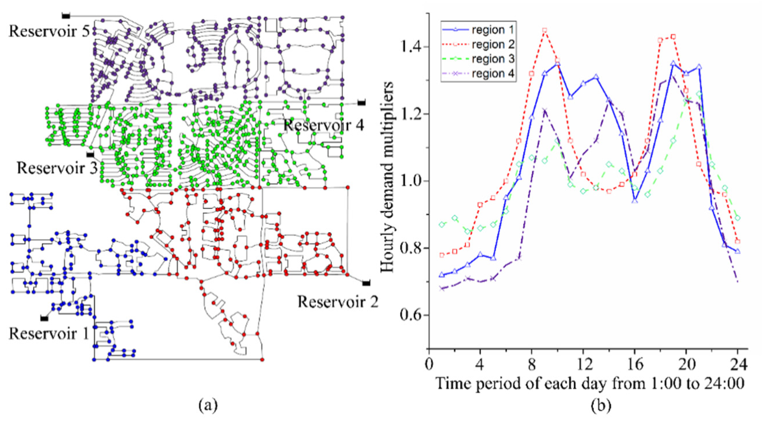
2.9. Water Distribution System Design Problems (WDSDP)

A realistic WDSDP (Figure 1a) with 935 demand nodes, 1278 pipes, 5 reservoirs and 24 demand loading cases [3] was used in this study to demonstrate the effectiveness of the proposed many-objective optimization framework for coping with complex systems. The WDS is divided into four regions according to the different water supply/demand patterns: 1 (blue), 2 (red), 3 (green) and 4 (purple), respectively. The hourly nodal demand multipliers for these four supply regions are shown in Figure 1b. As a result, the actual demand for each node is equal to the product of its nominal value and the pattern’s multiplier during that time period.

In this study, the minimum required and maximum allowable pressure for each node is set to 14 m and 60 m, respectively. For optimization, the diameter of each pipe is selected from a set of commercially available pipe diameters, as follows: (150, 200, 250, 300, 350, 400, 450, 500, 600, 700, 750, 800, 900, 1000) mm. EPANET 2.0 [24] was employed to compute the hydraulic conditions (nodal pressures and pipe flows) for each solution during the optimization process. The visual analysis tool, DiscoveryDV [9], was used to present and visualize the tradeoff relationships between different design objectives. It is highlighted that the visual analysis method was adopted from [2]. It is highlighted that flow velocity [25] is considered as the constraint in this study, where the minimum and maximum allowable flow velocity for each pipe is 0.3 m/s and 3 m/s, respectively, following [3].

3. Results and Discussion

Based on the developed many-objective optimization framework and the solution procedure, the results for the above-mentioned WDSDP are obtained to achieve the overall optimal situations of all the six objectives in the WDS system. The results and analysis are elaborated as follows.

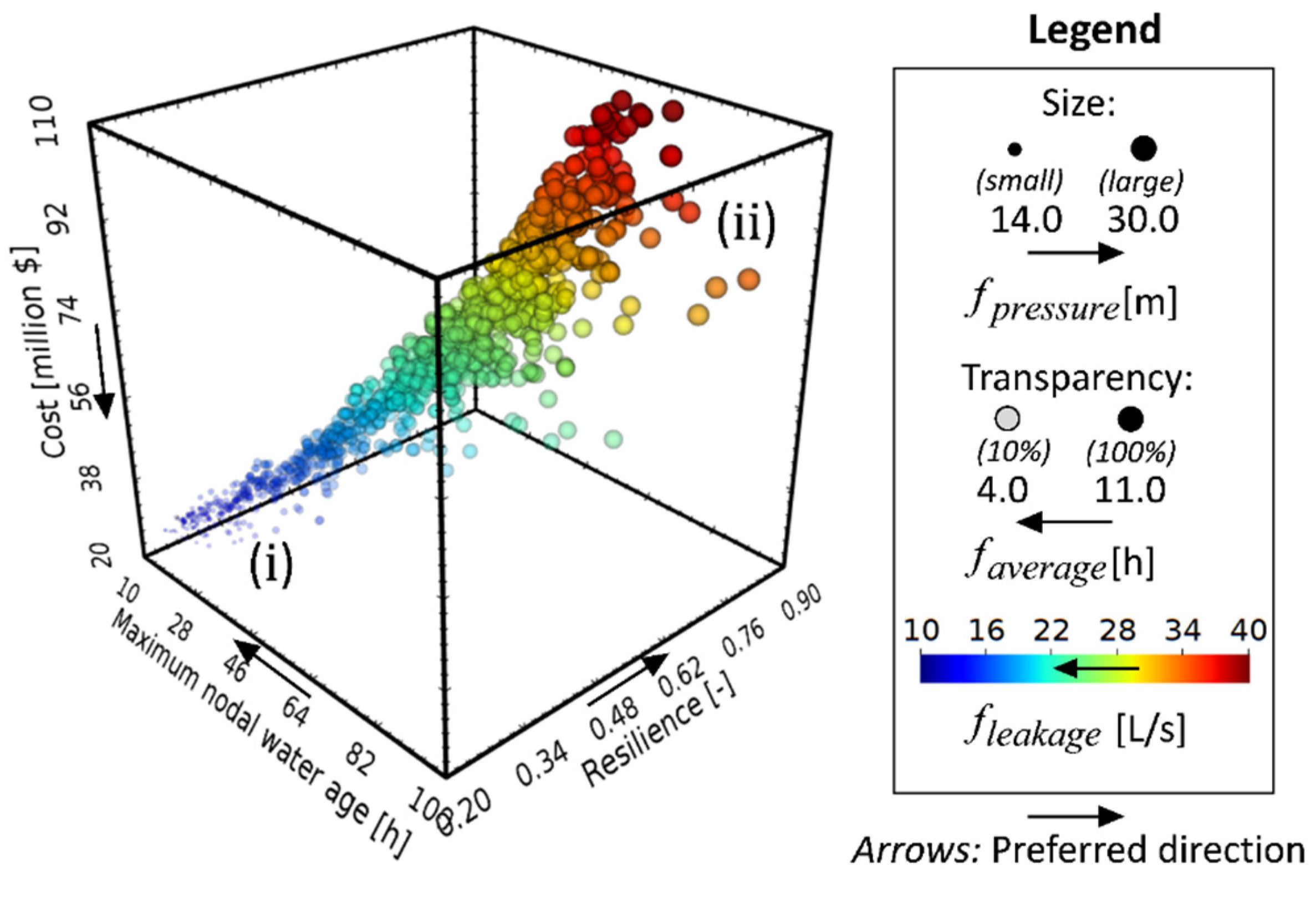
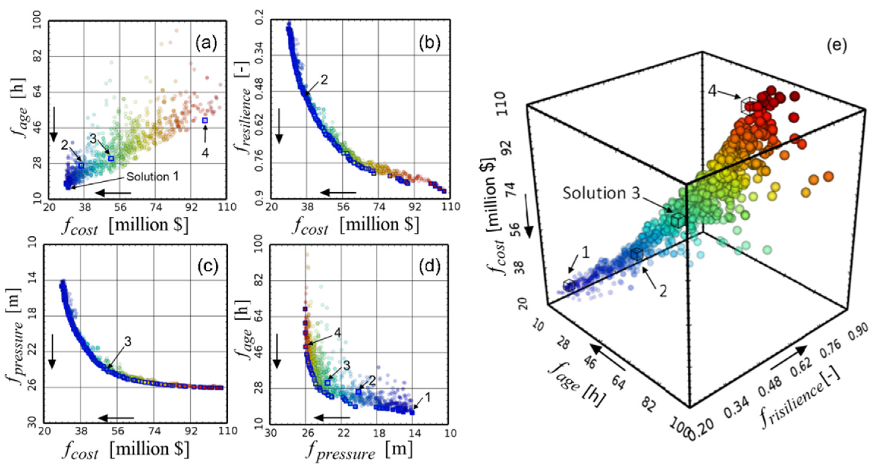
3.1. Exploring Tradeoffs in the Six-Objective Domain

A global view of the optimal results (Figure 2) is first analyzed to demonstrate the effectiveness of the many-objective optimization framework and method for the complex large-scale WDSDP, following the method described in [2]. Overall, the Pareto-optimal set for this design problem contains 1292 non-dominated solutions identified by the Borg method for all three independent runs, which took about 10 days on a computational platform with 3.00-GHz Intel Core i7-4710HQ with 16 GB of RAM. To visualize the optimized results of this six-objective problem, (1) the objectives of $f_{age}$, $f_{risilience}$ and $f_{cost}$ are plotted on the x-, y- and z-axis, respectively; (2) the objective $f_{pressure}$ is shown by the size of the spheres, in which the big spheres indicate high pressures and small spheres denote low pressures; (3) the objective of $f_{average}$ is represented by the transparency of the spheres with transparency ranging from 10% to 100%, representing the increasing average water age from 4.0 to 11.0 h; and (4) the $f_{leakage}$ objective is shown by the color of the spheres with colors ranging from blue to red, representing the increasing leakage from 10 to 40 L/s. Moreover, the black arrows in Figure 2 indicate the direction of preference for the specific objective (e.g., minimizing $f_{cost}$ and $f_{age}$, and maximizing $f_{risilience}$).

From the results of Figure 2, the region $\left(\mathrm{i}\right)$ is made up of solutions that have relatively small values in terms of cost (<$40 million), maximum water age at nodes (<20 h), average water age (<5.4 h) and leakage (<18 L/s), which trade off with relatively poor resilience (<0.4) and minimum nodal pressure (<20 m). That is, in this region (i), the obtained solutions may have smaller pipe diameters that result in lower costs, but would have larger velocity, lower water age and greater head loss from pipe roughness leading to lower pressure, leakage and resilience. On the contrary, the region $\left(\mathrm{ii}\right)$ in Figure 2 captures higher-preference solutions for achieving minimum nodal pressure and system resilience, trading off with relatively higher costs, maximum water age, average water age and leakage in the system. In other words, the design schemes obtained in this region may have larger pipe diameters that lead to higher surplus power compared with region ($\mathrm{i}$), which thus could improve the reliability (resilience) in handling water demand variations in the system.

A parallel line plot in Figure 3 is used to further analyze the correlations among these six different objectives, in which each solution is represented by a colored polyline with vertices on the parallel axes [9]. On one hand, the color of each parallel line varies in the range from blue to red, representing the increasing leakage from 10 to 40 L/s. On the other hand, the vertical position of each polyline in the figure represents the relative objective function value for each objective, with the arrow indicating the direction of preference for achieving that objective. For example, the blue polylines represent relatively low leakage solutions (e.g., within the region (i) in Figure 2), while the red polylines refer to relatively high leakage solutions (e.g., within the region (ii) in Figure 2). Furthermore, the parallel line plotting allows the geometrical features of a surface in a six-dimensional domain to be easily identified and therefore the relationships among different objectives can also be clearly visualized. For example, the crossing of different lines in Figure 3 implies the potential conflicts among these represented objectives during optimization process. Accordingly, the lines that do not cross indicate their corresponding objectives are in relative harmony with one another.

The two-objective subsets in the context of the full six-objective optimization domain provided in Figure 4 clearly show the correlations between any two objectives during the optimization process. In detail, Figure 4a–d shows the negative correlations of these tradeoff relationships between the different objectives. That is, any improvement in performance for one objective may result in potential degradation in performance for another objective. On the contrary, Figure 4e–h clearly reveals the positive correlations of these represented objectives during the optimization process.

It is also worth noting that the result of Figure 4g indicates a very weak correlation between the objectives of maximum water age and average water age used in this study. This is mainly because the average water age is a comprehensive indicator to assess water quality within the WDSs, which cannot directly indicate the time period from treatment plants to the nodes with the longest delivery time (maximum water age). For instance, when the average water age is 6 h (Figure 4g), the corresponding maximum water age range is 24 to 80 h, which thus results in conspicuous differences in these two water age objectives. On this point, the results have demonstrated the necessity of adopting the two objectives proposed in this study for a comprehensive optimization in WDSDP.

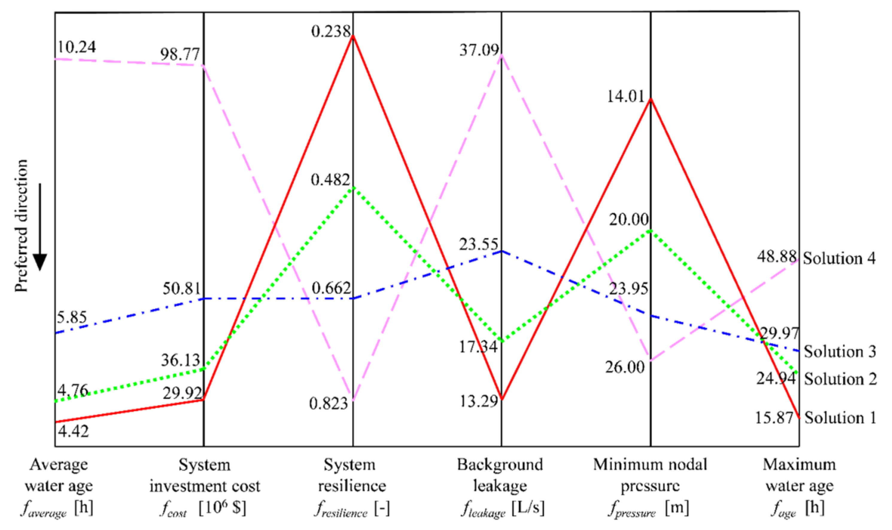
3.2. Selection Strategy of Optimal Design Scheme

With the results obtained from the many-objective optimization framework, it is important for the decision-makers to select the most suitable (“optimal”) design scheme for the specified WDS. The selection strategy for the optimal solution is illustrated herein through the above optimization results. For demonstration, four of the above various solutions have been selected according to their tradeoff relationships among conflicting objectives as shown in Figure 5a–d. The corresponding parallel lines for these selected objectives are shown in the supplemental data (Figure 6). One typical solution selection procedure that the stakeholders could take is illustrated as follows:

Figure 5a shows the tradeoff between the two objectives of $f_{cost}$ and $f_{age}$. Decision makers might first consider three aspects in the decision-making process: cost, water quality and leakage. In this way, solution 1, shown in Figure 5e, can then be identified to achieve the optimal performance for these three objectives.

Figure 5b shows the tradeoff between the two objectives of cost and resilience. In order to ensure higher network resilience in handling water demand variations, decision makers might choose solution 2, shown in Figure 5e, at the diminishing point of the cost–resilience tradeoff, so as to achieve higher resilience with a relatively lower cost.

Similar to the identification of solutions 1 and 2, solutions 3 and 4 can be found based on Figure 5c,d, respectively, in order to achieve a larger nodal pressure with a lower cost and a lower water age with a larger pressure. For clarity, the solutions are shown in Figure 5e.

Based on the results of the above solution selection strategy, their parallel lines plotted in Figure 6 clearly indicate the differences among the four solutions. Specifically, among these four solutions, solution 1 provides the best performance for average water age, cost, background leakage and maximum water age at nodes, but the worst performance for resilience and minimum pressure at nodes. However, solution 4 presents exactly the opposite trend of solution 1, leading to the best performance for resilience and minimum pressure at nodes, but the worst performance for the other objectives. Finally, solutions 2 and 3 provide better compromises among all the six objectives.

3.3. Further Discussion on the Solution Selection Results

Figure 7 shows the design results of the network layout for the four selected solutions. In particular, the results of the designed pipes for solutions 1 and 2 are in relatively small sizes, with diameters ranging from 200 to 500 mm and from 400 to 700 mm, respectively, while those for solutions 3 and 4 are largely above 700 mm, which are thus more expensive than solutions 1 and 2.

Figure 8 plots the underlying statistical distributions of the three hydraulic and water quality parameters—nodal pressure, water age and background leakage at each node for the four selected solutions. As observed in Figure 8a, the majority of the nodal pressure was between 15 m and 25 m for solution 1, between 20 m and 27 m for solution 2, between 24 m and 27 m for solution 3 and between 26 m and 27 m for solution 4. As a result, it is unsurprising that solution 1 has a relatively wider range of pressure distributions compared with the other solutions, and the range shrinks with the increase of pipe diameters (e.g., from solution 1 to solution 4). This is because the larger the pipe diameters, the smaller the head loss per unit length, and thus the smaller the pressure difference among different specified nodes. Figure 8b displays the probability distributions of the nodal water age for these selected solutions. The nodal water age distribution presents the exact opposite trend of nodal pressure distribution in Figure 8a. This is because the increase of pipe diameters may lead to a decrease of pipe velocity and therefore the increase of nodal water age. A similar relationship can be observed for the background leakage distribution in Figure 8c as with the water age, since the leakage objective is positively correlated with the water age objective during the optimization process as previously shown in Figure 2.

To further evaluate the solution’s reliability in handling water demand variations, Figure 9 plots the reliability differences of the four solutions in terms of nodal pressure, nodal water age and nodal background leakage under different demand loading conditions. A total of 50,000 demand loading samples were generated by the Monte Carlo random sampling method [1], and the results were used to calculate the probability density distributions of these three objectives for each selected solution under each demand loading condition. For each demand loading case, the actual demand of each node is randomly assigned within ±15% of its nominal demand value. As shown in Figure 9a, solution 1 presents the overall worst performance in handling water demand variations, while such imposed demand variations have little impact on the optimization objectives of the water age in Figure 9b and the background leakage in Figure 9c, respectively.

Consequently, the application results and analysis have demonstrated the feasibility and applicability of the developed many-objective optimization framework as well as the solution visualization method and selection strategy to complex and large-scale WDSDPs (with 6 objectives and 1278 decision variables).

4. Conclusions

This paper addresses the many-objective optimization problems of large-scale real-world WDS. A comprehensive framework is used to implement the six objectives commonly employed in WDS. The formulated optimization framework is then solved through the Borg-based MOEAs by visualizing and analyzing different objective tradeoffs for the decision-making process based on [2]. To demonstrate the effectiveness of the developed framework and methodology, a realistic large-scale WDSDP with 1278 decision variables and six objectives was applied in this study: the minimizations of (1) network cost, (2) average water age, (3) maximum water age at nodes, (4) leakage, and the maximizations of (5) minimum pressure at nodes and (6) network resilience. The strategy of design solution selection is also proposed through the case study.

The application results have shown that the framework was able to clearly reveal the important tradeoffs among these six different objectives, as well as significantly improve the understanding of the underlying characteristics of Pareto-front solutions with the aid of the interactive visualization approach for objective space analysis and decision space analysis [2]. The main findings of the present study include the following: (i) a weak correlation exists between the maximum water age and the average water age objectives, implying that the latter (typically used in the literature) is unable to represent the comprehensive water quality in the WDS; (ii) the proposed solution selection strategy from Pareto fronts (Section 3.2) is practically very meaningful as it can provide guidance for water managers to determine the most suitable WDS design solution; and (iii) the proposed method for evaluating the solution’s reliability in handling water demand variations (Figure 8) is effective in facilitating the selection of the appropriate solution, which has not been accomplished before to our best knowledge and hence represents an important contribution of this study. Overall, the proposed analysis method could be beneficial to many water managers and practitioners in selecting the most appropriate solution for a given WDS design problem. Future work should extend the proposed framework to deal with more complex WDSs with pumps, tanks and valves [26,27].

References

1. Huang, Y.; Duan, H.-F.; Zhao, M.; Zhang, Q.; Zhao, H.; Zhang, K. Probabilistic Analysis and Evaluation of Nodal Demand Effect on Transient Analysis in Urban Water Distribution Systems. J. Water Resour. Plan. Manag. 2017, 143, 04017041. [Google Scholar] [CrossRef]
2. Fu, G.; Kapelan, Z.; Kasprzyk, J.R.; Reed, P. Optimal design of water distribution systems using many-objective visual an-alytics. J. Water Resour. Plan. Manag. 2012, 139, 624–633. [Google Scholar] [CrossRef] [Green Version]
3. Zheng, F.; Zecchin, A.C.; Maier, H.R.; Simpson, A.R. Comparison of the Searching Behavior of NSGA-II, SAMODE, and Borg MOEAs Applied to Water Distribution System Design Problems. J. Water Resour. Plan. Manag. 2016, 142, 04016017. [Google Scholar] [CrossRef]
4. Wang, Q.; Guidolin, M.; Savic, D.; Kapelan, Z. Two-Objective Design of Benchmark Problems of a Water Distribution System via MOEAs: Towards the Best-Known Approximation of the True Pareto Front. J. Water Resour. Plan. Manag. 2015, 141, 04014060. [Google Scholar] [CrossRef] [Green Version]
5. He, G.; Zhang, T.; Zheng, F.; Zhang, Q. An efficient multi-objective optimization method for water quality sensor placement within water distribution systems considering contamination probability variations. Water Res. 2018, 143, 165–175. [Google Scholar] [CrossRef]
6. Qi, Z.; Zheng, F.; Guo, D.; Maier, H.R.; Zhang, T.; Yu, T.; Shao, Y. Better Understanding of the Capacity of Pressure Sensor Systems to Detect Pipe Burst within Water Distribution Networks. J. Water Resour. Plan. Manag. 2018, 144, 04018035. [Google Scholar] [CrossRef]
7. Qi, Z.; Zheng, F.; Guo, D.; Zhang, T.; Shao, Y.; Yu, T.; Zhang, K.; Maier, H.R. A Comprehensive Framework to Evaluate Hydraulic and Water Quality Impacts of Pipe Breaks on Water Distribution Systems. Water Resour. Res. 2018, 54, 8174–8195. [Google Scholar] [CrossRef]
8. Zhang, Q.; Zheng, F.; Duan, H.-F.; Jia, Y.; Zhang, T.; Guo, X. Efficient Numerical Approach for Simultaneous Calibration of Pipe Roughness Coefficients and Nodal Demands for Water Distribution Systems. J. Water Resour. Plan. Manag. 2018, 144, 04018063. [Google Scholar] [CrossRef]
9. Kollat, J.B.; Reed, P. A framework for Visually Interactive Decision-making and Design using Evolutionary Multi-objective Optimization (VIDEO). Environ. Model. Softw. 2007, 22, 1691–1704. [Google Scholar] [CrossRef]
10. Pietrucha-Urbanik, K. Assessment Model Application of Water Supply System Management in Crisis Situations. Glob. Nest J. 2014, 16, 893–900. [Google Scholar]
11. Pietrucha-Urbanik, K.; Studziński, A. Qualitative analysis of the failure risk of water pipes in terms of water supply safety. Eng. Fail. Anal. 2019, 95, 371–378. [Google Scholar] [CrossRef]
12. Geem, Z.W.; Kim, J.H.; Loganathan, G.V. A new heuristic optimization algorithm: Harmony search. Simulation 2001, 76, 60–68. [Google Scholar] [CrossRef]
13. Simpson, A.R.; Dandy, G.C.; Murphy, L.J. Genetic Algorithms Compared to Other Techniques for Pipe Optimization. J. Water Resour. Plan. Manag. 1994, 120, 423–443. [Google Scholar] [CrossRef] [Green Version]
14. Cunha, M.D.C.; Sousa, J. Hydraulic Infrastructures Design Using Simulated Annealing. J. Infrastruct. Syst. 2001, 7, 32–39. [Google Scholar] [CrossRef]
15. Maier, H.; Simpson, A.R.; Zecchin, A.C.; Foong, W.K.; Phang, K.Y.; Seah, H.Y.; Tan, C.L. Ant Colony Optimization for Design of Water Distribution Systems. J. Water Resour. Plan. Manag. 2003, 129, 200–209. [Google Scholar] [CrossRef] [Green Version]
16. Cunha, M.; Marques, J. A New Multiobjective Simulated Annealing Algorithm—MOSA-GR: Application to the Optimal Design of Water Distribution Networks. Water Resour. Res. 2020, 56, e2019WR025852. [Google Scholar] [CrossRef]
17. Fu, G.; Butler, D.; Khu, S.-T. Multiple objective optimal control of integrated urban wastewater systems. Environ. Model. Softw. 2008, 23, 225–234. [Google Scholar] [CrossRef]
18. McInnis, D.; Karney, B.W. Transients in Distribution Networks: Field Tests and Demand Models. J. Hydraul. Eng. 1995, 121, 218–231. [Google Scholar] [CrossRef] [Green Version]
19. Marsili, V.; Meniconi, S.; Alvisi, S.; Brunone, B.; Franchini, M. Stochastic Approach for the Analysis of Demand Induced Transients in Real Water Distribution Systems. J. Water Resour. Plan. Manag. 2022, 141, 04021093. [Google Scholar] [CrossRef]
20. Huang, Y.; Zheng, F.; Duan, H.-F.; Zhang, Q. Multi-Objective Optimal Design of Water Distribution Networks Accounting for Transient Impacts. Water Resour. Manag. 2020, 34, 1517–1534. [Google Scholar] [CrossRef]
21. Prasad, T.D.; Park, N.-S. Multiobjective Genetic Algorithms for Design of Water Distribution Networks. J. Water Resour. Plan. Manag. 2004, 130, 73–82. [Google Scholar] [CrossRef]
22. Hadka, D.; Reed, P. Borg: An Auto-Adaptive Many-Objective Evolutionary Computing Framework. Evol. Comput. 2013, 21, 231–259. [Google Scholar] [CrossRef]
23. Reed, P.M.; Kollat, J.B. Visual analytics clarify the scalability and effectiveness of massively parallel many-objective optimi-zation: A groundwater monitoring design example. Adv. Water Resour. 2013, 56, 1–13. [Google Scholar] [CrossRef] [Green Version]
24. Rossman, L.A. EPANET 2: Users Manual; National Risk Management Research Laboratory: Cincinnati, OH, USA, 2000. [Google Scholar]
25. Geem, Z.W. Multiobjective Optimization of Water Distribution Networks Using Fuzzy Theory and Harmony Search. Water 2005, 7, 3613–3625. [Google Scholar] [CrossRef]
26. Zheng, F.; Simpson, A.R.; Zecchin, A. A combined NLP-differential evolution algorithm approach for the optimization of looped water distribution systems. Water Resour. Res. 2011, 47, 2924–2930. [Google Scholar] [CrossRef] [Green Version]
27. Zheng, F.; Zecchin, A.; Newman, J.P.; Maier, H.; Dandy, G.C. An Adaptive Convergence-Trajectory Controlled Ant Colony Optimization Algorithm with Application to Water Distribution System Design Problems. IEEE Trans. Evol. Comput. 2017, 21, 773–791. [Google Scholar] [CrossRef]
Figure 1. (a) The layout of the studied WDS, with the blue, red, green and purple nodes representing supply regions 1, 2, 3 and 4 for different nodal demand patterns, respectively. (b) The hourly demand multipliers for supply regions 1, 2, 3 and 4.
Water 14 00557 g001
Figure 2. Global view of the six-objective Pareto-optimal solution set, with arrows pointing in the direction of preference.
Water 14 00557 g002
Figure 3. Parallel line plot for the Pareto approximate set (each colored polyline with vertices on the parallel axes represents the objective vector for a single solution, with the arrow pointing in the direction of preference).
Water 14 00557 g003
Figure 4. Selected two-objective subsets in the context of the full six-objective space: (a) fcost versus fresilience; (b) fage versus fresilience; (c) fage versus fpressure; (d) fcost versus fpressure; (e) fpressure versus fresilience; (f) fcost versus faverage; (g) fage versus fresilience; and (h) fage versus fcost.
Water 14 00557 g004
Figure 5. Four representative solutions identified based on a two-dimensional tradeoff: (a) fage versus fcost; (b) fcost versus fresilience; (c) fcost versus fpressure; (d) fage versus fpressure, and (e) global view.
Water 14 00557 g005
Figure 6. Parallel line plot for the four solutions (vertices of each line on the parallel axes representing the objective function values for a single solution, with arrows pointing in the direction of preference and the red, green, blue and purple lines represent solution 1, solution 2, solution 3 and solution 4, respectively).
Water 14 00557 g006
Figure 7. Design results of pipe diameters for the four selected solutions: (a) solution 1, (b) solution 2, (c) solution 3, and (d) solution 4.
Water 14 00557 g007
Figure 8. Probability density distributions of the three key indicators for the four solutions: (a) nodal pressure, (b) water age, and (c) background leakage. (The red, green, blue and purple lines represent solution 1, solution 2, solution 3 and solution 4, respectively).
Water 14 00557 g008
Figure 9. Probability density distributions of the three key indicators for the four solutions under 50,000 demand loading cases: (a) nodal pressure, (b) water age and (c) background leakage.
Water 14 00557 g009
Publisher’s Note: MDPI stays neutral with regard to jurisdictional claims in published maps and institutional affiliations.