1. Introduction
Typical flood defense infrastructure design is tackled as a sequential application of deterministic formulas and models, fed by a hypothetical storm event (hyetograph) that follows a prespecified temporal pattern (e.g., alternating blocks) and corresponds to a desirable return period [
1]. In this procedure, the unique probabilistic concept is that of the return period of the design rainfall, which is set a priori, to denote the acceptable probability of exceedance of all quantities of interest associated with flood hazard assessment (peak flows, flood hydrographs, flow depths and velocities, inundated areas, etc.).
Arguably, this so-called event-based approach is considered particularly risky in the context of hydrological infrastructure design [
2], due to the oversimplification, ignorance, or misuse of important concepts and mechanisms of the rainfall–runoff transformation. Specifically:
The role of varying and, thus, uncertain antecedent soil moisture conditions, which are a major driver of floods, is ignored [
3,
4].
The simplified and deterministically specified shape of input hyetographs, as well as the concept of critical rainfall duration [
5], is far from representative of the actual probabilistic regime of extreme storm events [
6,
7].
The time parameters that are embedded in the description of routing processes (time of concentration, lag time, etc.) are handled as constant properties rather than flow-dependent variables [
8,
9].
The spatial heterogeneity of storms is not included in the analysis, although this can be a rather important factor, especially in rainfall events generated by orographic phenomena [
10,
11].
The probability (or, equivalently, return period) of rainfall is considered as a proxy of the flood probability [
12]—a key hypothesis that is yet strongly influenced by the rainfall mechanisms and the catchment characteristics [
13].
To address the above challenges, as well as the multiple complexities and uncertainties that span over the whole spectrum of the flood generation, routing, and drainage processes (also affected by the changing climate), the hydrological community has called for more integrated approaches in flood modeling, which follow the continuous simulation concept [
14,
15,
16]. The generic definition of simulation refers to the representation of a dynamic (i.e., changing) system in the long run, preferably using synthetic data that are statistically equivalent to the observed ones (thus, the correct term should be
continuous stochastic simulation). In the context of a drainage system (e.g., a river basin), this approach allows for investigating its response (e.g., the generation of flood runoff) against a wide range of inputs (i.e., rainfall events) and states (i.e., soil conditions), with different probabilities.
The major shortcoming of continuous stochastic simulation over event-based deterministic approaches is the substantially larger computational effort. This is induced by the need for running time-demanding process representation models, namely, rainfall–runoff and hydraulic (better referred to as hydrodynamic), with finely resolved data, induced by the typically small temporal scale of interest (e.g., 15-min), which extend over very long horizons. For instance, in order to evaluate probabilistic quantities that correspond to a
T-year return period through empirically based statistical approaches (e.g., Monte Carlo analysis), the underlying sample size should be much larger [
17]. Furthermore, the rainfall–runoff and hydrodynamic models should be fully coupled to allow for representing the flood generation and routing processes with satisfactory accuracy, thus making the whole approach extremely difficult, if not prohibitive, for the engineering community and practicians [
18]. For this reason, continuous simulation and stochastic event-based methods are often tackled as alternative approaches [
19]. Other alternatives are based on “semi-continuous” schemes, where synthetic rainfall events are inserted into continuous historical rainfall records, and then used in hydrological models [
20].
In order to handle the flood hazard assessment challenge by ensuring an acceptable compromise between realism and consistency in process representation, as well as computational effectiveness and feasibility, we propose a hybrid framework, which is implemented through a cascade of stochastic, rainfall–runoff, and hydrodynamic simulation models of different levels of detail (1D and coupled 1D/2D). The overall approach is founded on the Monte Carlo paradigm, by retaining the fundamental concept of return period of the design rainfall at the 24 h scale. In this vein, for specific return periods, the flood hazard and resulting risk (i.e., combination of hazard and adverse consequences) are evaluated through a wide range of synthetically generated scenarios of potential states (i.e., soil moisture conditions) and inputs (i.e., rainfall patterns) with different probabilities. This allows assessing the system’s performance when pushed outside the deterministic (regulation-based) design events, a procedure which is becoming known as “resilience assessment” [
21]. The methodology is demonstrated in a real-world hydraulic design study, involving an urban stream in the southwestern Attica region, Greece (Trachones stream and its main drainage network), which crosses highly urbanized suburbs of the Athens Metropolitan area, while also including lands of exceptional commercial value in its downstream region.
2. The Hybrid Stochastic Simulation Framework in a Nutshell
The concept of flood hazard and, eventually, flood risk, under the prism of stochastic simulation, entails the modeling of all important processes across the drainage system, their forcing through stochastically generated drivers, and the subsequent statistical description of the resulting effects in the areas of interest. Ideally, this should be a continuous procedure, to enable a direct statistical analysis of the simulated flooding data. However, as already highlighted, in the context of common engineering practice, such simulations are still computationally infeasible. Therefore, another approach must be considered, to ensure a reasonable balance between accuracy in the representation of uncertainties and the computational cost. In this context, it is useful to conceptualize the stochastic simulation procedure as a chain of cascading modules, i.e., weather generation (through a timeseries synthesis model), rainfall–runoff transformation (through a hydrological model), and hydraulic routing (through a hydrodynamic model).
In this vein, the key uncertainties of each module are explicitly handled and next transferred to subsequent modules by means of input–output exchanges. As shown in
Table 1, the proposed framework pays attention to statistical and process uncertainties, while other sources of uncertainty (structural, parametric) are ignored, e.g., those associated with the hydraulic modeling (e.g., roughness conditions, model of choice, survey and topographic data accuracy, and structure attributes) [
22].
Having established the main uncertainties, we can now introduce the overall simulation approach, involving the sequential application of different modeling tools and associated data exchanges, as illustrated in
Figure 1. A more detailed description of individual models and their key novelties is made in the subsequent sections.
Firstly, synthetic rainfall on the daily scale is generated for years, where has to be large enough to provide statistically reliable estimations of extreme probabilistic quantities. The daily scale is proposed in order to avoid the large computational cost associated with generating long synthetic timeseries for sub-daily scales. Then, a statistical model for the extreme annual rainfall is fitted to the synthetic data, on the basis of which values are inferred for return levels of interest. Next, sub-daily storm events are generated by disaggregating the associated daily rainfall values at the desired fine scale of hydrological and hydrodynamic simulation (in our case, 15 min). This procedure simultaneously addresses the main uncertainties associated with the stochastic simulation of the extreme rainfall, while also retaining a low computational cost.
Subsequently, the catchment state (i.e., soil moisture conditions) is associated with the antecedent cumulative rainfall (here referred to the 60 day scale, as result of the dry regime of the study area) and mapped to the key, spatially distributed input of the rainfall–runoff modeling procedure, i.e., the curve number, . The stochastic storm events and the randomly generated system states (in terms of values) become inputs to a semi-distributed event-based hydrological model, i.e., the NRCS-CN. The time-related inputs of the system (i.e., unit hydrograph and channel velocities) are also allowed to vary, according to the severity of the storm event. In this manner, the two main uncertainties regarding the rainfall–runoff processes are treated, whereas the effective rainfall generation mechanism is a priori assumed.
The outputs of hydrological simulations, i.e., the flood hydrographs, are assigned as point inflows (inflow boundary conditions) to a hydrodynamic simulation model of the drainage network (stream/river) in the lower course of the catchment, which is our area of interest. In order to address the computational cost associated with detailed simulation (e.g., 2D) we propose a hybrid 1D/2D scheme. Specifically, we first employ the 1D model to run the entire set of storms. On the basis of the results, the so-called critical scenarios are identified and subsequently simulated in the detailed model. These are defined on the basis of a priori determined thresholds that are exceeded by the variables of interest (e.g., flow velocity, water level etc.). As a result, the detailed simulations produce scenarios of flood extents that are statistically analyzed to obtain the relevant flood hazard metrics, while the 1D simulations produce useful statistics across all simulated flood events.
In the next sections, the individual components of the framework are discussed in detail according to the specific case study presented herein. While in the implementation of the proposed framework, specific tools are employed and some of their inputs and assumptions are by definition based on local data, the framework is—by construction—nonexclusive. In contrast, it allows for the integration of any models/tools which are capable of addressing the associated uncertainties and producing the required results.
3. Study Area and Data
Trachones is an urban stream that drains an area of 23.48 km2, which extends in the south Athenian plain, between the foothills of Mount Hymettus and the southern coastal zone of Athens (Saronikos Gulf). Its drainage network, which mainly crosses urbanized areas, is formulated by two main branches and several smaller tributaries. The lower course of the stream lies in the northern boundary of the so-called Metropolitan Pole of Hellinikon–Agios Kosmas, which is a planned urban development on the site of the former International Airport of Athens, covering an area of approximately 6.2 km2. The exceptional character of this investment makes the proper assessment of flood hazard across these areas even more challenging.
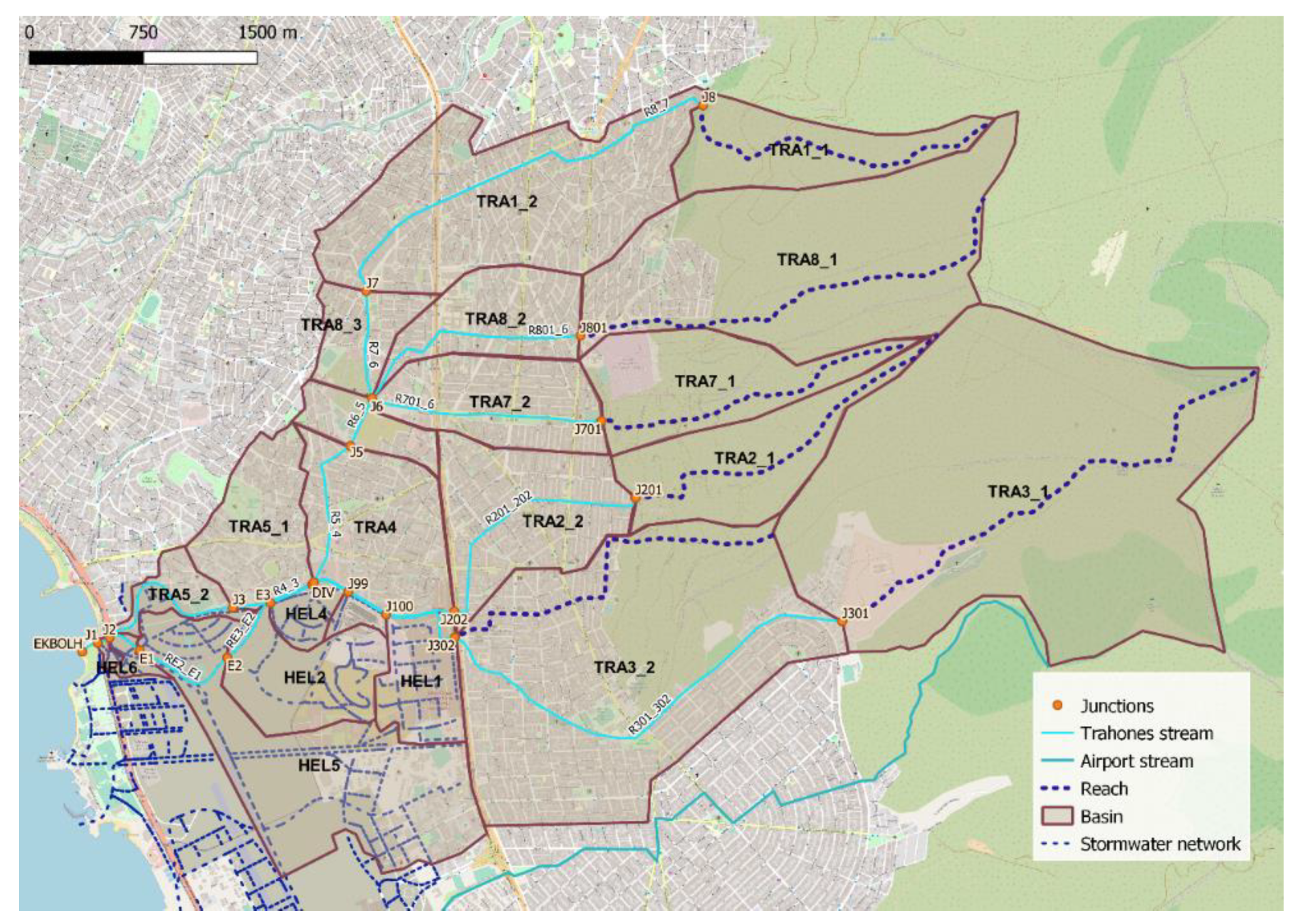
In the context of hydrological analyses, the flood generation and routing processes are represented through a conceptual semi-distributed scheme, which is implemented in the HEC-HMS environment. As shown in
Figure 2, the drainage area is divided into 22 sub-basins, while the flood flows are conveyed through a reach network comprising 20 elements, including natural channels (mainly in the upstream parts) and storm sewers (open channels, closed conduits). The level of detail of this schematization is dictated by the corresponding level of analysis of the underlying design study. Given that only limited parts of the downstream network are still open, in order to delineate the sub-basin boundaries within the urban environment and identify the actual water paths across the covered parts of the natural stream network, we took advantage of topographic maps from the late 19th century and macroscopic information retrieved from satellite maps.
Since the catchment is ungauged, the sole hydrometeorological information used in this study was a daily rainfall record, retrieved from the Hellinikon meteorological station. The raw data were logged in 12 h intervals and cover a period of 65 years (from 1955 to 2019), without gaps. Due to the relatively small extent of the study area, we considered this station as representative of the rainfall regime of the overall catchment.
4. Weather Generation
To incorporate the meteorological uncertainty within flood hazard assessment, rainfall is treated as a stochastic process, through the use of probabilistic methods and stochastic simulation techniques. This approach enables the generation of a large number of synthetic rainfall timeseries, by means of storm events (hyetographs) of 15 min resolution, which are statistically consistent with the historical data. These are then used as inputs to deterministic simulation models, allowing an analysis of their response under uncertainty.
In this research, two main aspects of uncertainty are examined and modeled. The first concerns the statistical uncertainty associated with the estimation of 24 h annual rainfall maxima, which is, by definition, impossible to be completely eliminated, due to the finite length of historical data, as well as the sampling uncertainties and/or biases. The second aspect regards the temporal distribution of rainfall events (i.e., storm profile), which plays a key role in the generation of floods; recall that a given rainfall total (e.g., 24-h event) can be the aggregated outcome of an infinite number of lower-temporal-level rainfall events (in the specific case, hyetographs of 15 min resolution).
Aiming to address the first aspect mentioned above, we use the
anySim R-package that allows the simulation of realizations of stochastic processes with any marginal distribution and autocorrelation structure [
23]. Through this tool, we generate 10,000 years of synthetic daily rainfall by employing the multitemporal simulation module of the package that couples two stochastic models, one for the annual scale and one for the daily one [
24]. Taking advantage of the daily data, we further analyze the probabilistic behavior of daily annual maxima. Specifically, we first extract from the full synthetic sample the subset of daily annual maxima (10,000 values); next, we obtain estimates for both the distribution of daily (more precisely, 24-h) maxima, as well as its confidence levels,
. In this respect, we apply a procedure that combines the generalized extreme value (GEV) distribution with a Monte Carlo resampling fitting approach [
25], to provide estimations for 10 characteristic return periods,
(years) and for
. The results are depicted in
Figure 3. For instance, for
years and
, the daily rainfall intensity is 5.89 mm/h (this value corresponds to a daily depth of 141.4 mm); it is noted that the maximum value of daily rainfall intensity of the historical sample (subset of 62 daily annual maxima) is 5.91 mm/h.
Next, we generate (also using
anySim) a number of synthetic rainfall hyetographs, at the timescale of interest, i.e., 15 min, which correspond to the desirable return periods and confidence levels of the daily maximum rainfall. This implies that the cumulative rainfall of each hyetograph, consisting of 96 partial depths, should equal the 24 h rainfall value, dictated by the corresponding combination of
and
. This challenging task is employed through (a) a novel downscaling approach for reconstructing the key statistical properties (i.e., mean, variance, probability dry, and autocorrelation) at the timescale of interest [
26], (b) a multiscale distribution fitting approach, using the Burr type XII distribution [
27], and (c) a novel, recently introduced disaggregation approach [
26] to disaggregate the 24 h maximum rainfall values to the temporal level of 15 min. We underline that the first two steps are required due to the lack of raw data at the required resolution. If such data were available, only step (c) would be necessary, as the key statistical quantities at that timescale would be inferred from the historical sample.
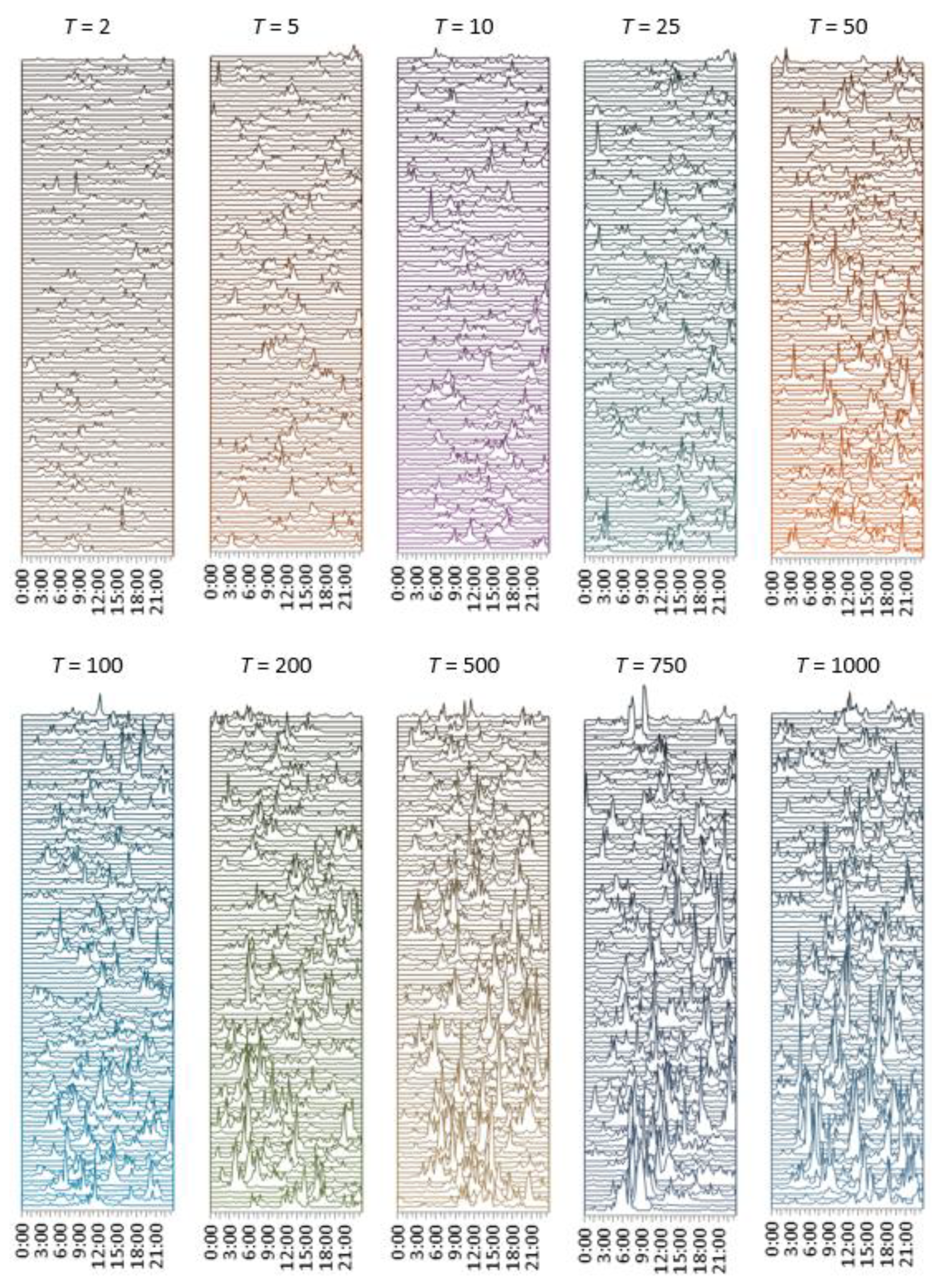
We remark that, for each return period
(10 in total) and confidence level
(five in total), we generate 20 equally probable hyetograph realizations, aiming to account for the uncertainty in the time profile of rainfall at the temporal resolution of 15 min. Overall, the total number of storm events (i.e., hyetographs) is
, preserving the desirable marginal distribution and autocorrelation structure, as well as summing up to the parent 24 h rainfall. The
synthetic hyetographs, grouped per return period
, are depicted in
Figure 4.
5. Rainfall–Runoff Modeling
5.1. Overview
The flood simulation procedure implements the semi-distributed schematization of the Trachones system, comprising 22 sub-basins and 20 reach elements, through the HEC-HMS package. At the sub-basin level, the model estimates the generation of surface runoff over the drainage area (effective rainfall), by employing a modified version of the NRCS-CN method, where its key input, i.e., the runoff curve number, , is handled as a stochastic variable. Eventually, the model is driven with the 1000 synthetically generated storm events, while, for each rainfall scenario, a random value of CN is assigned, in order to account for the variability of antecedent soil moisture conditions at the beginning of each storm event. As explained next, these are expressed in terms of 60 day accumulated rainfall, and then mapped to .
The effective rainfall produced over each sub-basin is next routed to the corresponding outlet junction, through the unit hydrograph method. The key assumption here is the dynamic change of the hydrograph shape against the varying rainfall, as a result of the dependence of the response time of the basin on the flow conditions.
The hydrographs arriving at all junctions are eventually propagated through the reach network, by applying routing schemes (lag time, for steep slopes, and Muskingum method, for mild ones). The time parameter of both methods is also adapted to the changing flow conditions of each simulated event, via an original velocity approach.
5.2. The NRCS-CN Method in Stochastic Pseudo-Continuous Setting
5.2.1. The Standard NRCS-CN Method
The NRCS-CN method, introduced by the Soil Conservation Service in 1954 (today referred to as the Natural Resources Conservation Service, NRCS), is recognized as the most widely used event-based scheme globally. This method describes the temporal evolution of surface (flood) runoff (also referred to as effective rainfall,
) from a given cumulative rainfall,
h, through the following empirical formula [
28]:
where
and
S are two lumped parameters over the drainage area of interest (in our case, sub-basin), namely, the initial deficit and the maximum potential retention; the latter is typically defined as
(all values are expressed in mm). Furthermore, it maps
S into a dimensional quantity, referred to as runoff curve number,
, i.e.,
is a conceptual metric, ranging from 1 to 100, which captures, in a unique value, the major physiographic properties that are associated with runoff generation over an area of interest. According to the SCS/NRCS standards, this depends on soil and land-cover characteristics, as well as on the moisture present in the soil profile before a rainfall event. The literature provides
values for average soil moisture conditions and the typically used initial abstraction ratio
(herein referred to as reference conditions). The recommended values are expressed by means of lookup tables, accounting for several combinations of land-use/land-cover characteristics and four hydrological soil types [
28].
5.2.2. On the Representativeness of 5 Day Accumulated Rainfall for Classifying AMC Types
The standard NRCS-CN approach considers three discrete antecedent soil moisture conditions (AMC I, II and III), depending on the total 5 day antecedent rainfall and the season category (dormant or growing). The so-called dry, average, or wet soil states have been derived through field experiments, mainly employed in small agricultural catchments in USA. In the literature, the determination of AMC, which is an index of the basin wetness, has been subject to major critique, due to the limited information about its definition [
29]. Nevertheless, it is accepted that the
values associated with AMC-II represent a central tendency, while those associated with AMC-I and AMC-III are representative of extremes of the runoff frequency distribution [
30].
For convenience, the reference
is determined for average conditions (AMC II), while, for the other two AMC types, NRCS provides the following empirical conversion formulas [
28]:
Although the 5 day cumulative rainfall is the typical indicator of the actual soil moisture conditions within the NRCS-CN scheme, it is also questionable whether this quantity is representative across all hydroclimates [
31]. In particular, in arid, semiarid, and dry areas (which is our case), characterized by intense yet not often storm events, and long periods with minimal and even zero rainfall, the definition of AMC on the basis of 5 day rainfall may lead to far from plausible outcomes. Therefore, an essential question to address is the aggregation scale of rainfall ensuring a reasonable determination of antecedent soil moisture conditions.
In this respect, and following the rationale by Hjelmfelt [
30], it is assumed that the classification of dry, normal, and wet soil moisture conditions (and, consequently, the adjustment of reference
values according to Equation (3)) corresponds to 10%, 50%, and 90% probability of non-exceedance of the
n-day cumulative rainfall, where
n denotes the scale of aggregation. Using the daily rainfall record from the Hellinikon meteorological station from 1955 to 2019, we calculate the cumulative rainfall for four aggregation levels (
n = 5, 15, 30, and 60 days), and estimate the three characteristic quantiles, as well as three more extreme ones (1%, 99%, and 99.9%). The results are summarized in
Table 2. It is remarkable that for all scales except for the 60 day one, the aggregated rainfall assigned to dry conditions (10% quantile) is zero, while, for the 60 day scale, this value is only 1.9 mm. In this respect, we consider the characteristic values of 60 day rainfall,
, as thresholds for recognizing the discrete soil conditions introduced by NRCS (dry, normal, wet), as well as the very dry, very wet, and extremely wet states.
5.2.3. Mapping of Curve Number to Antecedent Soil Moisture Conditions
Several researchers have revealed the limitations of the NRCS-CN method with respect to soil processes and proposed further parameterization to better represent the initial soil moisture conditions [
3,
5,
32]. Today, there are numerus continuous simulation variants of the original event-based scheme that allow explicitly representing the variability of rainfall and antecedent soil moisture conditions, mainly via soil moisture accounting procedures [
33,
34,
35,
36].
Instead of a soil moisture accounting scheme, the proposed approach employs a continuous classification of antecedent soil moisture conditions, by mapping the reference
across sub-basins to the 60 day accumulated rainfall (hereafter symbolized
), which is by definition a stochastic process. In particular, initially, we apply Equation (3) to obtain the adjusted values for dry and wet AMCs. Under the premise that
,
, and
correspond to non-exceedance probabilities
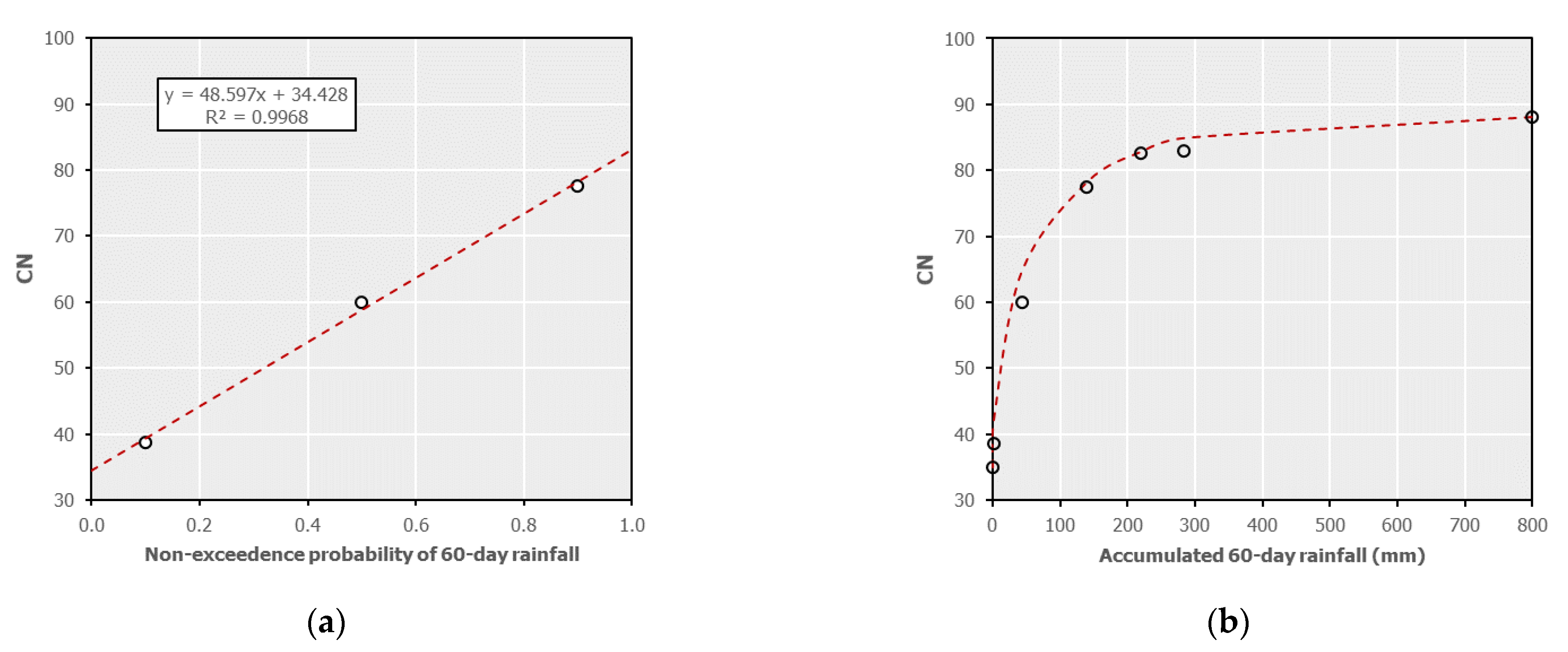
p = 0.50, 0.10, and 0.90, respectively, we establish the following probabilistic expression:
where
denotes a theoretically lowest value of the curve number under extremely dry conditions (
,
is a rate parameter, and
is the non-exceedance probability of 60 day rainfall. The two unknown quantities,
and
, are empirically determined through regression, as shown in the example of
Figure 5a. The variation of
against antecedent soil moisture conditions, as expressed in terms of the probabilistic term
, indicates an asymptotic behavior of the curve number parameter with respect to past rainfall, which has also been confirmed by several researchers [
37]. In this vein, for each reference
, a theoretically upper value,
, needs to be assigned, driven by a hypothetically maximum potential antecedent 60 day rainfall,
, that corresponds to fully saturated soil conditions and whose non-exceedance probability tends to one (
). After preliminary investigations, we set
mm, which is about two times the mean annual rainfall at Hellinikon station (357.9 mm) and over the broader Athenian region, in general.
The nonlinear dependence of
against
through Equation (5) is well approximated by the following formula:
where
and
are the curve number and accumulated rainfall for very dry conditions,
and
are referred to as the asymptotic curve number and asymptotic accumulated rainfall, respectively, and
and
are shape parameters.
is manually set to 800 mm, thus indicating an accumulated 60 day rainfall value with negligible probability of exceedance,
is estimated by applying Equation (4) for each specific reference curve number, and
is also manually adjusted to
. The two shape parameters are empirically derived as
and
, by fitting Equation (5) to a sample of data generated for various reference values of
and associated probabilities. A graphical demonstration of the adjusting procedure, for reference
, is shown in
Figure 5b.
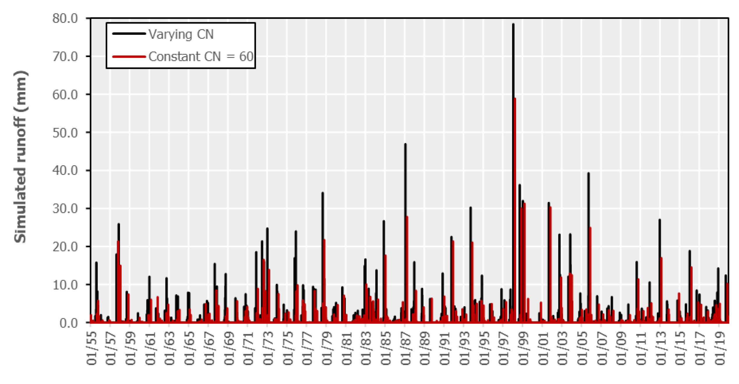
In the absence of observed data, and in order to evaluate our approach at least from an expert’s judgment perspective, we employ a hypothetical lumped configuration of the NRCS-CN method in fully continuous mode, for alternative
values (60, 70, 75, and 80). The model is driven with the observed daily rainfall data at Hellinikon station, as well as the 60 day aggregated rainfall data, which is representative of the antecedent soil moisture conditions. The flood runoff is extracted on a daily basis through Equation (1), where the maximum potential retention,
S, is estimated by mapping
to the 60 day rainfall, through the generalized formula in Equation (5). In
Figure 6, we contrast the simulated daily runoff by the standard NRCS-CN approach with
, and by the modified model with varying
around the same reference value. As expected, the second approach ensures a larger fluctuation of runoff, which is induced by the variability of antecedent soil moisture conditions, as reflected in the accumulated 60 day rainfall before each event. Apparently, it also provides larger peaks, which are associated with wet soil conditions, thus resulting in a quite larger average runoff, i.e., 35.0 mm on a mean annual basis, in contrast to the conventional approach that generates only 18.6 mm (as already mentioned, the mean annual rainfall is 357.9 mm). From our experience, the first value is more reasonable, since it ensures an average runoff coefficient close to 10%, which is consistent with the hydroclimatic regime of the broader area of Attica. In
Table 3, we also provide a comparison of the two datasets, in terms of marginal statistics of non-zero data.
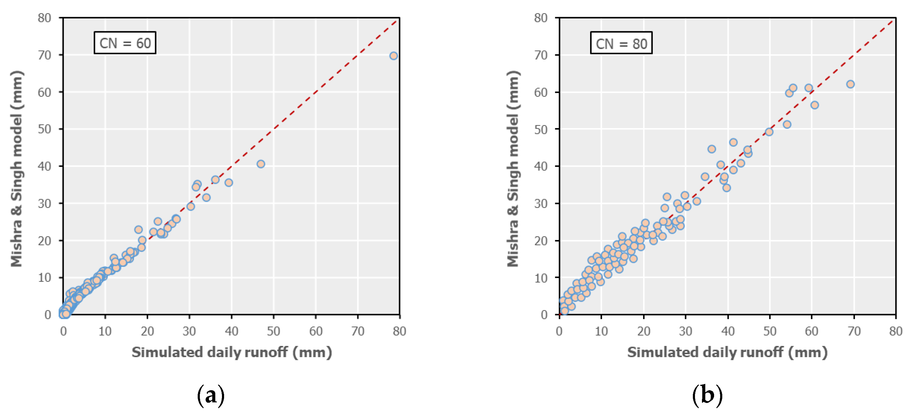
For further justification, the results are also compared with the simulated data obtained by the continuous simulation scheme by Mishra and Singh [
38]. In order to ensure consistency, the above model is also applied by considering the 60 day accumulated rainfall in the estimation of moisture component, and by setting λ = 0.05 for the estimation of initial abstraction losses. As shown in
Figure 7, the two methods provide close estimations of daily flood runoff, while our approach is considered more realistic, given that the variability of
is adjusted to the local rainfall regime, through the probabilistic Equation (4).
5.2.4. Pseudo-Continuous Implementation of NRCS-CN Method in the Study Area
While the proposed variation of the NRCS-CN method is fully compatible with the continuous simulation paradigm, its direct implementation would be computationally inefficient (as the underlying model is driven with synthetic data) and, eventually, nonessential, since our focus is on extreme storm events. In this respect, we employ a pseudo-continuous (i.e., scenario-based) procedure, where, for each of the 10 return periods of interest, with correspondence to the 24 h rainfall, the model receives 5 × 20 = 100 (i.e., 20 realizations for five ) equally probable scenarios of storm profiles and spatially distributed values over the sub-basins. To calculate the latter, we generate 1000 (10 × 100) random rainfall values, from the distribution of 60 day accumulated rainfall. Next, for each sub-basin, using as a guide the reference , we utilize Equation (5), thus running the NRCS-CN method with 1000 randomly generated maximum potential retention values.
An essential requirement of the aforementioned procedure is the statistical decoupling of the 60 day accumulated rainfall from the extreme daily rainfall. Our analyses with historical rainfall data, i.e., annual daily maxima vs. antecedent 60 day values, indicate that the two variables are practically uncorrelated ( 0.08). The proven lack of dependence allows for employing the scenario-based approach, instead of fully continuous simulation.
5.3. Embedding the Concept of Varying Time of Concentration within Flood Routing Procedures
5.3.1. Rationale
According to widespread flood modeling practices for ungauged basins, the time of concentration, , is a characteristic property of the drainage area of interest (e.g., river basin), usually defined as the longest travel time of the surface runoff from the hydraulically most remote point of the area to its outlet. It is a typical input parameter of a wide range of rainfall–runoff models. In our framework, the time of concentration is used for determining the input time parameters within the routing of flood runoff over sub-basins through the unit hydrograph theory, as well as their propagation along the hydrographic network, through an original velocity-based approach. Due to the complexity of the underlying physical phenomena, in everyday engineering practice, is provided by empirical formulas that estimate the catchment’s response time as function of its geomorphological characteristics.
However, theoretical proof and empirical evidence imply that
is not a constant property, but varies significantly with flow [
8]. Apparently, as runoff increases, the flow velocity across the river network and its tributaries also increases, which results in a faster response of the basin. For instance, Grimaldi et al. [
39] analyzed a large number of flood hydrographs, concluding that
ranged by even one order of magnitude across events of different intensity. To account for the dependence of the response time of the basin against runoff, we employed the following semi-empirical formula, which arises from the kinematic wave theory, considering that
is inversely proportional to rainfall:
where
is the 24 h rainfall depth for the standard return period of
5 years,
is the associated time of concentration, and
is the rainfall depth for any other return period,
. Equation (6), expressed in terms of rainfall intensity, was introduced by Efstratiadis et al. [
40] and then applied in several flood studies in Greece, among others in the context of the implementation of the EU Floods Directive [
41,
42]. A key assumption of the method is that the so-called reference time of concentration,
(here estimated by the Giandotti formula) is only valid for medium frequency flood events, whereas, for low-frequency ones, which are the focus of hydrological design and flood hazard assessment studies, it has to be reduced (or increased, in the case of small, high-frequency events).
In the study area, we generally apply a 5 year rainfall value
62.7 mm, which is obtained from the statistical analysis of the observed rainfall maxima, while the quantity
changes according to the return period, as well as the confidence interval of the distribution function of daily rainfall. In this respect, within the routing procedures involving the estimation of input parameters on the basis of time of concentration, we employ a twofold approach. First, we estimate the associated reference time of concentration,
, and then multiply it with an adjustment factor, by means of ratio
. These factors, which depend on the local statistical regime of the extreme rainfall, are summarized in
Table 4. As shown, for rainfall scenarios for which the 24 h rainfall is smaller than 62.7 mm, the actual time of concentration increases up to 25%, while, for large events, it decreases up to 60%. In this manner, the uncertainty of meteorological drivers is mapped to time of concentration, which is a key input of the routing procedures over sub-basins and along the hydrographic network.
5.3.2. Flood Runoff Routing over Sub-Basins
The 1000 scenarios of excess rainfall events over sub-basins are propagated to their outlet junctions through the unit hydrograph method, which is the most common time–area transformation approach within event-based modeling. In the absence of observed flood data, we take advantage of synthetic unit hydrographs (SUHs), from the set of alternative schemes provided by the Natural Resources Conservation Service [
43]. In particular, we apply the so-called Standard PRF 484 for rural sub-basins and PRF 300 for urban ones, which is more elongated and, thus, smoother (PRF is an abbreviation for
peak rate factor). Both are given in dimensionless terms, by means of ratios of time to time to peak, and flow to peak flow. Their shape and scale characteristics (time to peak, base time, peak flow) are functions of rainfall duration (scale) and lag time, which is estimated as a constant percentage (60%) of the time of concentration. By definition, the rainfall scale is equal to the time interval of simulation (2 min), which is a generic input of the overall modeling procedure. On the other hand,
is changing in space (i.e., across sub-basins) and across input rainfall events of different return period and confidence interval, by adjusting the associated reference (i.e., Giandotti-based) time of concentration,
, of each sub-basin.
5.3.3. Flood Routing across the Stream Network
In the context of hydrological analysis, the routing of the flood hydrographs arriving at the outlet of sub-basins along the stream network is represented by conceptual hydrological schemes. Our emphasis is on a realistic representation of the inflows arriving upstream of the lower course of Trachones, which is of high interest as a flood-prone area. We remind that, in the context of hazard assessment analysis, the lower stream network is modeled under a much more detailed frame, i.e., hydrodynamic simulation.
The routing is implemented by applying the linear kinematic wave (or simpler, lag-time) method for steep (>1%) channel slopes and the wave-diffusion Muskingum method for mild ones. Their common input is a characteristic time parameter,
, which represents, in an abstract context, the average travel time between the upstream and downstream junctions as the associated reach element. On the other hand, the estimation of parameter
across the stream network is based on a pseudo-hydraulic kinematic approach, introduced by Michailidi et al. [
8] and further developed by Risva et al. [
44].
Let
and
be the time of concentration of the entire catchment and the most upstream sub-basin, respectively. The two quantities are initially determined for the reference return period of
5 years and the 50% quantile, equal to 2.30 and 0.66 h, respectively. For any other return period and input rainfall quantile, they are adjusted by applying the multiplying factors of
Table 4. Their difference,
, indicates the travel time across the hydraulically most remote flow path, i.e., from the outlet junction of the most upstream sub-basin to the outlet junction of the stream network, consisting of
individual reaches. Considering that the travel time of each reach,
, is the ratio of length,
, to a characteristic average velocity,
, we get
The velocity value is empirically assigned to each reach, by considering steady uniform flow conditions and the Manning’s formula, i.e.,
where
is Manning’s roughness coefficient,
is the hydraulic radius, and
is the bed slope. Inputs of each reach are the slope, which is a geometric attribute, and the roughness coefficient, which varies according to channel material, bed conditions, existence of sediments, riparian vegetation, etc. In order to drastically facilitate computations, the hydraulic radius, theoretically defined as the ratio of the wetted perimeter to cross-sectional area and, thus, dependent on geometry and the water depth (and thus the flow), is handled as a global parameter of the stream network. Under this premise, we set
, and we combine Equations (7) and (8) to get
Therefore, is inversely proportional to the time difference , which changes across different rainfall scenarios, and proportional to the term in parenthesis, symbolized . The latter is constant, since it only contains geometrical (length, slope) and hydraulic (roughness) quantities of reaches lying along the longest flow path.
After determining for each rainfall scenario, we estimate the mean velocity at each reach element of the stream network and the corresponding travel time, , which is considered representative of the time parameter, , of the associated flood routing scheme (lag-time or Muskingum). This assumption ensures integrity, since the total travel time across the main flow path is consistent with the time of concentration of the catchment, and it also allows for a proper representation of the spatial heterogeneity of key properties of the stream network that affect its hydraulic behavior.
6. Hydrodynamic Simulation
6.1. Overview
The outputs of rainfall–runoff modeling, in terms of 1000 sets of flood hydrographs that arrive from the upstream network and the lateral sub-basins, are assigned as point inflows to a hydrodynamic simulation procedure of the lower course of Trachones drainage network (here, we use the term “hydrodynamic” instead of most common term “hydraulic”, which is more appropriate for describing empirical or experimental approaches). The choice of an appropriate model for the above task represents a compromise between modeling accuracy and computational efficiency. In this respect, the modeler must have keen knowledge of the underlying physics, as well as its relevant importance. In the context of fluvial flooding, in the majority of cases, the main channel can be well described by a one-dimensional model. However, the floodplain, especially in urban areas where there are many flow obstacles (e.g., buildings), a two-dimensional model should be employed. In the present study, we opted for HEC-RAS to perform the hydrodynamic simulations, as it offers the ability to couple the 1D and 2D models. However, it is remarked that the proposed framework is not constrained by the choice of the relevant hydrodynamic software. Any solver that combines the above features can be utilized, based on the modeler’s experience and informed by the specific application.
6.2. Modeling Procedure and Assumptions
The hydrodynamic simulation is initially implemented by running all scenarios under one-dimensional analysis with 5 m spatial resolution, in order to detect which of them result in adverse conditions, thus needing further investigation by activating the 2D analysis option, while also applying a 5 × 5 m computational mesh. The classification is based on simulated profiles of water line, energy line, and flow velocity along the model domain, for different return periods and confidence levels.
In general, the water profiles are derived through the calculation of the free surface water stage at each cross-section, by utilizing a finite difference solver. For the closed parts of the network, where the water reaches the upper part of the conduit, the flow becomes pressurized; thus, the water stage is in fact the pressure head. Due to this dual nature of the water profile line (i.e., switch between free surface and pressure line), the term “water line” is used for convenience. In this vein, the energy line is obtained by adding the water line and velocity profiles.
Although the numerical scheme of the 1D analysis is implicit and, thus, unconditionally stable, a proper selection should be made in order to achieve a converging numerical solution, which is independent of the timestep. After preliminary investigations, we chose to generally apply a timestep of 60 s, and we tested finer resolutions (30, 15, and 5 s) whenever the simulation was finished unsuccessfully. Since the slopes along the streams are quite significant and the flow velocities are high, the so-called local partial inertial technique was used for improving the stability of the numerical solution, by setting a Froude number threshold equal to 0.30. On the other hand, the 2D analysis was based on the diffusion wave equation set, with a constant timestep of 5 s.
Regarding the common modeling assumptions of the two approaches (1D and 2D), for the Manning coefficient parametrization, the computational domain was classified into specific friction zones. In particular, for the 1D model, we considered three cases, i.e., cross-sections constructed by concrete, cross-sections constructed by gabions, and natural terrain, for which we applied 0.016, 0.025, and 0.030 s/m1/3, respectively. With regard to the 2D analysis, the classification was based on land-use information and comprised 18 classes, ranging from 0.025 to 0.300 s/m1/3. The last value, which is exceptionally large, was applied to represent the obstructions caused by buildings.
Lastly, we considered three types of weirs, i.e., inline structures for reach confluences, lateral structures spilling outside of the system, and inline structures for emulating water drops, for which we applied discharge coefficients 5.0, 0.5, and 1.4 m1/2/s.
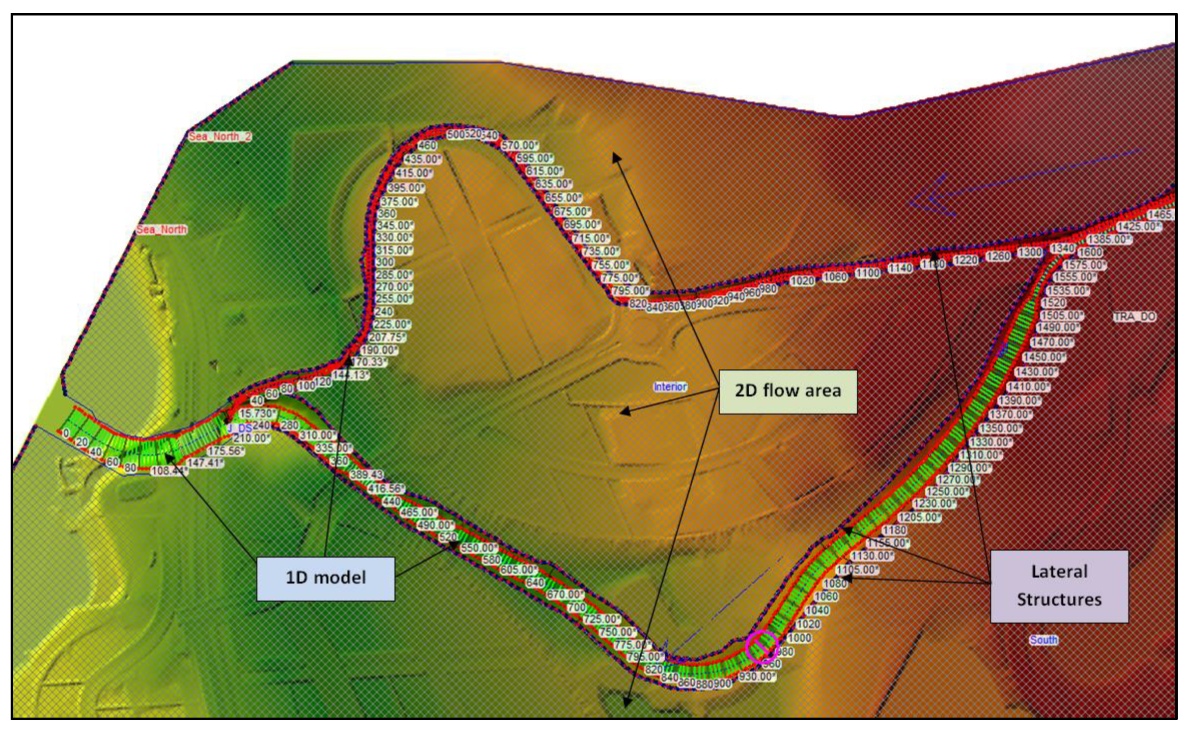
6.3. Coupling of 1D/2D Simulation Models
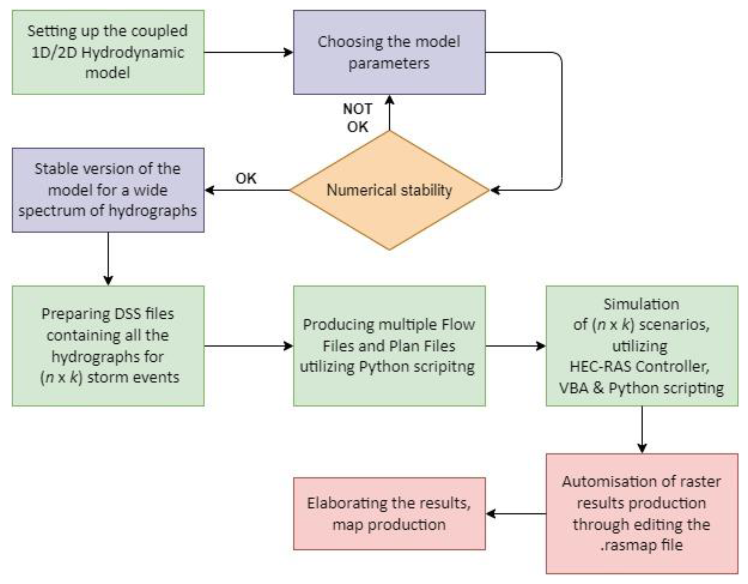
The coupling of the one-dimensional model (channels, trained sections, etc.) with the floodplains was achieved through a series of lateral weirs, placed on the highest point of the overbank. This technique provides an elegant way to assess which scenarios are selected from the full 1D simulations through the assessment of the overflowing volumes over the lateral weirs. A screenshot from the HEC-RAS software environment depicting the aforementioned 1D/2D connection is shown in
Figure 8. It should be noted that the 1D model does not serve solely as an indicator for the critical scenarios. It is an integral part of the framework, as it provides statistical description of relevant variables along the drainage network/river chainage, which can be used to quantify local hazard and resilience. For example, an important outcome of 1D analysis is the probability of overflow, which is estimated as the percentage of scenarios for which the water flows outside of the system boundaries, as defined by the lateral weirs. Lastly, given a specific metric and its respective threshold, the critical scenarios can be identified and simulated through the coupled 1D/2D model. An overall flow chart of automating the multiple 1D/2D coupled model runs is depicted in
Figure 9.
7. Statistical Processing of Simulation Outputs and Flood Hazard Mapping
7.1. Uncertainty Estimation of Flood Quantities
Typical engineering practices only provide a single estimation of flood quantities of interest per exceedance probability, which is in turn explicitly determined by the return period of the (unique) input storm event. In contrast, the outcomes of the proposed stochastic simulation framework can only be interpreted in statistical terms, which also allows for estimating the uncertainty of each quantity of interest for each return period. In general, from the sample of 100 simulated values per return period, we empirically estimate five quantiles of interest (10%, 25%, 50%, 75%, and 90%). This allows detecting the median value of each output variable, while simultaneously quantifying its uncertainty, by means of empirical confidence intervals. In fact, while the median may be considered as the most representative value for flood design purposes, engineers and stakeholders have the choice of assigning larger and, thus, more conservative design values, expressing an acceptable level of safety that also accounts for uncertainties. This option provides a powerful tool to communities and state agencies for mitigating flood hazard and communicating their design choices.
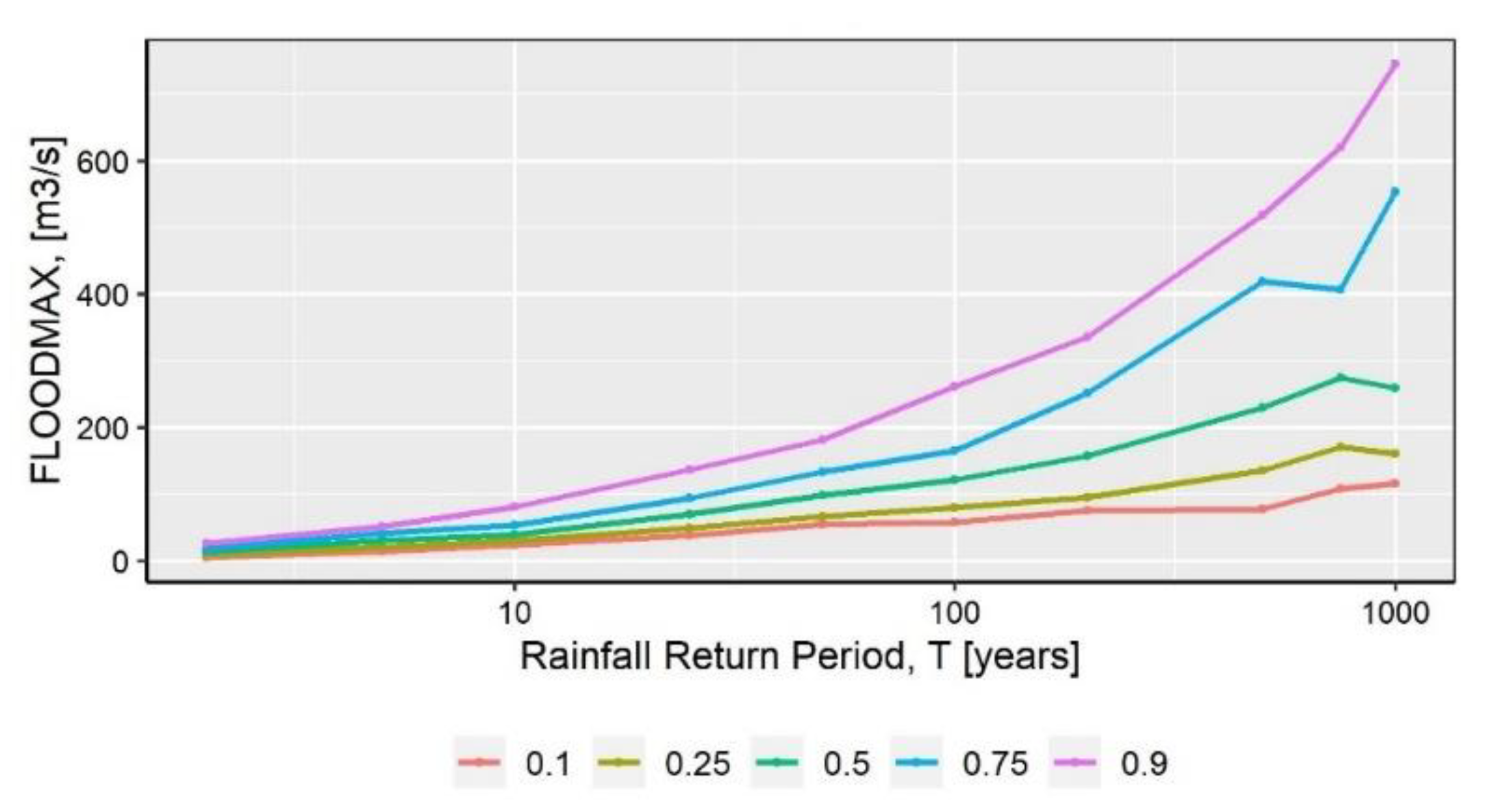
For instance, in
Figure 10, we demonstrate the statistical analysis of the 1000 simulated peak flow values (10 × 100) at the outlet of Trachones stream, which is a key outcome of the rainfall–runoff analysis. As expected, the uncertainty around the median estimation of the peak flow at the outlet increases substantially, as the return period of the 24 h rainfall increases. The same behavior is observed in all simulated quantities, including the 24 h rainfall, the temporal distribution of partial rainfall depths and, thus, hyetograph scenarios, and the uncertainty of antecedent soil moisture conditions, as quantified in terms of the
parameter (which is in turn a function of randomly varying 60 day rainfall).
7.2. Preliminary Hazard Assessment in Terms of Probability of Overflow
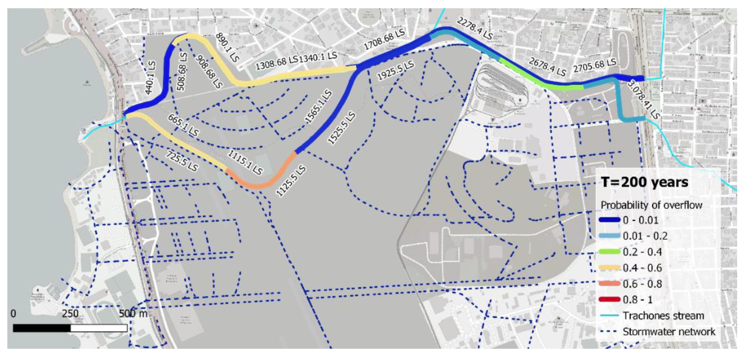
An approximative yet intelligible flood hazard metric, resulting from 1D hydrodynamic simulations, is the probability of overflowing across the drainage network, the spatial representation of which is conceptually described through the 24 lateral weirs. This was empirically estimated for each structure and each return period, by counting the number of spilling cases and dividing by the total number of flood scenarios examined per return period, i.e., 100. We highlight that, in the context of 1D simulation, the concept of spilling has a qualitative nature, because the term overflow for the closed parts of the streams translates into a maximum value of the pressure line intersecting the terrain. As the return period increases, an increasing number of overflow scenarios are encountered; thus, the flood hazard also increases. On the other hand, for 2, 5 and 10 years, the empirically derived overflow probabilities across the entire network are either zero or negligible.
In order to provide a macroscopic visual interpretation of flood hazard and its spatial distribution over the study area, we defined six probability classes based on engineering judgment, i.e., up to 1% (at most one overflow case over 100 scenarios), 1–20%, 21–40%, 41–60%, 61–80%, and 81–100%, and mapped them across the model domain, for the 10 return periods of interest. This allows easily detecting the system’s components that are systematically prone to flood events of specific frequency (defined in terms of return period of input rainfall), thus requiring further investigation and, potentially, reinforced design. For instance, as shown in
Figure 11, for the return period of 200 years, which exceeds the typical engineering design standards of 50 to 100 years, specific parts of the drainage network may be under significant hazard, while other ones exhibit low or negligible hazard.
7.3. Ranking of Overflow Scenarios
The probability of overflow is a useful yet not fully representative hazard metric, since it cannot account for the magnitude of spilling. In an attempt to provide a more comprehensive screening of the 1D hydrodynamic analysis outcomes, the overflow scenarios per return period are further classified by accounting for their relative importance. In this respect, for each scenario
(
) and return period,
, we introduce the following ranking metric:
where
is the largest of simulated overflow discharge values over the lateral weir
,
is the total number of lateral weirs (i.e.,
24), and
refers to the globally maximum overflow value over the entire model domain.
Equation (10) allows quantifying, at least in a preliminary context, the potential flood hazard caused by overflows that take place across the drainage network (more accurately, the lateral weirs). For instance, a unit value indicates that one weir exhibits the largest overflow, or that two weirs exhibit half of their maximum overflow. This metric is also used to classify the scenarios per return period in hazard terms and recognize the most significant ones. It is worth mentioning that, since the overflow components are expressed in dimensionless terms, it is possible to make comparisons among scenarios that correspond to different return periods. Consequently, we can assign a specific threshold, , to detect scenarios that are plausible to be particularly hazardous, i.e., by examining whether . In this study, we applied the ranking approach in order to select specific scenarios across different return periods for a more detailed analysis through the coupled 1D/2D analysis module of HEC-RAS.
7.4. Spatial Mapping of Flood Hazard over the Study Area
Contrary to the deterministic visualization of flood hazard, in which only a single map for each variable based on the design storm can be produced, the proposed analysis procedure offers the opportunity to statistically assess the results. In turn, this allows for an improved and significantly more informed (in terms of communicating the uncertainty) decision-making strategy.
Despite the clear advantages of the stochastic approach, reducing the plethora of simulated data to a meaningful statistic, it also comes with challenges, since the presentation of the flood metrics must ensure that (i) the end reader will not be overwhelmed by the amount of information, and (ii) the outcome will not be reduced to such extent that significant information will be lost. The latter case is the most frequent one and results in the miscommunication of uncertainty, which can in turn affect decision making on design and policy levels. This is a delicate balance, and the strategy should be the result of stakeholder engagement and consultation. This fact makes this step partially case-study-dependent.
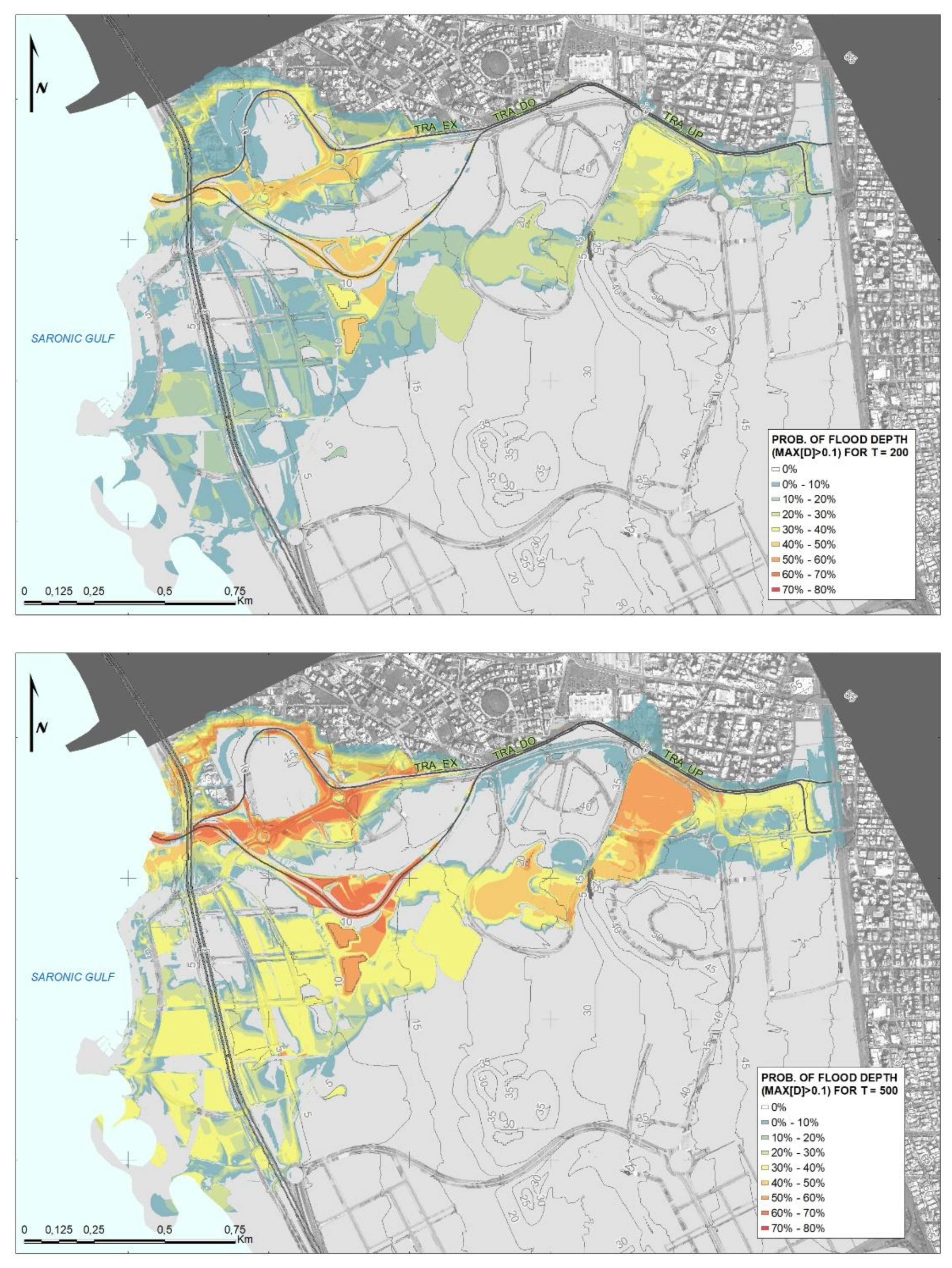
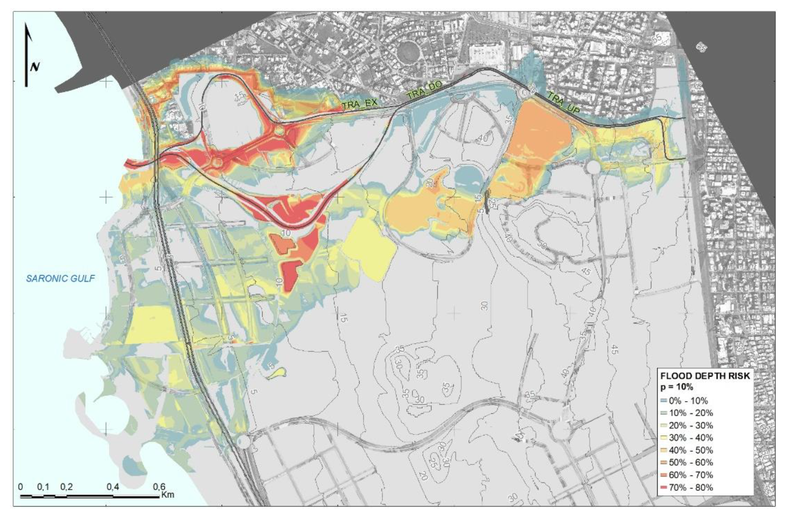
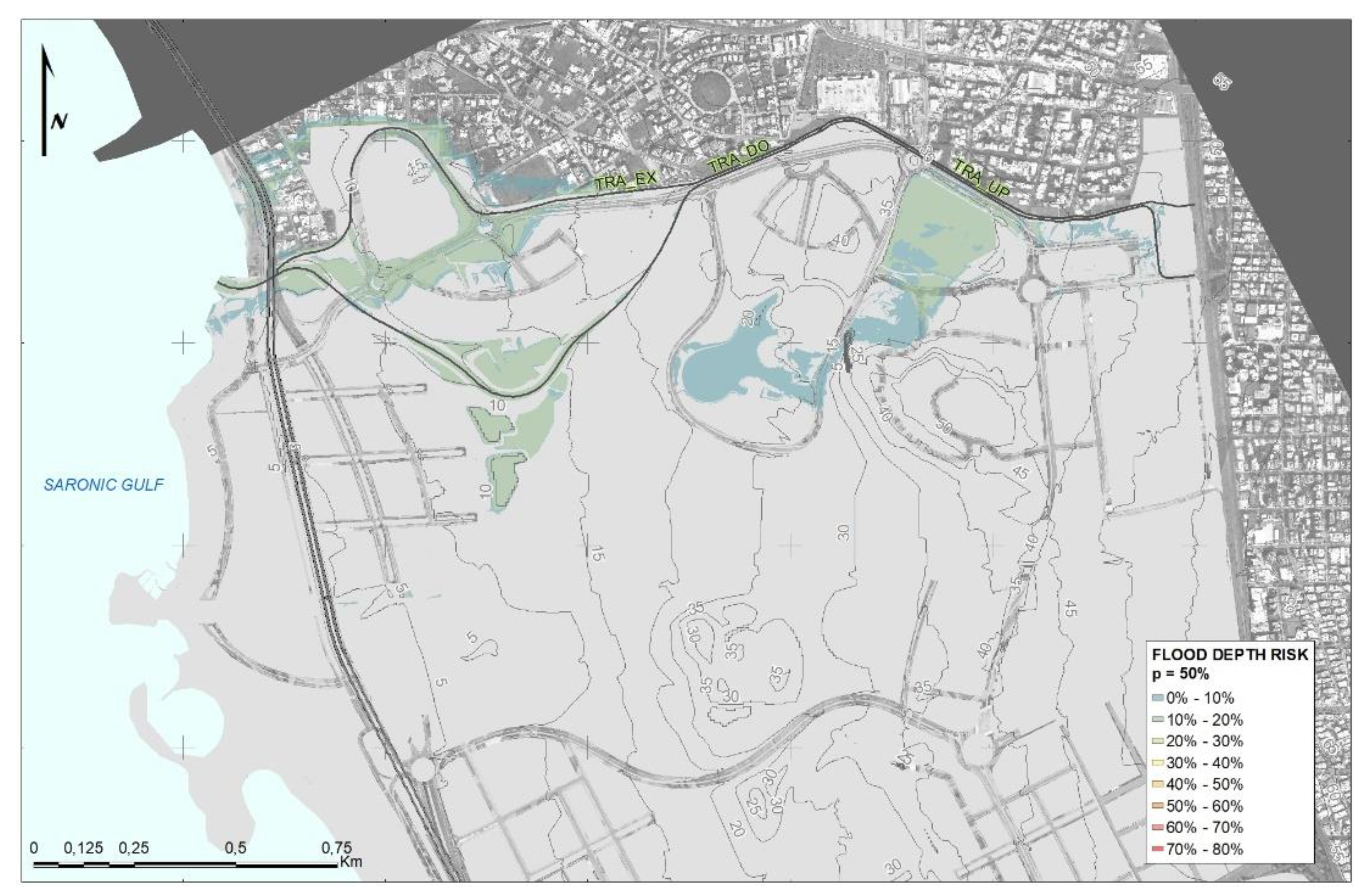
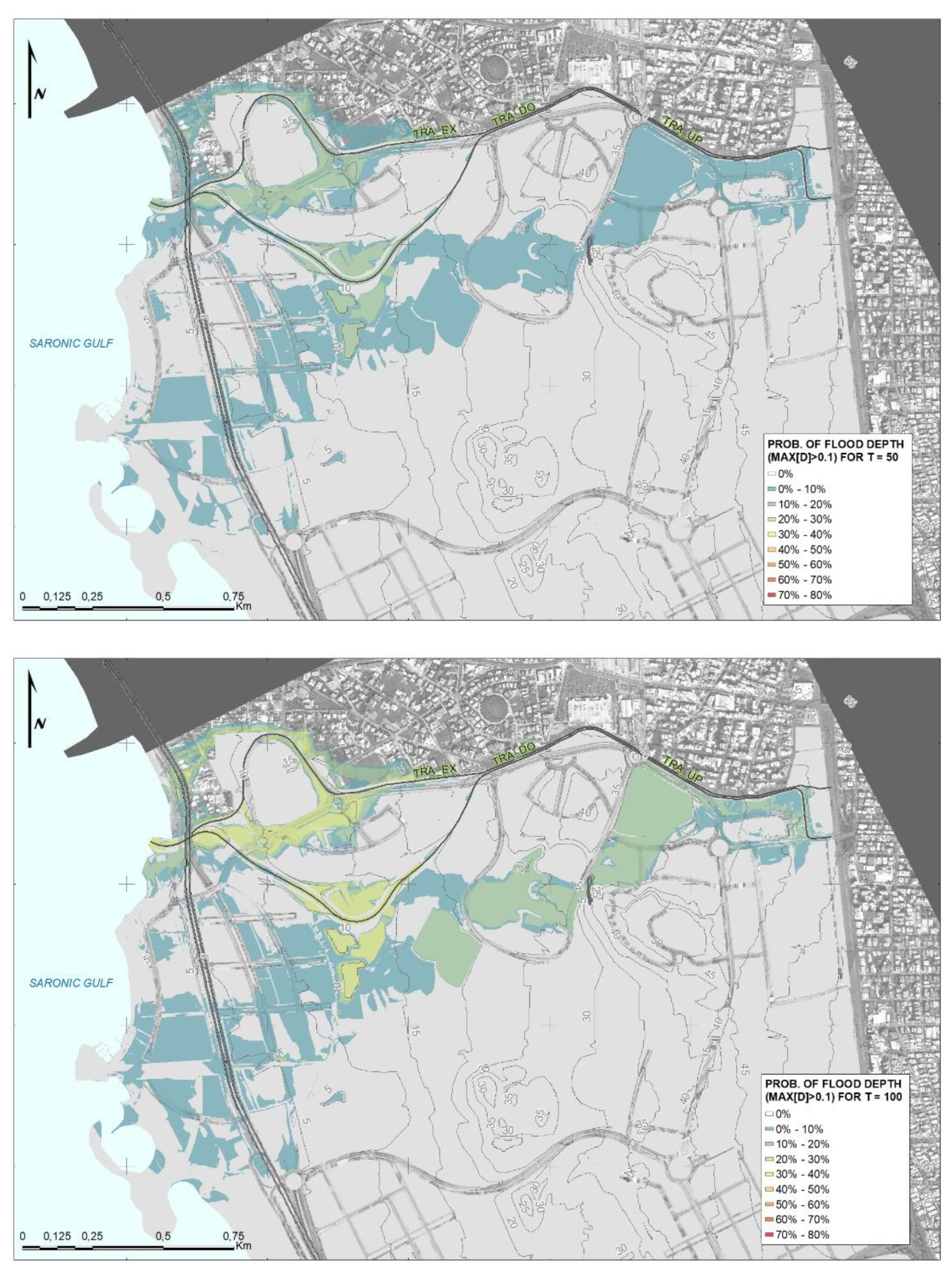
In the present study, we opted to present two metrics to quantify the flood hazard, provided that a flood depth above 0.10 m corresponds to the nominal curb height. The first one is the probability of at least one rainfall event occurring during the project lifetime (equal to 50 years) that will cause exceedance of overland flow depth of 0.1 m, under a given confidence limit. This is depicted in
Figure 12 and
Figure 13, for
= 10% and 50%, respectively. Under this depth, the roads may act as conduits, by taking advantage of their limited yet not negligible conveyance and storage capacity. If they are not incapacitated by some external force, they convey the flood waters to the nearest recipient, in positions where it is able to convey the extra volume without additional damage. The threshold of 0.10 m is introduced to the metric in order to ensure that the resulting hazard is indeed significant and, thus, the actual hazard is not overestimated.
The second metric is the probability of exceedance of the overland flow depth of 0.1 m (curb height), for a rainfall event with a given return period. This is depicted for a return period of 50 vs. 100 years in
Figure 14. Results for two additional return periods are provided in
Appendix A. This metric is particularly useful as a stress test for existing or proposed designs of lined rivers, which typically assume boundary conditions with a return period of 50 or 100 years.
8. Conclusions
In the present study, we presented a novel stochastic flood simulation framework aimed addressing the principal shortcomings of common engineering practices while retaining computational efficiency.
The core of the stochastic analysis was the recently introduced R-package anySim, for the representation of the rainfall regime over the study area and across multiple temporal scales, i.e., from the storm event scale (15 min) up to much larger scales of rainfall dynamics (i.e., annual). The model was initially applied for the generation of 10,000 years of synthetic daily rainfall (also aggregated at the 60 day scale), used as basis for the deployment of a statistical model for the annual daily maxima. Eventually, we employed the disaggregation module of anySim to generate 100 synthetic hyetographs of 15 min resolution, which capture the 10 return periods of the maximum daily rainfall (100 events per return period).
The 10 × 100 = 1000 storm events and randomly generated system states were inputs to a semi-distributed event-based hydrological simulation procedure, implemented in the Hydrologic Modeling System (HEC-HMS) environment. As explained in
Section 5, important aspects of the typical modeling procedure were adapted or improved, towards (a) expressing the inherent uncertainty of
induced by the randomly varying initial soil moisture conditions in stochastic means, also accounting for its asymptotic behavior, and (b) associating the response time of all runoff propagation mechanisms, i.e., across sub-basins, through the unit hydrograph theory, and the stream network, through the novel velocity-based approach for flood routing, against the intensity of each particular storm event. This allowed “transferring” the uncertainty of the driving meteorological processes, by means of daily and 60 day accumulated rainfall, to all aforementioned components of the overall rainfall–runoff transformation.
The stochastic outputs of rainfall–runoff simulation, i.e., 1000 flood hydrographs produced across the upstream network and the lateral sub-basins, were subsequently assigned as point inflows (boundary conditions) to a hydrodynamic simulation model of the lower drainage network (river/stream). The simulations were employed in two phases, utilizing the River Analysis System (HEC-RAS) package. Initially, we ran all scenarios in a one-dimensional (1D) analysis context, in order to represent their essential hydraulic behavior, particularly for detecting which flood scenarios result in failure. The failure mode was determined as the output of flow under pressure across the closed parts of the drainage system and the overflow of the main cross-section in the open parts of the drainage network. The failed scenarios were subsequently classified according to an empirical hazard metric, and only the most important ones were further analyzed by enabling the coupled 1D/2D simulation mode of HEC-RAS. The latter allowed representing the spatial extent of the most significant flood events, and eventually providing flood hazard maps, which is an essential background for risk-aware analyses and designs.
The overall framework embodies multiple innovations with respect to (i) handling significant components within process representation as stochastic variables, (ii) employing a modular structure that allows utilizing interchangeably freeware or open-source tools and models within each subcomponent of the modeling cascade, and (iii) integrating familiar concepts for flood engineers into a hazard-informed approach that can be communicated with stakeholders. Moreover, the resulting hazard maps can be easily combined with exposure information expressed in monetary terms. Thus, this methodology can serve as a tool to estimate flood risk and assist in the decision level and asset management.
Author Contributions
Conceptualization, A.E., C.M. and S.M.; methodology, A.E., P.D., G.P., I.T., P.K., V.B. and G.-K.S.; software, P.D., G.P., I.T. and P.K.; formal analysis, P.D., G.P., I.T., P.K., V.B. and G.-K.S.; writing—original draft preparation, A.E. and P.D.; writing—review and editing, A.E., P.D., G.P., I.T. and V.B.; supervision, C.M.; project administration, S.M. All authors have read and agreed to the published version of the manuscript.
Funding
This work was carried out as part of the project “Flood risk analysis of the proposed stormwater drainage system of the Hellinikon urban development project”, under a contract assigned to Hydroexigiantiki S.A. from Lamda Development S.A., Athens, Greece. This publication is in accordance with the related contractual provisions. Lamda Development’s encouragement to extend, validate, and apply our research in this project is appreciated. The views contained in this manuscript are of its authors and cannot be assumed to represent views of Lamda Development S.A.
Data Availability Statement
The data that support the findings of this study can be provided by the corresponding author upon request.
Acknowledgments
We are grateful to the Academic Editor, who coordinated the review procedure, and the three anonymous reviewers for their positive comments and useful suggestions, which helped substantially in improving the presentation of our work.
Conflicts of Interest
The authors declare no conflict of interest.
Appendix A
Figure A1.
Probability of depth >0.1 m (curb height), for a rainfall event with years (top) vs. 500 years (bottom).
Figure A1.
Probability of depth >0.1 m (curb height), for a rainfall event with years (top) vs. 500 years (bottom).
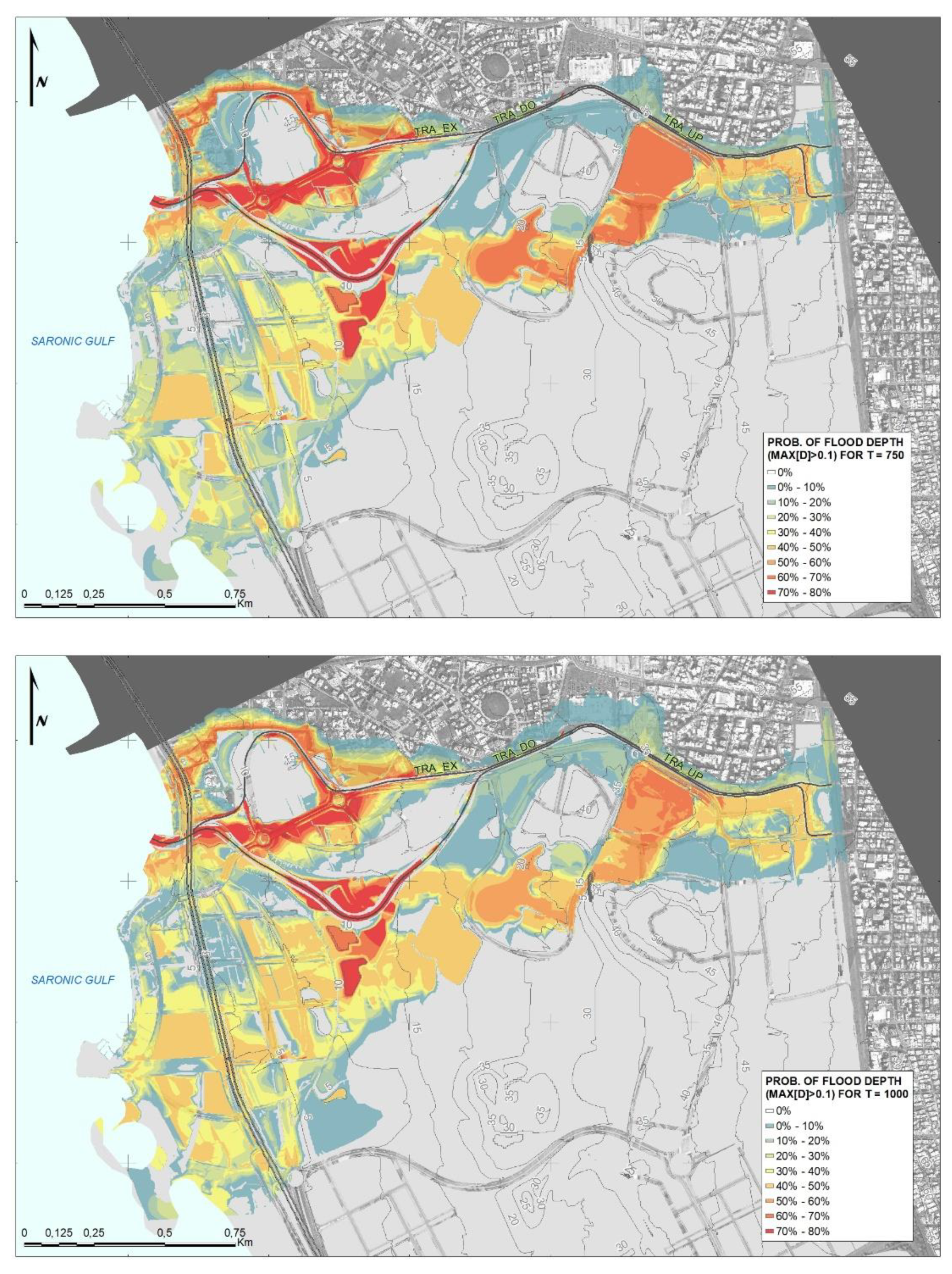
Figure A2.
Probability of depth >0.1 m (curb height), for a rainfall event with years (top) vs. 1000 years (bottom).
Figure A2.
Probability of depth >0.1 m (curb height), for a rainfall event with years (top) vs. 1000 years (bottom).
References
- Efstratiadis, A.; Koussis, A.D.; Koutsoyiannis, D.; Mamassis, N. Flood design recipes vs. reality: Can predictions for ungauged basins be trusted? Nat. Hazards Earth Syst. Sci. 2014, 14, 1417–1428. [Google Scholar] [CrossRef] [Green Version]
- Sordo-Ward, Á.; Bianucci, P.; Garrote, L.; Granados, A. How Safe is Hydrologic Infrastructure Design? Analysis of Factors Affecting Extreme Flood Estimation. J. Hydrol. Eng. 2014, 19, 04014028. [Google Scholar] [CrossRef]
- Michel, C.; Andréassian, V.; Perrin, C. Soil Conservation Service Curve Number method: How to mend a wrong soil moisture accounting procedure? Water Resour. Res. 2005, 41, 6. [Google Scholar] [CrossRef]
- Yu, D.; Yang, J.; Shi, L.; Zhang, Q.; Huang, K.; Fang, Y.; Zha, Y. On the uncertainty of initial condition and initialization approaches in variably saturated flow modeling. Hydrol. Earth Syst. Sci. 2019, 23, 2897–2914. [Google Scholar] [CrossRef] [Green Version]
- Ponce, V.M.; Hawkins, R.H. Runoff Curve Number: Has It Reached Maturity? J. Hydrol. Eng. 1996, 1, 11–19. [Google Scholar] [CrossRef]
- Alfieri, L.; Laio, F.; Claps, P. A simulation experiment for optimal design hyetograph selection. Hydrol. Process. 2008, 22, 813–820. [Google Scholar] [CrossRef]
- Krvavica, N.; Rubinić, J. Evaluation of Design Storms and Critical Rainfall Durations for Flood Prediction in Partially Urbanized Catchments. Water 2020, 12, 2044. [Google Scholar] [CrossRef]
- Michailidi, E.M.; Antoniadi, S.; Koukouvinos, A.; Bacchi, B.; Efstratiadis, A. Timing the time of concentration: Shedding light on a paradox. Hydrol. Sci. J. 2018, 63, 721–740. [Google Scholar] [CrossRef] [Green Version]
- Moreno-Rodenas, A.M.; Bellos, V.; Langeveld, J.G.; Clemens, F.H.L.R. A dynamic emulator for physically based flow simulators under varying rainfall and parametric conditions. Water Res. 2018, 142, 512–527. [Google Scholar] [CrossRef]
- Muthusamy, M.; Schellart, A.; Tait, S.; Heuvelink, G.B.M. Geostatistical upscaling of rain gauge data to support uncertainty analysis of lumped urban hydrological models. Hydrol. Earth Syst. Sci. 2017, 21, 1077–1091. [Google Scholar] [CrossRef] [Green Version]
- Bellos, V.; Papageorgaki, I.; Kourtis, I.; Vangelis, H.; Kalogiros, I.; Tsakiris, G. Reconstruction of a flash flood event using a 2D hydrodynamic model under spatial and temporal variability of storm. Nat. Hazards 2020, 101, 711–726. [Google Scholar] [CrossRef]
- Viglione, A.; Blöschl, G. On the role of storm duration in the mapping of rainfall to flood return periods. Hydrol. Earth Syst. Sci. 2009, 13, 205–216. [Google Scholar] [CrossRef] [Green Version]
- Breinl, K.; Lun, D.; Müller-Thomy, H.; Blöschl, G. Understanding the relationship between rainfall and flood probabilities through combined intensity-duration-frequency analysis. J. Hydrol. 2021, 602, 126759. [Google Scholar] [CrossRef]
- Boughton, W.; Droop, O. Continuous simulation for design flood estimation—A review. Environ. Model. Softw. 2003, 18, 309–318. [Google Scholar] [CrossRef]
- Grimaldi, S.; Petroselli, A.; Serinaldi, F. A continuous simulation model for design-hydrograph estimation in small and ungauged watersheds. Hydrol. Sci. J. 2012, 57, 1035–1051. [Google Scholar] [CrossRef]
- Winter, B.; Schneeberger, K.; Dung, N.V.; Huttenlau, M.; Achleitner, S.; Stötter, J.; Merz, B.; Vorogushyn, S. A continuous modelling approach for design flood estimation on sub-daily time scale. Hydrol. Sci. J. 2019, 64, 539–554. [Google Scholar] [CrossRef]
- Koutsoyiannis, D. Stochastics of Hydroclimatic Extremes—A Cool Look at Risk; Hellenic Academic Libraries Link.: Athens, Greece, 2021. [Google Scholar]
- Tscheikner-Gratl, F.; Bellos, V.; Schellart, A.; Moreno-Rodenas, A.; Muthusamy, M.; Langeveld, J.; Clemens, F.; Benedetti, L.; Rico-Ramirez, M.A.; de Carvalho, R.F.; et al. Recent insights on uncertainties present in integrated catchment water quality modelling. Water Res. 2019, 150, 368–379. [Google Scholar] [CrossRef]
- Gabriel-Martin, I.; Sordo-Ward, A.; Garrote, L.; García, J.T. Dependence Between Extreme Rainfall Events and the Seasonality and Bivariate Properties of Floods. A Continuous Distributed Physically-Based Approach. Water 2019, 11, 1896. [Google Scholar] [CrossRef] [Green Version]
- Paquet, E.; Garavaglia, F.; Garçon, R.; Gailhard, J. The SCHADEX method: A semi-continuous rainfall–runoff simulation for extreme flood estimation. J. Hydrol. 2013, 495, 23–37. [Google Scholar] [CrossRef]
- Makropoulos, C.; Nikolopoulos, D.; Palmen, L.; Kools, S.; Segrave, A.; Vries, D.; Koop, S.; van Alphen, H.J.; Vonk, E.; van Thienen, P.; et al. A resilience assessment method for urban water systems. Urban Water J. 2018, 15, 316–328. [Google Scholar] [CrossRef]
- Dimitriadis, P.; Tegos, A.; Oikonomou, A.; Pagana, V.; Koukouvinos, A.; Mamassis, N.; Koutsoyiannis, D.; Efstratiadis, A. Comparative evaluation of 1D and quasi-2D hydraulic models based on benchmark and real-world applications for uncertainty assessment in flood mapping. J. Hydrol. 2016, 534, 478–492. [Google Scholar] [CrossRef]
- Tsoukalas, I.; Kossieris, P.; Makropoulos, C. Simulation of Non-Gaussian Correlated Random Variables, Stochastic Processes and Random Fields: Introducing the anySim R-Package for Environmental Applications and Beyond. Water 2020, 12, 1645. [Google Scholar] [CrossRef]
- Tsoukalas, I.; Efstratiadis, A.; Makropoulos, C. Building a puzzle to solve a riddle: A multi-scale disaggregation approach for multivariate stochastic processes with any marginal distribution and correlation structure. J. Hydrol. 2019, 575, 354–380. [Google Scholar] [CrossRef]
- Tyralis, H.; Koutsoyiannis, D.; Kozanis, S. An algorithm to construct Monte Carlo confidence intervals for an arbitrary function of probability distribution parameters. Comput. Stat. 2013, 28, 1501–1527. [Google Scholar] [CrossRef]
- Tsoukalas, I. The tales that the distribution tails of non-Gaussian autocorrelated processes tell: Efficient methods for the estimation of the k-length block-maxima distribution. Hydrol. Sci. J. 2021. [Google Scholar]
- Kossieris, P.; Tsoukalas, I.; Efstratiadis, A.; Makropoulos, C. Generic Framework for Downscaling Statistical Quantities at Fine Time-Scales and Its Perspectives towards Cost-Effective Enrichment of Water Demand Records. Water 2021, 13, 3429. [Google Scholar] [CrossRef]
- USDA National Resources Conservation Service. National Engineering Handbook: Part 630—Hydrology; USDA National Resources Conservation Service: Washington, DC, USA, 2004.
- Silveira, L.; Charbonnier, F.; Genta, J.L. The antecedent soil moisture condition of the curve number procedure. Hydrol. Sci. J. 2000, 45, 3–12. [Google Scholar] [CrossRef] [Green Version]
- Hjelmfelt, A.T. Investigation of Curve Number Procedure. J. Hydraul. Eng. 1991, 117, 725–737. [Google Scholar] [CrossRef]
- Shi, W.; Wang, N. An Improved SCS-CN Method Incorporating Slope, Soil Moisture, and Storm Duration Factors for Runoff Prediction. Water 2020, 12, 1335. [Google Scholar] [CrossRef]
- Sahu, R.K.; Mishra, S.K.; Eldho, T.I.; Jain, M.K. An advanced soil moisture accounting procedure for SCS curve number method. Hydrol. Process. 2007, 21, 2872–2881. [Google Scholar] [CrossRef]
- Camici, S.; Tarpanelli, A.; Brocca, L.; Melone, F.; Moramarco, T. Design soil moisture estimation by comparing continuous and storm-based rainfall-runoff modeling. Water Resour. Res. 2011, 47, W05527. [Google Scholar] [CrossRef]
- Mishra, S.K.; Singh, V.P. A relook at NEH-4 curve number data and antecedent moisture condition criteria. Hydrol. Process. 2006, 20, 2755–2768. [Google Scholar] [CrossRef]
- Grimaldi, S.; Petroselli, A.; Serinaldi, F. Design hydrograph estimation in small and ungauged watersheds: Continuous simulation method versus event-based approach. Hydrol. Process. 2012, 26, 3124–3134. [Google Scholar] [CrossRef]
- Verma, S.; Verma, R.K.; Mishra, S.K.; Singh, A.; Jayaraj, G.K. A revisit of NRCS-CN inspired models coupled with RS and GIS for runoff estimation. Hydrol. Sci. J. 2017, 62, 1891–1930. [Google Scholar] [CrossRef]
- Hawkins, R.H. Asymptotic Determination of Runoff Curve Numbers from Data. J. Irrig. Drain. Eng. 1993, 119, 334–345. [Google Scholar] [CrossRef]
- Mishra, S.K.; Singh, V.P. SCS-CN method: Part-I: Derivation of SCS-CN based models. Acta Geophys. Pol. 2002, 50, 457–477. [Google Scholar]
- Grimaldi, S.; Petroselli, A.; Tauro, F.; Porfiri, M. Time of concentration: A paradox in modern hydrology. Hydrol. Sci. J. 2012, 57, 217–228. [Google Scholar] [CrossRef] [Green Version]
- Efstratiadis, A.; Koukouvinos, A.; Michailidi, E.M.; Galiouna, E.; Tzouka, A.; Koussis, A.D.; Mamassis, N.; Koutsoyiannis, D. Description of Regional Approaches for the Estimation of Characteristic Hydrological Quantities, DEUCALION—Assessment of Flood Flows in Greece under Conditions of Hydroclimatic Variability: Development of Physically-Established Conceptual-Probabilistic Framework and Computational Tools; National Technical Unversity of Athes: Athes, Greece, 2014. [Google Scholar]
- Papaioannou, G.; Efstratiadis, A.; Vasiliades, L.; Loukas, A.; Papalexiou, S.M.; Koukouvinos, A.; Tsoukalas, I.; Kossieris, P. An operational method for Flood Directive implementation in ungauged urban areas. Hydrology 2018, 5, 24. [Google Scholar] [CrossRef] [Green Version]
- Papaioannou, G.; Vasiliades, L.; Loukas, A.; Alamanos, A.; Efstratiadis, A.; Koukouvinos, A.; Tsoukalas, I.; Kossieris, P. A Flood Inundation Modeling Approach for Urban and Rural Areas in Lake and Large-Scale River Basins. Water 2021, 13, 1264. [Google Scholar] [CrossRef]
- Natural Resources Conservation Service (NRCS). Chapter 16: Hydrographs. In National Engineering Handbook: Part 630—Hydrology; Natural Resources Conservation Service (NRCS): Washington, DC, USA, 2007. [Google Scholar]
- Risva, K.; Nikolopoulos, D.; Efstratiadis, A. Distributed hydrological modelling using spatiotemporally varying velocities. In Proceedings of the EGU General Assembly 2020, Online event, 4–8 May 2020. EGU2020-13402. [Google Scholar]
Figure 1.
Cascade of models and exchange of input and output data within the hybrid stochastic simulation framework. In the present study, we use , and .
Figure 1.
Cascade of models and exchange of input and output data within the hybrid stochastic simulation framework. In the present study, we use , and .
Figure 2.
Hydrological modeling system of Trachones stream.
Figure 2.
Hydrological modeling system of Trachones stream.
Figure 3.
Maximum daily (24 h) rainfall intensity, (mm/h) vs. return period (years) (including confidence levels).
Figure 3.
Maximum daily (24 h) rainfall intensity, (mm/h) vs. return period (years) (including confidence levels).
Figure 4.
Synthetically generated 24 h design hyetographs (time interval 15 min), grouped by return period (years) (100 synthetic hyetographs per ).
Figure 4.
Synthetically generated 24 h design hyetographs (time interval 15 min), grouped by return period (years) (100 synthetic hyetographs per ).
Figure 5.
Example of adjusting reference : (a) mapping to non-exceedance probability of 60 day rainfall through the probabilistic function (4); (b) mapping to 60 day rainfall through the generalized formula in Equation (5).
Figure 5.
Example of adjusting reference : (a) mapping to non-exceedance probability of 60 day rainfall through the probabilistic function (4); (b) mapping to 60 day rainfall through the generalized formula in Equation (5).
Figure 6.
Simulated daily runoff from 1955 to 2019, through the NRCS-CN approach for , by considering constant and varying (adjusted to 60 day rainfall) .
Figure 6.
Simulated daily runoff from 1955 to 2019, through the NRCS-CN approach for , by considering constant and varying (adjusted to 60 day rainfall) .
Figure 7.
Scatter plots of daily runoff estimated through the proposed approach vs. the continuous simulation scheme by Mishra and Singh [
38] for reference values (
a)
, and (
b)
.
Figure 7.
Scatter plots of daily runoff estimated through the proposed approach vs. the continuous simulation scheme by Mishra and Singh [
38] for reference values (
a)
, and (
b)
.
Figure 8.
Screenshot of a section from the coupled 1D/2D model (as shown in the GUI of HEC-RAS Geometry Editor).
Figure 8.
Screenshot of a section from the coupled 1D/2D model (as shown in the GUI of HEC-RAS Geometry Editor).
Figure 9.
Methodology flow chart of the multiple coupled 1D/2D hydrodynamic model runs.
Figure 9.
Methodology flow chart of the multiple coupled 1D/2D hydrodynamic model runs.
Figure 10.
Probabilistic plots of simulated peak flow values at the outlet of Trachones stream.
Figure 10.
Probabilistic plots of simulated peak flow values at the outlet of Trachones stream.
Figure 11.
Mapping of probability of overflow classes across the 24 lateral structures of lower Trachones drainage network, for 200 years.
Figure 11.
Mapping of probability of overflow classes across the 24 lateral structures of lower Trachones drainage network, for 200 years.
Figure 12.
Mapping of flood depth hazard (10% confidence limit).
Figure 12.
Mapping of flood depth hazard (10% confidence limit).
Figure 13.
Mapping of flood depth hazard (50% confidence limit).
Figure 13.
Mapping of flood depth hazard (50% confidence limit).
Figure 14.
Probability of depth >0.1 m (curb height), for a rainfall event with years (top) vs. 100 years (bottom).
Figure 14.
Probability of depth >0.1 m (curb height), for a rainfall event with years (top) vs. 100 years (bottom).
Table 1.
Uncertainties for each module considered in the present study.
Table 1.
Uncertainties for each module considered in the present study.
| Weather Generation | Rainfall–Runoff Transformation |
|---|
- ○
Statistical uncertainty of annual rainfall maxima
| - ○
Antecedent soil moisture conditions
|
- ○
Temporal distribution of storm events
| - ○
Runoff routing over sub-basins
|
| | - ○
Hydrograph routing along the stream network
|
Table 2.
Accumulated rainfall (mm) for various scales of aggregation at Hellinikon station and correspondence with soil moisture conditions over the study area.
Table 2.
Accumulated rainfall (mm) for various scales of aggregation at Hellinikon station and correspondence with soil moisture conditions over the study area.
Rainfall
Quantile | Soil Moisture
Conditions | Scale of Aggregation, n |
|---|
| 5 Days | 15 Days | 30 Days | 60 Days |
|---|
| 1% | Very dry | 0.0 | 0.0 | 0.0 | 0.1 |
| 10% | Dry (AMC I) | 0.0 | 0.0 | 0.0 | 1.9 |
| 50% | Normal (AMC II) | 0.0 | 4.9 | 16.7 | 43.2 |
| 90% | Wet (AMC III) | 15.7 | 42.6 | 78.3 | 139.6 |
| 99% | Very wet | 55.1 | 97.5 | 153.9 | 220.3 |
| 99.9% | Extremely wet | 109.9 | 179.6 | 212.0 | 283.7 |
Table 3.
Statistical comparison of nonzero runoff data through the NRCS-CN approach for , by considering constant and varying (adjusted to 60 day rainfall) CN.
Table 3.
Statistical comparison of nonzero runoff data through the NRCS-CN approach for , by considering constant and varying (adjusted to 60 day rainfall) CN.
| | | |
|---|
| Average (mm) | 1.43 | 3.30 |
| Standard deviation (mm) | 3.90 | 5.43 |
| Coefficient of skewness | 7.15 | 4.81 |
Table 4.
Adjustment factors to reference time of concentration.
Table 4.
Adjustment factors to reference time of concentration.
(Years)
| |
|---|
| 10% | 25% | 50% | 75% | 90% |
|---|
| 2 | 1.25 | 1.23 | 1.21 | 1.18 | 1.16 |
| 5 | 1.04 | 1.02 | 1.00 | 0.98 | 0.95 |
| 10 | 0.95 | 0.92 | 0.89 | 0.87 | 0.84 |
| 25 | 0.85 | 0.82 | 0.79 | 0.75 | 0.72 |
| 50 | 0.80 | 0.76 | 0.72 | 0.68 | 0.64 |
| 100 | 0.75 | 0.71 | 0.66 | 0.61 | 0.57 |
| 200 | 0.71 | 0.66 | 0.61 | 0.56 | 0.51 |
| 500 | 0.66 | 0.61 | 0.55 | 0.49 | 0.44 |
| 750 | 0.64 | 0.59 | 0.53 | 0.47 | 0.41 |
| 1000 | 0.63 | 0.58 | 0.51 | 0.45 | 0.39 |
| Publisher’s Note: MDPI stays neutral with regard to jurisdictional claims in published maps and institutional affiliations. |
© 2022 by the authors. Licensee MDPI, Basel, Switzerland. This article is an open access article distributed under the terms and conditions of the Creative Commons Attribution (CC BY) license (https://creativecommons.org/licenses/by/4.0/).


 ,
, 


