Minimum Cost Water Yield Strategy for Multiple Sources Water Distribution System

Abstract

Minimizing water supply costs has always been the goal of water companies. However, it is not an easy task to minimize costs and meet customers’ water pressure needs in a water supply system with multiple sources and different unit costs of water discharge. In this paper, we develop a search method that incorporates the concepts of local search and steepest descent. First, we establish the discharge pressure of each water source as a variable and start searching the neighborhood for a feasible initial solution. The steepest descent concept is then used to find the most cost-effective solution in the neighborhood, before the initial solution is updated. We then iterate the search as described above until either the constraint is met or the amount of cost variation reaches an acceptable level. A simple example is used to explore the optimal solution characteristics. This is then followed by an analysis of a practical water supply system with up to six water sources. Compared with the original operation model, the optimized result can save 15.6%, 9.0%, and 12.7% of the total cost of water supply during off-peak, normal, and peak periods, respectively. We use the commonly used hydraulic analysis software EPANET to build different functional valve classes to satisfy various constraints for the purpose of simplifying the optimized search codes automatically. This method uses low levels of computational resources to obtain an acceptable and reasonable solution in a short time.

1. Introduction

A water utility manager often faces a conflict between operational performance and service quality. For example, the water supply pressure at the customer end is not in line with the operational performance, and higher water supply pressure results in high leakage and higher water supply costs. Therefore, in pursuit of the goal of maximizing operational performance, it is necessary to meet the most basic service quality, that is, to meet the minimum acceptable water pressure for customers. For a water distribution system (WDS) with a single water source (water treatment plant), this can be easily achieved by adjusting the discharge pressure of the water source. However, for a multiple loading WDS, each water treatment plant (WTP) has a different water unit cost due to variations in raw water quality, drinking water quality standards, water purification procedures, and site elevation, etc. To meet the customer’s water pressure demand and minimum cost simultaneously, we should appropriately allocate the water discharge from each plant.

Take the Kaohsiung system of the Taiwan Water Corporation (TWC) as an example. The system supplies about 1.28 million cubic meters of domestic water to the Kaohsiung area from six WTPs daily. Due to the high hardness and total dissolved solids (close to 300 mg/L and 500 mg/L, respectively, during the dry season) in the raw water of the Gaoping River, four of the WTPs were contracted out to professional water treatment companies for additional advanced water treatment procedures, such as pellet softening or reverse osmosis, in order to meet the public’s demand for drinkability. TWC contracted with each outsourced operator different water capacities and different water unit price terms according to the different raw water quality and freshwater quality requirements. When the system nodal pressure does not meet the minimum requirements for customers, the TWC must direct the water discharge from each WTP in an effective and less costly manner. This paper takes the minimum water supply cost of the system as the objective function in an optimization problem of WDS operations and tries to develop a search method to find a practically feasible water allocation strategy to provide as a reference in operators’ decision making.

Before solving the WDS optimization problem, we need to understand the nature of the problem, set the objective (function), constraints and decision variables, and then choose the network simulation and optimization method, so that the optimum solution can be obtained after calculation. The network simulation can be solved by listing all the explicit mathematical formulas according to the conservation of mass and energy of the system. Once the WDS is larger or has more complex components (e.g., adding valves, pumps, etc.), not only is it difficult to formulate, but the calculation process is also prone to errors. After the development of pipe network analysis software such as KYPipe and EPANET, it is not only the hydraulic analysis that can be calculated, but also the extended period simulation (EPS), including water quality, which has been adopted by many researchers.

Optimization algorithms are generally classified as deterministic or stochastic methods. For deterministic methods, the same answer is obtained for each calculation if the initial conditions are identical. Conversely, the calculation process for stochastic methods involves some randomness such that individual results will differ, even if it starts from the same initial point [1]. In the case of a small WDS, mathematical deterministic methods such as linear programming (LP) [2], nonlinear programming (NLP) [3], mixed integer nonlinear programming (MINLP) [4], and dynamic programming (DP) [5,6], can be used to solve most single-objective optimization problems.

Due to the increasing complexity of WDSs and the increasing emphasis on multi-objective optimization, including energy saving, water quality, stable water supply, etc., deterministic methods are difficult or impossible to solve. Since the 1990s, meta-heuristics that simulate natural phenomena and use a certain degree of weighting, random, and local search have become popular [1], including the evolutionary algorithm (EA) [7], differential evolution (DE) [8], ant colony optimization (ACO) [9], adaptive search algorithm (ASA) [10], simulated annealing (SA), harmony search (HS), and particle swarm optimization (PSO), etc. Among these meta-heuristics, evolutionary algorithms (EAs) that can solve a variety of water resources problems have become the mainstream, and genetic algorithms (GAs) are the most popular [11]. In recent years, there has been a growing trend among genetic algorithms of solving WDS multi-objective optimization with the non-dominated sorting genetic algorithm (NSGA-II) [12]. Often, these studies show that algorithms are more accurate and efficient than those used in previous studies without explaining why the selected algorithm performs better in the specified test network and without understanding the underlying principles behind the algorithm’s performance [1,13].

Evidence from the literature shows that the combination of meta-heuristic algorithms and network simulators (such as EPANET) is not sufficient for the computational efficiency of large-scale WDSs [14]. To solve the above problem, several authors have studied how to reduce the computational workload to provide the best solution in real time, for example, by directly analyzing the complex network simulation using the artificial neural network (ANN) combined with the optimization method [8], or by simplifying network simulation to accelerate computation, using, for instance, interpretive structural modelling (ISM) [15]. Another method has been to simplify the full model of the WDS in the form of a reduced model (RM) [16]. In the latter study, the author simplified the water supply system with 867 nodes and 987 pipelines down to a reduced model (RM) with only 77 nodes and 92 pipelines, and, as a result, the simulation time was reduced by about 15 times.

Energy consumption in the water supply system is mainly due to long pumping distances and resistance to gravity [17]. In the former, energy consumption is caused by the friction of the pipe wall when the water is flowing. In the latter, energy provides head to the process of delivering clean water to the customer or delivering raw water to the water treatment plant. The operating costs of the pump include energy consumption costs and maintenance costs [13]. We can usually estimate the energy cost of a pump using the pump’s runtime, energy efficiency, and time tariff. Recently, a trade-off between water quality goals and pump operating costs has been found to be conflicting [18]. The more energy the pump consumes, the better the water quality. Conversely, limiting the energy consumed by the pump will cause the water quality to deteriorate. Similarly, water leakage and pump operating costs have been identified as conflicting goals. Optimization results show that pumping at night will minimize the energy cost of the pumps due to the cheaper off-peak tariff. The pressure in the system is higher at this time, so more leakage will occur [19,20].

The literature on water source cost and water treatment cost optimization is relatively sparse when compared to energy saving studies. The earliest consideration of water source cost and water treatment cost optimization is the particular qualities of the WDS; due to the unit cost of water from each water treatment plant being different, it is necessary to properly arrange the water from each plant to achieve the minimum total system cost. Simple multi-quality WDSs often uses explicit mathematical formulations to solve hydraulic analysis and deterministic optimization methods to solve minimum cost [21,22,23]. As the complexity of the system increases, some scholars have used the simplified model of interpretive structural modelling (ISM) for hydraulic analysis [15].

Considering the cost and water quality of multi-objective optimization, GA is often used to easily find the local optimum, but the global optimum requires more effort, so some scholars also combine this with the deterministic optimization method of mixed integer linear programming (MILP) in order to improve computational efficiency [24]. In practice, WDS operations also face various problems and solutions. For example, in the case of power limitation (insufficient water supply), the EPANET simulator and the genetic algorithm GA are combined in the MATLAB framework to solve the water supply method that meets the demand of the consumer as much as possible [25]. When water shortages occur and intermittent supply is required, the combination of the nondominated sorting genetic algorithm II (NSGA II) and the water network tool for resilience (WNTR) allows for an equitable supply of water based on demand and ensures service reliability [12].

The main problem in applying optimization methods to real WDSs is how to obtain an approximate solution in a reasonable time [1,11]. For many water resources problems, the global optimal solutions are usually unknown, so the allowable computational workload is usually determined in advance and the best solution is found within a given computational time [11]. In previous studies, engineering principles or empirical judgments are often used to improve the efficiency and correctness of algorithms. These include, for example, choosing pumps with better energy efficiency to reduce overall system energy costs [26], encouraging public utility companies to turn on the pumps in order of pumping cost [3], and ensuring that the diameter of the pipe with the maximum head loss is increased to the next commercial size to meet the minimum head requirement at the demand node [27]. When solving pumping cost minimization problems using mixed integer nonlinear programming, direct search methods are more suitable than gradient-based methods or Newton-like methods [28]. Finding the best solution directly using cost gradient technology with lower computing requirements is suitable for public utility decision-making [29].

In this paper, we try to use a local search method to test different sites and adopt the most cost-effective one as the search direction. Then, the next iteration of the search is continued until the minimum pressure of the nodes in the WDS is acceptable to the customers. This method refers to the concepts of local search and gradient descent, which involve searching step by step in the most feasible direction of cost reduction until the nodal pressure constraint is violated, so that the local optimum or near global optimum is obtained.

2. Methodology

The flow in the network must meet the conservation of mass and energy, as well as the flow and head-related constraints, and is a restricted optimization topic. To find the optimal solution to a constrained problem, we generally use an appropriate mathematical programming method after listing all system conditions and the optimization objectives, and automatically iterate and converge to the optimal solution using a computer program that performs the optimization process. Users do not need to explore physical characteristics. The optimal solution will naturally meet the set system conditions [30].

The case of the network discussed in this paper includes loops and branches. Since the head loss of the pipes is nonlinear, the optimization process may also be nonlinear. Thus, it is not easy to solve the problem by iterative linear programming, but the solution can be solved by nonlinear programming. There are two general methods when it comes to optimization for nonlinear programming. One of these is the direct method, and the other is the indirect method. The indirect method is a necessary condition for solving the optimal solution or a stationary condition. If the answer does not fit all the feasible conditions, the optimum solution may fall on the boundary of some constraints, and a complementary slackness must be introduced to distinguish the combinations of various equations and inequalities, which can easily exceed the computational capacity of the computer when the network is complex. The direct method, or search method, is generally used to find the direction and step of a better solution for the current feasible solution in the hyperplane under the constraints, before it proceeds step by step to find the maximum or minimum solution. In this paper, we adopt this approach to ensure the progressive improvement of the solution.

Since the network might be extensive and complex, this study applies the simulation-optimization method to improve the efficiency of the calculation. After using the local search to modify the water discharge strategy of each WTP, the strategy is sent to the network hydraulic calculation mode to directly simulate the flows of all pipes and nodal heads. After this, the simulation results are sent back to the search mode to determine the feasibility of the strategy, calculate the total water supply cost, and repeatedly modify the water discharge from the WTP. As mentioned above, a local search method was developed to determine the lowest total cost operation strategy for each WTP. To confirm the correctness and efficiency of this search method, we use the uniform grid sampling procedure (UGSP) [31] to compare the solution.

2.1. Problem

In this paper, we search for the operation strategy of the WDS, and this topic can be expressed as the following optimal proposition.

2.1.1. Objective function

min Z

$$Z={{\displaystyle \sum }}_{p=1}^{NP}{C}_p\left(Q_p\right)Q_p$$

(2)

where,

Z: total cost of water supply for all WTPs per day (or per hour);

$NP$: number of WTPs in the WDS;

p: WTP number,$p=1,\dots ,NP$;

$C_p\left(Q_p\right)$: unit cost of water discharge from the p^th WTP;

$Q_p$: the water discharge of the p^th WTP per day (or per hour).

Major factors leading to increased costs include climate change, improved service levels, significant investments in infrastructure expansion, renewal and asset maintenance, and continuous improvements in regulations and standards, etc. [32]. In response to environmental changes, the quality of raw water is deteriorating, and the water companies are unable to treat it due to the existing technical capacity. They are often contracted to professional water treatment companies for advanced water purification to meet drinking water quality standards. These WTPs with advanced treatment have higher water supply costs than WTPs with only traditional treatment. Different WTPs have different unit costs. The water company must allocate the appropriate discharge from these plants to meet the minimum water pressure requirements of customers and to minimize the overall cost of the WDS.

This model assumes steady-state conditions and solves the water distribution strategy for each WTP, in turn minimizing the cost of the WDS in a single period. The total water supply (which includes customer demand and system leakage) of the system is fixed during the entire period. The operating costs of a WTP include water source costs, treatment costs, pumping costs, maintenance costs, personnel costs, depreciation costs, and loan interest, etc. Among them, personnel costs, depreciation costs, and loan interest are not directly related to the water output scheduling strategy of the WTP in this study, so they can be ignored. The rest of the cost are described as follows:

(1)

Water source costs: This generally refers to all costs before raw water enters the WTP, including the cost of purchasing raw water, equipment maintenance costs, and water losses, etc.

(2)

Treatment costs: This refers to all the costs after the raw water enters the WTP, goes through each water purification process, and the produced water enters the tank, including the cost of water purification chemicals, the cost of wastewater and sludge treatment, the cost of electricity used in the plant, equipment maintenance costs, and water losses, etc.

(3)

Pumping costs: This refers to the cost of pumping water from the WTP to the customer (including the related booster station), including energy costs, equipment maintenance costs, and water losses, etc.

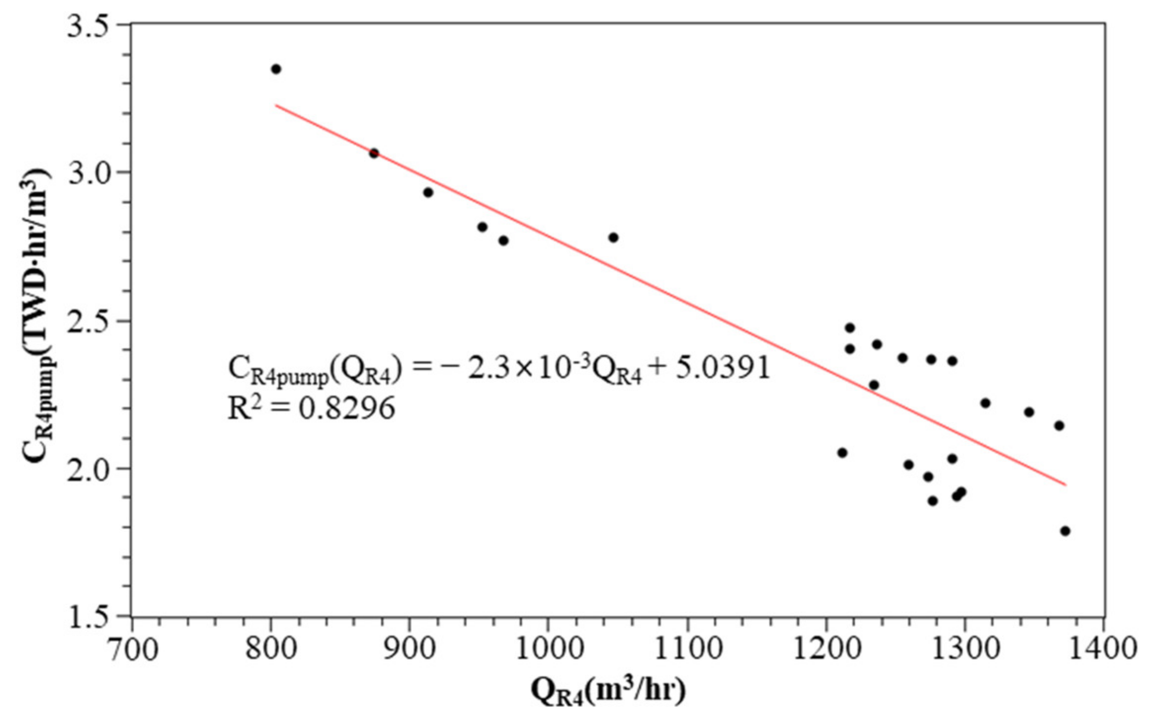
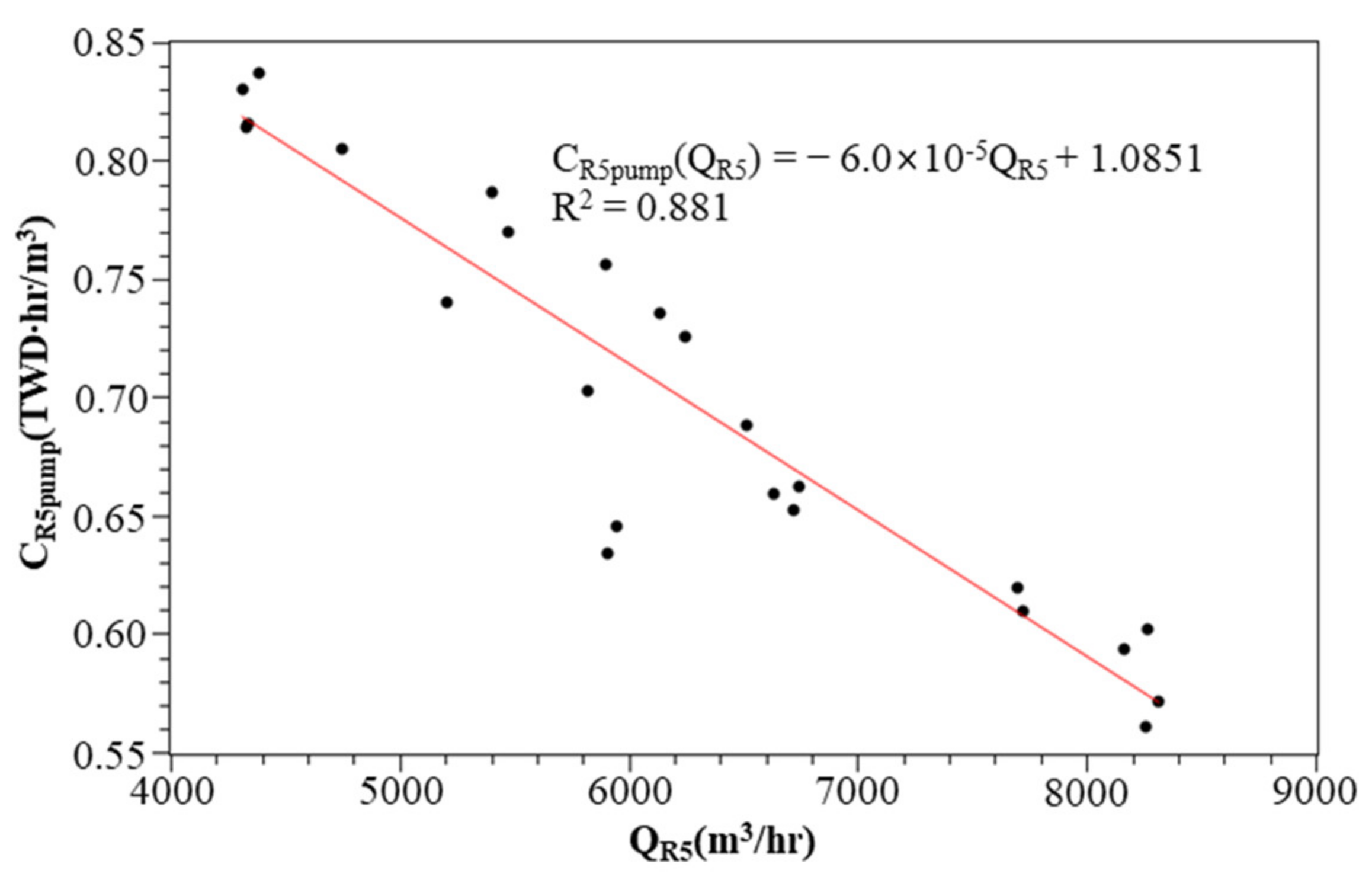
The unit cost of water from a WTP includes the fixed cost and the variable cost. The fixed cost here means that the unit cost is a fixed value and does not vary with the amount of water discharged. It can be determined by referring to the water company’s annual operating report. The variable cost is a unit cost that varies with the amount of water discharged. Depending on the elevation of the WTP, there are two types of water supply: gravity and pumped. When relying on gravity water supply only, the unit cost of water from the WTP is only a fixed cost, mainly for water source and treatment. When it is necessary to supply water by pump, the variable cost of pumping is required in addition to the fixed cost. The variables related to the pumping cost are head, flow, and energy efficiency. A WTP is usually equipped with multiple pumps of different specifications for combined discharges. Since it is not easy to find out the total energy efficiency, the pumping cost used in this study is estimated based on the actual recorded water discharge and electricity consumption. The process is as follows:

(1)

Collect the hourly water discharge and electricity consumption of the WTP for 24 h a day.

(2)

Divide the hourly electricity consumption by the water discharge to get the unit water consumption for that hour.

(3)

The average price per kWh is obtained by dividing the total amount of tariffs paid in the year by the total kWh used in the year, without distinguishing between peak and off-peak tariffs.

(4)

Multiply the hourly electricity consumption by the average price per kWh to get the hourly electricity rate.

(5)

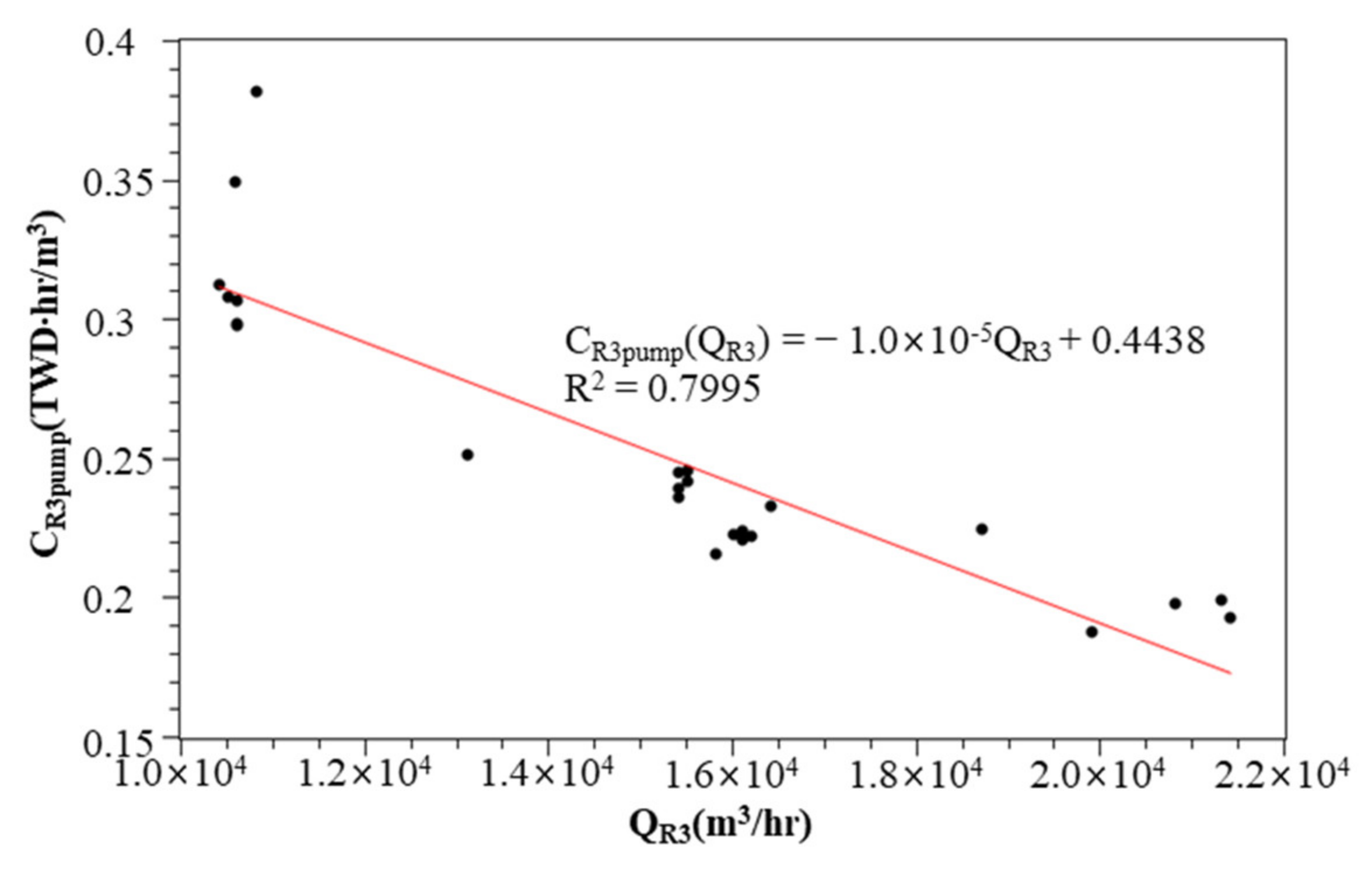
Using the hourly water discharge as the X-axis and its tariff as the Y-axis, plot the scatter diagram and fit the data with linear, quadratic, or higher order functions.

(6)

After checking these fitting functions, it is found that the fitting results of the secondary functions (and above) may differ significantly in the two extreme cases of no water and maximum water discharge. A more reasonable linear function is used to estimate the cost of electricity consumption for different water discharges.

A demonstration of the above process is shown in case 2 of this paper.

2.1.2. Constrains

The water supply system is subject to hydraulic constraints (e.g., mass conservation and energy conservation) to maintain a steady state, usually in the form of implicit constraints which can be solved by Newton’s method for nonlinear simultaneous equations or by WDS modeling tools (e.g., EPANET (Rossman 2000), KYPIPE (Wood 1980)) that are forced to be satisfied [1]. In recent years, the commonly used hydraulic simulator EPANET can also simulate water quality changes in the WDS, but, as a result, the calculation burden is increased. To reduce the computational workload of these simulations, some scholars have also replaced EPANET with an artificial neural network (ANN) as a hydraulic and water quality simulator [8]. This paper does not deal with water quality simulation, and EPANET can easily solve the results of WDS hydraulic stimulation. It has various valve modules built-in, so we can directly create a specific valve module and perform a hydraulic simulation to present the results of various hydraulic constraints, such as, for example, the maximum water discharge from the WTP can be controlled by the flow control valve (FCV), or the minimum water discharge from the WTP cannot be negative and can be controlled by the check valve (CV), etc. Other constraints are described below.

The water discharge limits of each WTP are

$$Q_p^{max}\ge Q_p\ge 0$$

(3)

where,

$Q_p^{}$: water discharge from the p^th WTP;

$Q_p^{max}$: design capacity of the p^th WTP.

The head limits at each demand node i are

$$H^{max}\ge H_i^{}\ge H^{req}$$

(4)

where,

$H_{}^{max}$: maximum head allowed at the demand node;

$H_{}^{req}$: minimum head allowed at the demand node.

The maximum head H^max at the demand node depends on the strength of the pipeline, considering the effect of the water hammer in the pipeline, which in practice is usually 1.5 times the actual maximum water supply pressure. In addition, to reduce water leakage, the maximum pressure at the node must be controlled below a specific value [1]. A “perfect” domestic water supply equipment can reduce the necessary water head H^req at the demand side without affecting the convenience of the customer through the use of, for instance, a receiving tank on the ground floor or in the basement in which freshwater is stored and pumped to the roof tank, and then gravity fed from the roof tank to each floor. This paper sets the minimum necessary head H^req = 10 m at the demand side, considering “perfect” water supply equipment at the customer end.

2.1.3. Decision Variables

$H_p^{}$: water head from the p^th WTP.

Usually, water supply systems have only a few WTPs. Take the Kaohsiung water supply system, the largest and most complex in Taiwan as an example, in which there are only six WTPs for domestic use, and so in this case there are only six decision variables, rather than the thousands of decision variables that are a challenge for general network design optimization. The search space of the decision is one of the future research challenges for WDS design optimization [1]. To simplify the search space, variable discretization is used as an important strategy. In this paper, we select the head of water from the WTP as the decision variable. Although it is theoretically a continuous value, we set a discrete value of appropriate size in the search method to shorten the solving time and reduce the chance of missing the extreme value.

2.2. Optimization Based on the Concept of Local Search

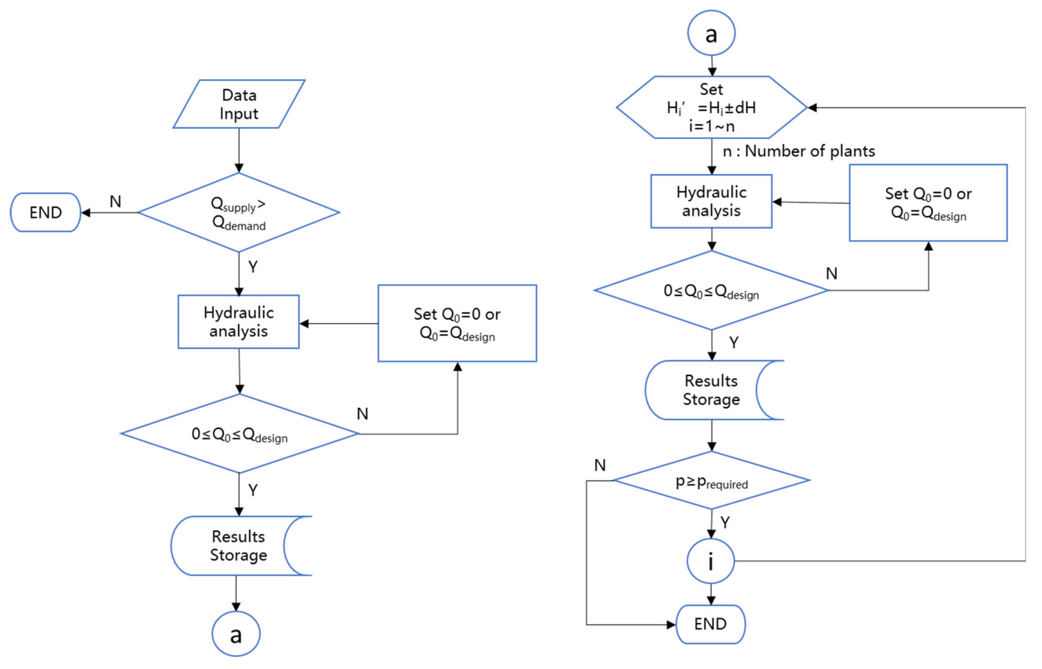
Referring to the alternative variable search [33] mentioned in Smith et al.’s book, the approach is to fix (n − 1) variables out of n decision variables, search for the minimum objective function only for a single variable, and then switch to search for another variable when the minimum value of that single variable is found. The relationship between flow and head in the WDS is nonlinear. If we search for a single variable until the minimum value is reached, it may be affected by the non-linear characteristics, resulting in the search process possibly falling into a local optimum and failing to find the near global optimum. Therefore, this paper slightly modifies the above-mentioned search by incorporating the concepts of local search and steepest descent. In a multi-source water supply system with a known feasible initial solution, the discharge pressure or flow of each WTP is used as a decision variable, and the discharge pressure or flow is added or subtracted by a slight difference according to its neighborhood, testing each point in the neighborhood one by one. Once the point that has the most significant improvement to reduce the total cost is found, it is then set as the basic value. Next, following the above process to carry out the next iteration of search, it is necessary to test until the constraints are reached. In this way, we can find the best water discharge strategy. Though this search method is slightly inefficient, due to the very limited number of decision variables, dynamically varying the step size of searching can significantly reduce the number of adjustments and make it possible to find the optimal operation strategy in a very short computation time. The computer program for performing the search is easy to code and extremely feasible in practice. The related process is explained in detail below.

In the system of a total of NP WTPs, the node demands, pipe diameters, lengths, and pipe friction coefficients are all constants, and only the discharge or pressure from each WTP is a variable. According to the hydraulic constraints, the water discharge from the WTP can be expressed as the hydraulic analysis function f of the water discharge pressure from the WTP, as follows.

$$Q_p=f\left(H_1^{},H_2^{},H_3^{},\dots , H_{NP}^{}\right)$$

(5)

The total cost of the water supply is obtained by multiplying the volume of water discharge from each WTP by the corresponding unit cost and summing the results. When the minimum head of all demand nodes is greater than the minimum necessary head H^req, i.e., the difference between the two heads ∆H is greater than zero, it means that the pressure at the demand side satisfies the requirement.

$$\Delta H=\min {(H_i)}^{}-H^{req}\ge 0$$

(6)

According to the principle of conservation of energy, if one of the WTP is adjusted to reduce its discharge pressure, while the others remain unchanged, the system hydraulic balance will result in the reduction of pressure at all nodes, including the minimum head of all demand nodes, with ΔH also being reduced. The following ratio can be used to determine the most effective way to reduce the cost of water supply by reducing the discharge pressure in the WTP.

$$S=\frac{Z^{\prime }-Z}{\min (H_i)\prime -\min (H_i)}$$

(7)

Z’ is the water supply cost of the system after reducing the discharge pressure of a certain WTP by dh, and Z is the water supply cost of the system before the reduction. $\min (H_i)\prime$ is the minimum nodal pressure of the system after reducing the discharge pressure of a certain WTP by dh, and $\min (H_i)$ is the minimum nodal pressure of the system before the reduction. The ratio indicates the cost change of the minimum nodal pressure unit change in the system.

According to the aforementioned characteristics, if the adjustment result can reduce the cost then the denominator of Equation (7) is negative and the numerator is also negative due to decreasing head. After testing all WTPs one by one, the plant with the maximum S value is selected as the most effective one for adjustment. Then, based on the result of the previous selected WTP pressure reduction, the next iteration is carried out until the minimum nodal pressure of the system reaches the minimum necessary head constraint at the demand side, or stops searching when the constraint is not yet reached but the total cost is no longer reduced, at which time the result is the optimum solution. The above-mentioned strategy for adjusting the discharge pressure of each WTP to find the minimum total cost of operation of the multiple loading WDS is illustrated in Figure 1.

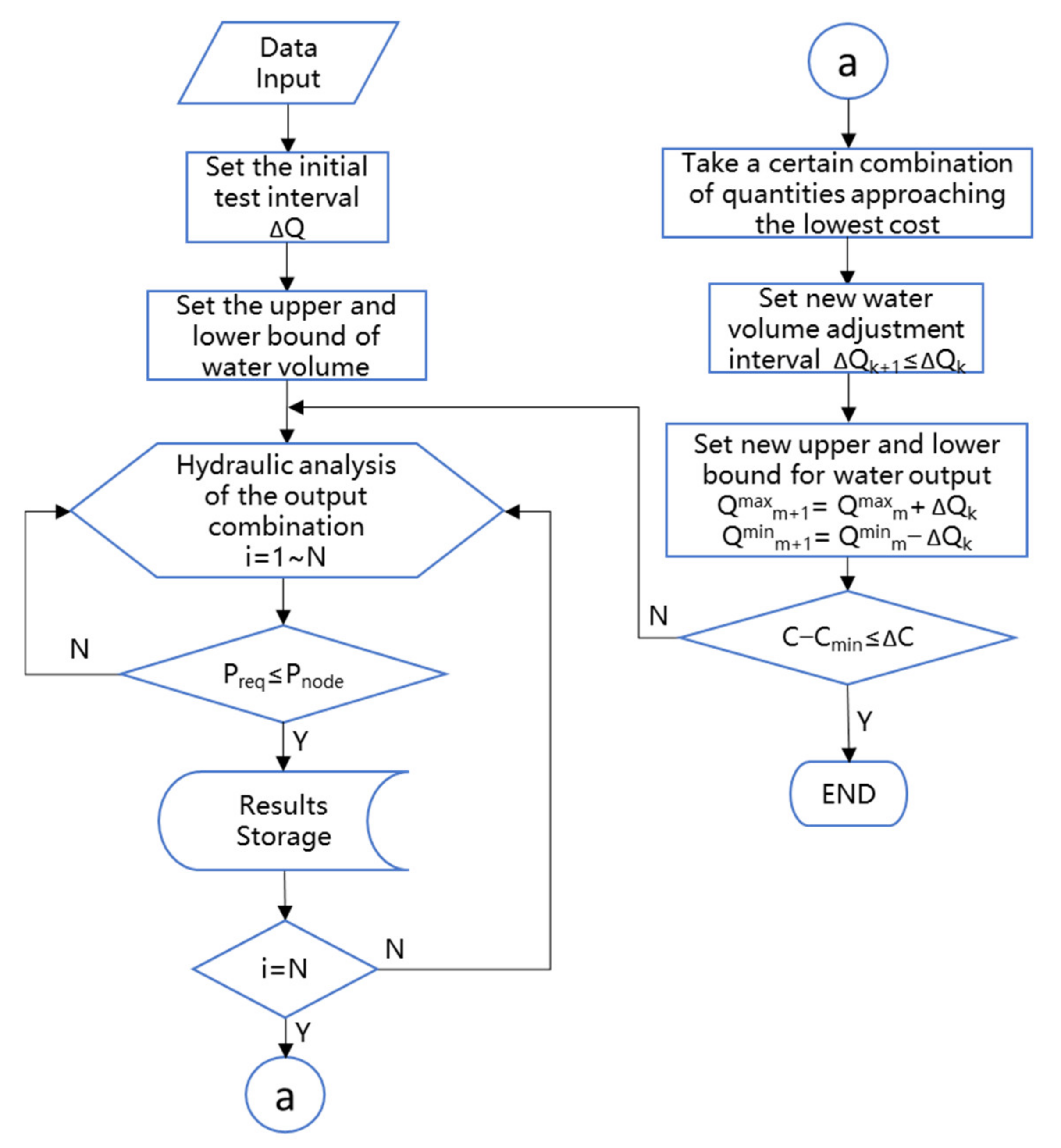
2.3. Uniform Grid Sampling Procedure

To confirm the correctness and efficiency of the aforementioned search method, the uniform grid sampling procedure (UGSP) [31] is adopted for the simple case. All possible combinations of water discharge from each WTP are listed, and the feasible combinations that meet the constraints are filtered out after hydraulic calculations. They are then ranked in order of cost to compare the differences between the two search methods for the optimum solution.

First, we set a reasonable search interval (ΔQ) for the adjustable discharge of the WTP. Then, the water discharge of each WTP is divided into several discrete discharges from 0 to the maximum discharge according to the search interval. Then we arrange and combine the water discharge for all WTPs and carry out the hydraulic calculation for the combination while the total water supply is equal to the total demand. If the constraints of Equations (3) and (4) are met, it means that this combination of water discharge is a feasible solution, and then the combination with the lowest total discharge cost is selected as the optimum operation strategy. To obtain a more accurate discharge operation strategy for a WTP, we can reduce the discharge search interval. Nonetheless, the number of feasible discharge combinations may increase significantly, requiring more calculation time.

In this paper, to avoid missing the optimum solution and to save the computation time of higher precision solutions, we first find all feasible solutions with larger search interval, sort them from the lowest cost to the highest cost, and extract a certain number (or percentage) of lower cost feasible solutions. We then sort out the upper and lower limits of the water discharge from each WTP using the lower limit minus n × ΔQ as the new lower limit and the upper limit plus n × ΔQ as the new upper limit (to avoid missing the optimum solution close to the boundary, n can be taken as 1–2). If the new lower limit is lower than 0, we set it to 0. If the new upper limit is higher than the maximum water discharge, we set it to the maximum water discharge. After that, we set the new search interval as 0.5–0.8 times the original interval, rearrange and combine the water discharge from each WTP, and continue the calculation according to the aforementioned steps until the search accuracy of the water discharge or the minimum cost change is acceptable. The solution is then recognized as the near global optimum. The above calculation process is detailed in Figure 2.

3. Results and Discussions of the Case Study

Firstly, a simple network containing only 4 WTPs, 12 demand nodes and 21 pipelines was tested to apply this search method to an actual system. Next, we analyzed the same network again by UGSP. We compared the results of both methods to understand the characteristics of the optimum solution. Finally, the actual Kaohsiung system in Taiwan was used as a case study to analyze the potential for improvement of the existing operation model, which will serve as a reference for the water company’s allocation of water discharge in the WTP in the future.

This paper used Matlab to write the optimization program and EPANET to perform the hydraulic analysis. The CPU used was i5-8350U and the RAM was 8GB.

3.1. Case 1

3.1.1. Optimization Based on the Concept of Local Search

This case is a WDS for four WTPs. The layout is shown in Figure 3, where there are 12 demand nodes. Each demand node requires 300 cubic meters per day and the elevation is 0 m. The network consists of 21 pipelines. The diameters of the pipelines L1–L17 are 100 mm, and L18–L21 are 200 mm. The lengths of the pipelines in meters are shown in the Figure 3. V1–V4 are flow control valves, which are used to control the water discharge of each WTP. The maximum capacity, head, and cost per unit of water discharge for each WTP are shown in

Table 1. Capacity, head, and unit cost of water discharge from WTP.

Node ID	Design Capacity (m3/day)	Head (m)	Unit Cost (TWD */m3)
R1	1800	30	1.2
R2	1200	20	1.5
R3	1100	20	1
R4	500	15	2

Note: * New Taiwan Dollars.

.

When conducting the hydraulic analysis of the network, the head loss of each pipe is calculated by the Hazen–Williams formula, and the friction coefficient C value of each pipe is assumed to be 100. Assuming that there is no leakage in a single period and the system is supplied by gravity only, the maximum water discharge from each WTP is shown in Table 1, where the minimum water discharge is 0, the maximum head allowed at the demand side is 75 m, and the minimum necessary head is 10 m, i.e., the pressure is 1 kgf/cm². Initially, the flow control valves of all WTPs are fully opened. The results of the hydraulic analysis of the network are shown in Figure 4, and the total cost of the system is shown in

Table 2. Case 1 costs of water discharge in each WTP before optimization.

Plant No.	Daily Delivered Water Volume	Unit Discharge Cost	Total Cost
	m3/day	TWD/m3/day	TWD
R13	1433.2	1.2	1719.84
R14	938.6	1.5	1407.90
R15	891.6	1.0	891.60
R16	336.6	2.0	673.20
Sum	3600.0	-	4692.54

.

Figure 4 shows that the lowest head at the demand side of the network is 13.31 m at N10, which is 10 m higher than the minimum necessary head, so there is space to reduce the discharge head of the WTP, so that the discharge can be changed to reduce the total discharge cost. Then, we applied the optimization method based on the concept of local search to solve the problem, and used the head variation of 1.00 m, 0.50 m, 0.10 m, 0.05 m, and 0.01 m as the search interval of each iteration. The optimized search results are shown in

Table 3. Optimization results of water discharge and total cost for each WTP in Case 1.

Reservoir No.	dh(m)	R1	R2	R3	R4	Sum	Saving Rate	Pmin	Computing Time (sec)	Iterations
Unit discharge cost (TWD/m3/day)	-	1.2	1.5	1.0	2.0	-	-	-	-	-
Water discharge (m3/day)	Not optimized	1433.1	938.6	891.6	336.6	3600.0	-	13.309	-	-
Cost (TWD)		1719.8	1407.9	891.6	673.3	4692.6	0.00%
Water discharge (m3/day)	1.00	1516.6	1004.2	960.7	118.4	3600.0	-	10.881	3	5
Cost (TWD)		1819.9	1506.4	960.7	236.9	4523.9	3.59%
Water discharge (m3/day)	0.50	1527.4	1013.5	970.6	88.5	3600.0	-	10.469	3	10
Cost (TWD)		1832.9	1520.3	970.6	176.9	4500.7	4.09%
Water discharge (m3/day)	0.10	1538.1	1008.1	984.7	69.1	3600.0	-	10.093	3	53
Cost (TWD)		1845.7	1512.1	984.7	138.2	4480.8	4.51%
Water discharge (m3/day)	0.05	1540.0	1002.4	988.6	69.0	3600.0	-	10.043	4	109
Cost (TWD)		1848.1	1503.6	988.6	137.9	4478.2	4.57%
Water discharge (m3/day)	0.01	1540.9	1003.7	989.3	66.1	3600.0	-	10.004	10	545
Cost (TWD)		1849.08	1505.55	989.3	132.2	4476.1	4.61%
Water discharge (m3/day)	1.00–0.002	1541.2	1002.3	990.0	66.6	3600.0	-	10.000	3	33
Cost (TWD)		1849.4	1503.4	990.0	133.1	4475.9	4.62%

.

Table 3 shows that the total cost of water supply for the system before optimization was 4692.6 TWD/day. With the first search interval dh of 1.00 m, the optimization result can save about 3.59% of water supply cost, and with the gradual reduction of the search interval, the savings become larger, and the cost–saving rate gradually converges to 4.61% when the search interval dh is 0.01 m. The results of the hydraulic calculations are shown in Figure 5. When the search interval is reduced from 0.05 m to 0.01 m, the total cost decreases from 4478.2 TWD/day to 4476.1 TWD/day, which is only 2.1 TWD/day and accounts for a tiny percentage of the total cost, which is already acceptable in practice.

Table 3 shows that even with the most considerable calculation quantity being 0.01 m for dh, the calculation time required is only 10 s, indicating that the method is applicable to real-time water supply deployment in this case. The variation of discharge head in each WTP using the dh = 0.01 m iterative search process is shown in Figure 6.

In the initial stage of optimization, the pressure reduction starts from the lowest cost per unit of water discharge in the WTP R4, and in the 475th iteration, the WTP R2 starts to be included in the pressure reduction together with R4 until the lowest head at the node reaches 10.004 m. The search stops, showing that the pressure reduction process of each plant has a monotonically decreasing property.

To improve the computational efficiency, the search interval is dynamically adjusted for iterative calculation. First search with a large search interval until the user’s minimum demand for water pressure is met, then multiply the original search interval by a constant less than 1 (set to 0.5 in this paper) and continue searching until the constraints are met. Repeat the above process until the difference between the minimum nodal pressure and the minimum customer demand is less than an acceptable value (set to 0.001 m in this paper). The results show that not only is the calculation time significantly reduced, but also the residual nodal pressure of the network can be fully utilized, as shown in the last two rows of Table 3.

3.1.2. Uniform Grid Sampling Procedure

The above case was also solved using the UGSP. Firstly, the design capacity of all WTPs was divided into various feasible discharges with a search interval of 100 m³/day. Then the combination of the total discharges of four WTPs equal to the total demand was selected, and the hydraulic simulation was carried out individually to calculate the discharge cost. To simplify the calculation, the feasible solutions were sorted from the lowest cost to the highest cost, and a certain number (or percentage) of the lower cost feasible solutions were extracted. We then summarized the upper and lower limits for the discharges of each WTPs from these feasible solutions and used them as the range for the next search.

In this case, we took all sets smaller than 100 and 100 sets larger than 100. After sampling, we summarized the upper and lower limits of the water discharge from each WTP, and then added and subtracted the original search interval to set the new upper and lower limits of water discharge. We then multiplied the original water discharge search interval of 100 m³/day by 0.5–0.8 as the new water discharge search interval and searched again. We repeated the above steps until the minimum cost improvement was not significant enough and stopped. The results of the search are shown in

Table 4. Uniform grid sampling procedure (UGSP) optimization results.

Search Interval(m3/day)	Upper and Lower Bound of Water Discharge (m3/day)								All Combinations Numbers	Feasible Combinations Numbers	Computing Time(sec)	Least Cost (TWD)	Optimal Water Discharge (m3/day)
ΔQ	R1up	R1lo	R2up	R2lo	R3up	R3lo	R4up	R4lo					QR1	QR2	QR3	QR4
100.0	1800	0	1200	0	1100	0	500	0	17,784	52	2	4550.0	1500	700	1100	300
													1500	900	1000	200
50.0	1600	1000	1200	400	1100	400	500	100	29,835	332	5	4510.0	1550	800	1050	200
													1550	900	1000	150
25.0	1600	1200	1150	450	1100	750	500	100	125,715	1969	14	4485.0	1550	900	1025	125
12.5	1575	1425	1075	600	1100	875	350	50	240,825	3134	25	4478.8	1550	912.5	1025	112.5
7.5	1565	1475	1040	710	1100	935	255	60	363,285	3658	32	4477.3	1542.5	987.5	995	75
5.0	1560	1505	1035	800	1070	965	190	60	342,144	3021	29	4476.5	1545	965	1005	85
2.5	1555	1525	1030	855	1050	970	150	55	1,187,901	6594	74	4476.0	1542.5	990	995	72.5
1.3	1555	1530	1030	895	1035	975	125	55	6,393,177	19,093	397	4476.0	1542.5	990	995	72.5
1.0	1549	1536	1024	935	1018	978	102	56	2,428,020	8833	121	4476.0	1540	1012	986	62

.

Table 4 shows that when the search interval is reduced from 12.5 m³/day to 7.5 m³/day, the cost of water supply is reduced from 4478.8 TWD/day to 4477.3 TWD/day, which is only a 1.5 TWD/day cost reduction and represents a very small percentage of the cost. The calculation could have been stopped, but after observing the combination of water discharge in both cases, it was found that the difference in water discharge from R4 was noticeable. To investigate the optimum solution pattern, the search interval was reduced again, and the calculation continued until the search interval was 1.0 m³/day.

As the search interval gradually decreases, the cost of water supply also becomes lower and lower. When reduced to 2.5 m³/day, the minimum cost of 4476.0 TWD/day is already reached, and even if the interval is further reduced to 1.3 m³/day or 1.0 m³/day, the minimum cost remains the same. However, it can be found that the water discharge combinations from R1 to R4 are slightly different, so it can be speculated that there may be more than one set of near global optimums in this case.

The optimized results with a search interval of 1.0 m³/day are shown in Figure 7.

When using the UGSP, the minimum cost is only 0.1 TWD/day different from that of the optimization method based on the concept of local search. The water discharge of each WTP is also similar. The calculation time for the UGSP is 181 s to reach the minimum cost of 4476.0 TWD/day with a search interval of at least 2.5 m³/day without setting new search intervals and upper and lower limits manually. If we adopt the optimization based on the concept of neighbor search, it only takes 10 s, which is a significant advantage in optimization efficiency.

3.2. Case 2 (Adopt Optimization Based on the Concept of Local Search Only)

This example focuses on the practical water supply system scheduling strategies during off-peak, normal, and peak periods. The model was simulated with reference to the water supply system in Kaohsiung, Taiwan. The model has 6 WTPs, 117 nodes, and 150 pipelines with diameters ranging from 500 mm to 3200 mm. To simplify the calculation, pipes with diameters less than 500 mm are ignored. 18 valves are set up in the model according to the current situation. The check valve (CV) is located at the outlet of the WTP to prevent backflow. The flow control valve (FCV) is located downstream of the check valve and sets the maximum flow as the design capacity of the plant. The pressure breaker valve (PBV) is located downstream of the FCV to control the discharge head of the WTP. The layout of the network is shown in Figure 8.

The total water consumption of the system is 1.28 million m³/day for domestic use. By taking an hour as the minimum period for analysis, the total water consumption of the system in each hour of the day is shown in the Figure 9.

The off-peak period runs from 01:00–04:00, and its water consumption Q_min is 42,250 m³/hr. The normal period runs from 07:00–16:00, and its water consumption Q_ave is 55,292 m³/hr. The peak period runs from 18:00–20:00, and its water consumption Q_max is 63,167 m³/hr. In practice, each WTP uses the water stored in the tank to increase the water discharge during peak periods and uses the off-peak periods to refill the tank. From Figure 9, we can estimate that the maximum water discharge during the peak and off-peak periods is close to the design capacity plus and minus 20%, as shown in

Table 5. Maximum water discharge during off-peak, normal, and peak periods for each WTP.

(m3/Hr)	QR1max	QR2max	QR3max	QR4max	QR5max	QR6max
off-peak	3333	21,667	15,000	1200	7500	10,000
normal	4167	27,083	18,750	1500	9375	12,500
peak	5000	32,500	22,500	1800	11,250	15,000

.

The WTPs R1, R2, and R6 deliver water to the customer by gravity. The total head of each WTP is 82 m, 70 m, and 50 m respectively. The cost function for these includes the source cost and the treatment cost. The WTPs R3, R4, and R5 deliver water to the customer by pump. The total head of each WTP is 48 m, 71 m, and 66.9 m respectively. The cost function of these includes the source cost, the treatment cost, and the pumping cost. The estimated pumping cost functions of WTPs R3, R4, and R5, according to the process described in Section 2.1, are shown in Figure 10, Figure 11 and Figure 12.

Figure 10, Figure 11 and Figure 12 show a linear regression to obtain the pumping cost function based on the hourly electricity consumption and hourly water discharge of WTPs R3–R5. The coefficient of determination is between 0.8 and 0.9, which indicates that the fitting function can achieve a reasonable prediction. Based on these records and the fitting function, we can see that the relationship between the unit cost per volume and the water discharge. It means that the higher the water discharge, the lower the unit cost per volume. It is reasonable to recognize that when the WTP was designed, the design capacity was used to plan the configuration of pumping units for maximum energy efficiency, including specifications and quantities. However, during the operation period, the water discharge is often lower than the design capacity, and the energy efficiency is lower.

Referring to the water company’s annual operating reports and combining the above pumping costs, the cost functions for each WTP can be obtained, as shown in

Table 6. Design capacity, head, and unit cost of water discharge for each WTP(TWD/m³).

	R1	R2	R3	R4	R5	R6
water source costs	1.401	0.184	0.484	0.223	0.215	0.639
treatment costs	1.274	0.461	2.127	2.247	2.128	1.485
pumping costs	0	0	CR3pump (QR3)	CR4pump (QR4)	CR5pump (QR5)	0
sum	2.675	0.645	2.611 + CR3pump (QR3)	2.470 + CR4pump (QR4)	2.342 + CR5pump (QR5)	2.124

.

Table 6 shows that the total unit cost per volume for WTPs R1, R2, and R6 is a certain value. The total unit cost per volume for WTPs R3–R5 is a certain value plus a variable value. The variable value can be obtained by substituting the WTP’s water discharge into the fitting function.

We set the head reduction of eight PBVs alternatively as a search variable. Its initial setting value was 0, i.e., no pressure reduction. After that, a local search was conducted for all PBVs, the optimization results of which are shown in

Table 7. Optimized water discharge for off-peak, normal, and peak periods at each WTP.

(m3/Hr)	QR1	QR2	QR3	QR4	QR5	QR6	Total Cost (TWD)	Savings Ratio
off-peak	3473.0	20,146.0	9987.5	885.9	4266.4	3491.3	77,590
off-peak (optimized)	3333.3 *	21,416.7	0.0	0.0	7500.0 *	10,000.0 *	65,489	15.6%
normal	3740.8	20,579.9	14,983.9	1260.2	6051.1	8675.8	109,588
normal (optimized)	4166.7 *	23,004.2	14,120.8	1500.0 *	0.0	12,500.0 *	99,764	9.0%
peak	3690.1	20,665.1	20,059.8	1282.3	8114.0	9355.3	130,032
peak (optimized)	5000.0 *	24,234.9	7681.7	0.0	11,250.0 *	15,000.0 *	113,489	12.7%

* indicates the maximum water discharge.

.

As shown in Table 7, the optimized results during off-peak, normal, and peak periods can save 15.6%, 9.0%, and 12.7% of water supply costs, respectively, compared to the pre-optimization period.

The optimization results in Table 7 can provide managers with information to make decisions about the water delivery from each WTP. The WTPs R1 and R6 supply water using gravity and are located at the northern and southern ends of the WDS respectively. The optimized result is that both sites are discharged at the upper limit in all three periods. This means that these two sites play an important role in stabilizing WDS water supply and reducing costs. Future expansions can be evaluated to increase the design capacity. The WTP R2 also supplies water using gravity. The optimized result relating to this WTP is that the water discharge is higher in all three periods than before optimization, so water discharge can be increased appropriately in normal operation. The WTP R3 supplies water using pumps. The optimized result in this case is that the water discharge is lower in all three periods than before optimization, which shows that this site has a negative impact on the stabilization of WDS water supply and cost reduction. Thus, water discharge can be reduced appropriately during normal operation. The WTPs R4 and R5 also supply water using pumps. The related optimized result is that the water discharge varies greatly from zero to the upper limit in all three periods, and it can be found that the water is discharged at the upper limit in one site when the water is discharged at zero in the other site. The two WTPs complement each other in stabilizing the WDS water supply and reducing costs.

4. Conclusions

This study investigates the real-time operation of multiple WTPs. The research proposition was to provide the required water volume and head for the WDS with minimum operational cost. The objective in practice was to minimize total the operating costs of all WTPs. The decision variables were the water discharges or heads provided by the WTPs. The constraints were the capacity of every WTP and the head requirements for the customers in the WDS.

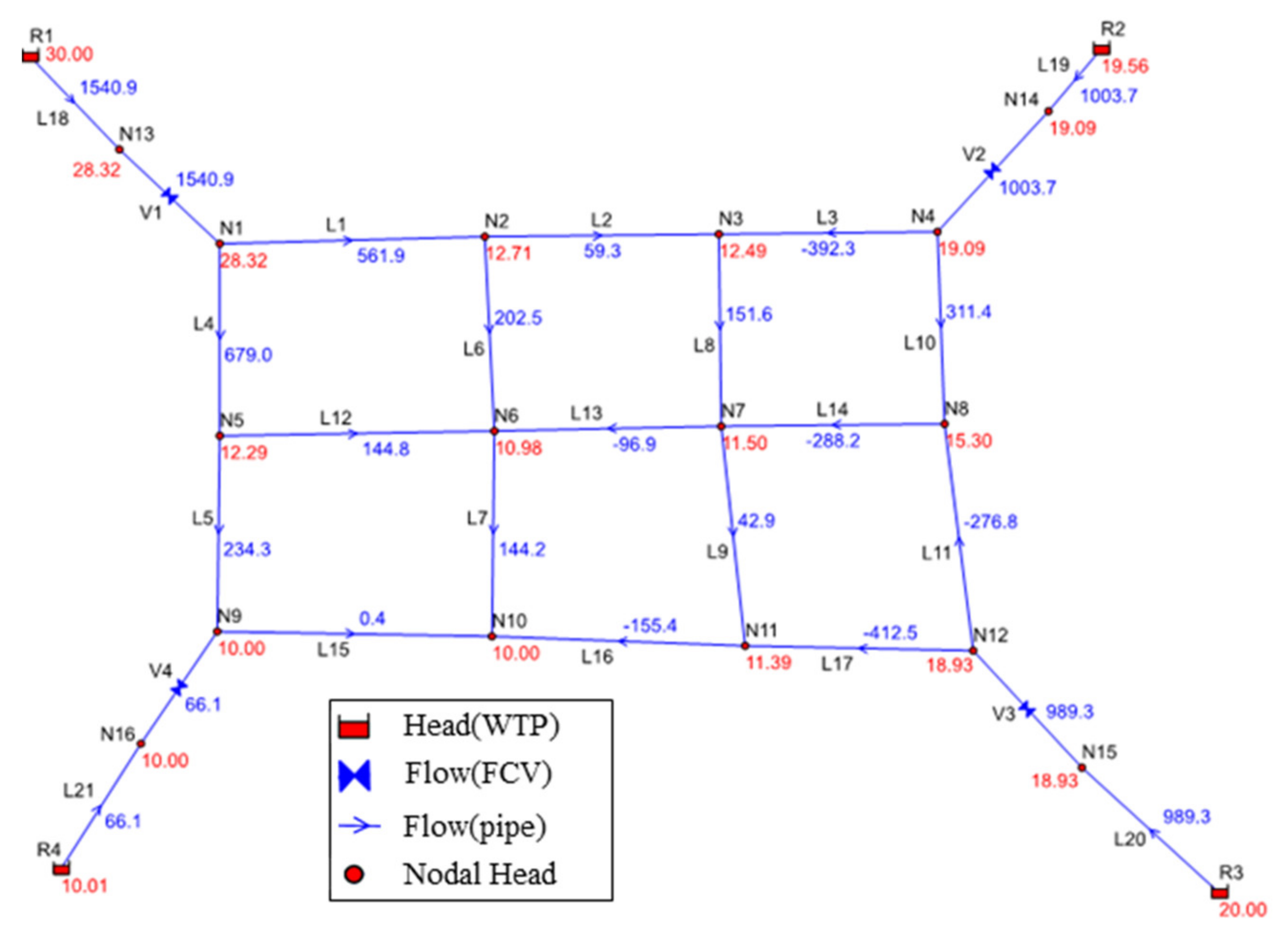
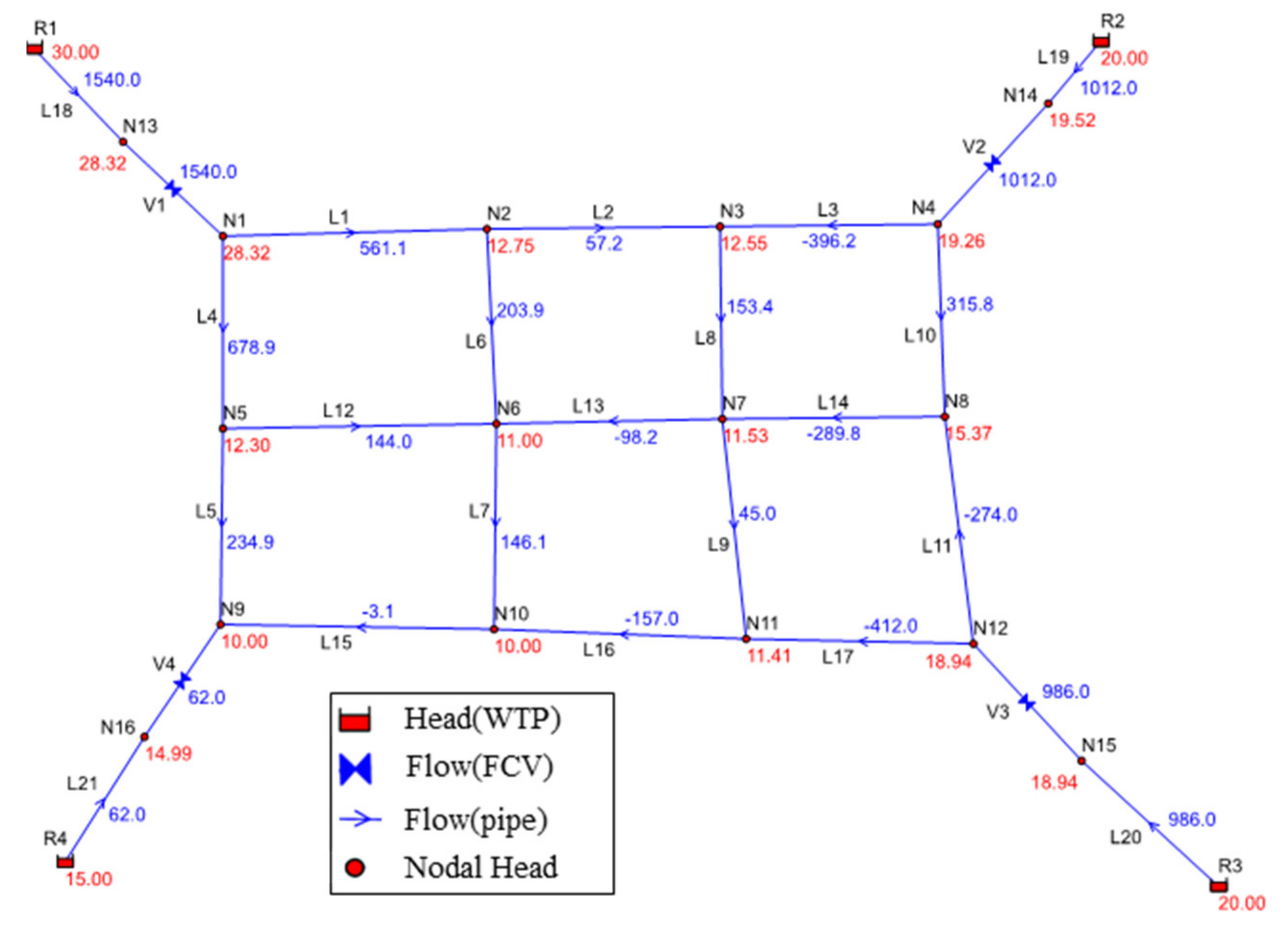
Applying the optimization method based on the local search concept proposed in this paper to a hypothetical water supply system containing four WTPs with different unit discharge costs (Case 1), we obtained a minimum cost of optimization of 4476.1 TWD/day, which is only 0.1 TWD/day higher than the result obtained by using the UGSP method. We also obtained the same saving rate of discharge cost, at about 4.6%, and the discharge of each WTP was similar. In this case, the optimum solution obtained using the optimization based on the concept of local search was almost the same as the near global optimum obtained by the UGSP, but the advantage of the optimization based on the local search concept was very obvious in terms of the computational time consumed.

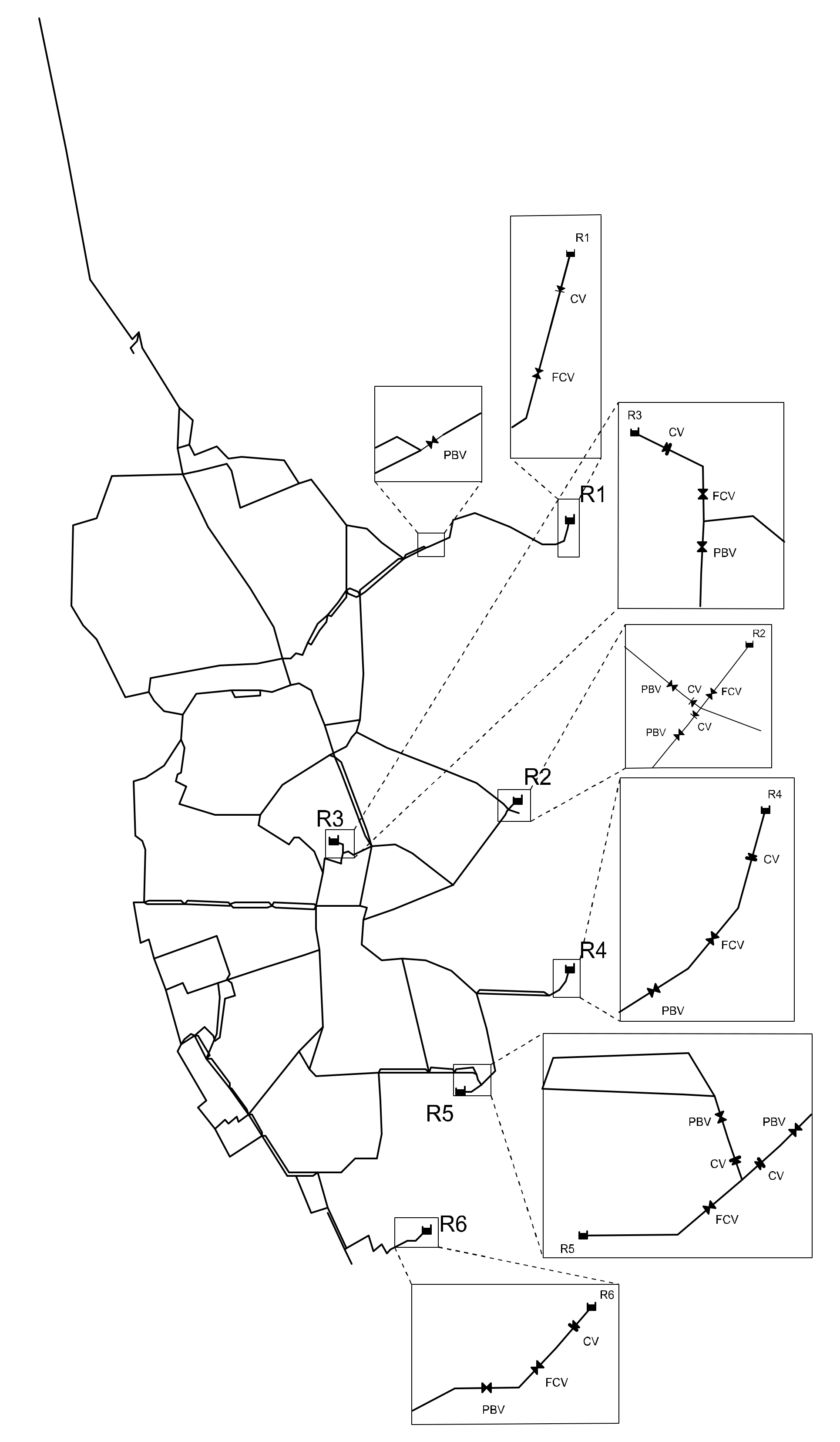
In Case 2, EPANET was used to build a simulated Kaohsiung system in Taiwan with six WTPs, and various special function valves were set up near the WTP outlet according to the actual situation. These included the flow direction being controlled by a check valve (CV), the flow being controlled by a flow control valve (FCV), and the pressure at the downstream of the pipeline being controlled by a pressure breaker valve (PBV). The constraints could be automatically met by using EPANET’s built-in hydraulic analysis function during optimization. The optimization results showed that the total cost of water supply was 15.6%, 9.0%, and 12.7% lower during off-peak, normal, and peak periods, respectively, when compared to before the optimization.

By dynamically adjusting the search interval, not only did the calculation efficiency improved significantly, but also the residual nodal pressure of the network was fully utilized. It was also possible to avoid falling into the local optimum solution and to obtain a near global optimum solution.

According to the optimization proposed in this paper, it is possible to observe the iterative search results and find that in the neighboring water supply area, reducing the discharge pressure of the WTP with a higher unit discharge cost will reduce the discharge. At the same time, the discharge of the WTP with a lower unit discharge cost will increase, which will lead to the reduction of the total system water supply cost. When the water discharge from the low-cost WTP reaches the upper limit, the hydraulic balance of the system will change. The low-cost plant will continue to maintain the upper limit of water discharge, while other higher-cost plants will continue to search for the most prominent economic savings per minimum head change, until the minimum head at the node meets the necessary head.

The optimized search method developed in this paper is simple in principle and can be easily modeled using the commonly used hydraulic analysis software EPANET. Various constraints can be automatically satisfied by building different functional valve categories. Even with a complex system of up to 6 WTPs, 117 nodes, and 150 pipelines, an acceptable and reasonable solution can be found in a short time. For a management company, this method can not only provide an immediate operational reference for different water consumption periods during peak and off-peak periods, but it can also facilitate the continued use of the company’s internal annual cost and water discharge data to analyze the potential improvement of the existing operation model and further develop the outsourcing operation strategy of the WTP.