Article

Harmonizing and Extending Fragmented 100 Year Flood Hazard Maps in Canada’s Capital Region Using Random Forest Classification

by
Shelina A. Bhuiyan
1,*,
Clement P. Bataille
1,2,† and
Heather McGrath
3,†
1
Department of Earth and Environmental Sciences, University of Ottawa, 120 University, Ottawa, ON K1N 6N5, Canada
2
Department of Biology, University of Ottawa, 120 University, Ottawa, ON K1N 6N5, Canada
3
Natural Resources Canada, Ottawa, ON K1A 0Y7, Canada
*
Author to whom correspondence should be addressed.
Co Supervisor.
Water 2022, 14(23), 3801; https://doi.org/10.3390/w14233801
Submission received: 4 September 2022 / Revised: 29 October 2022 / Accepted: 20 November 2022 / Published: 22 November 2022

Abstract

:
With the record breaking flood experienced in Canada’s capital region in 2017 and 2019, there is an urgent need to update and harmonize existing flood hazard maps and fill in the spatial gaps between them to improve flood mitigation strategies. To achieve this goal, we aim to develop a novel approach using machine learning classification (i.e., random forest). We used existing fragmented flood hazard maps along the Ottawa River to train a random forest classification model using a range of flood conditioning factors. We then applied this classification across the Capital Region to fill in the spatial gaps between existing flood hazard maps and generate a harmonized high-resolution (1 m) 100 year flood susceptibility map. When validated against recently produced 100 year flood hazard maps across the capital region, we find that this random forest classification approach yields a highly accurate flood susceptibility map. We argue that the machine learning classification approach is a promising technique to fill in the spatial gaps between existing flood hazard maps and create harmonized high-resolution flood susceptibility maps across flood-vulnerable areas. However, caution must be taken in selecting suitable flood conditioning factors and extrapolating classification to areas with similar characteristics to the training sites. The resulted harmonized and spatially continuous flood susceptibility map has wide-reaching relevance for flood mitigation planning in the capital region. The machine learning approach and flood classification optimization method developed in this study is also a first step toward Natural Resources Canada’s aim of creating a spatially continuous flood susceptibility map across the Ottawa River watershed. Our modeling approach is transferable to harmonize flood maps and fill in spatial gaps in other regions of the world and will help mitigate flood disasters by providing accurate flood data for urban planning.

1. Introduction

With urbanization and climate change, the world is experiencing an increase in costly and destructive flooding events [1]. Floods threaten human societies, infrastructures, natural ecosystems and wildlife. Floods can also transport and mobilize environmentally persistent pollutants including metals stored in alluvial sediments and cause severe water pollution [2]. In Canada, flood is the costliest natural hazard [3] and with Canada’s accelerated warming, it is predicted that more frequent and intense floods will occur in the next decades [4,5]. Since 1948, the provinces of Ontario and Quebec have experienced an increase in winter precipitation accompanied by a warmer and wetter spring [4]. These factors have likely contributed to the record breaking spring flood event in 2017 and 2019 across the Ottawa River watershed [6,7]. These flood events occurred in spite of the Ottawa River’s integrated river discharge control system, including 50 major dams and 13 principal reservoirs [8,9]. These record breaking floods have caused significant socioeconomic, ecotoxicological and ecosystem damage, particularly in the capital region [10]. Consequently, it is critical to identify flood susceptible areas, defined as the potential flood zones in the watershed [11]. Harmonized and spatially continuous flood hazard maps are key tools to enhance the resilience and sustainability of infrastructures and ecosystems by adapting land use plans, and improving emergency response and flood mitigation risks planning [12].
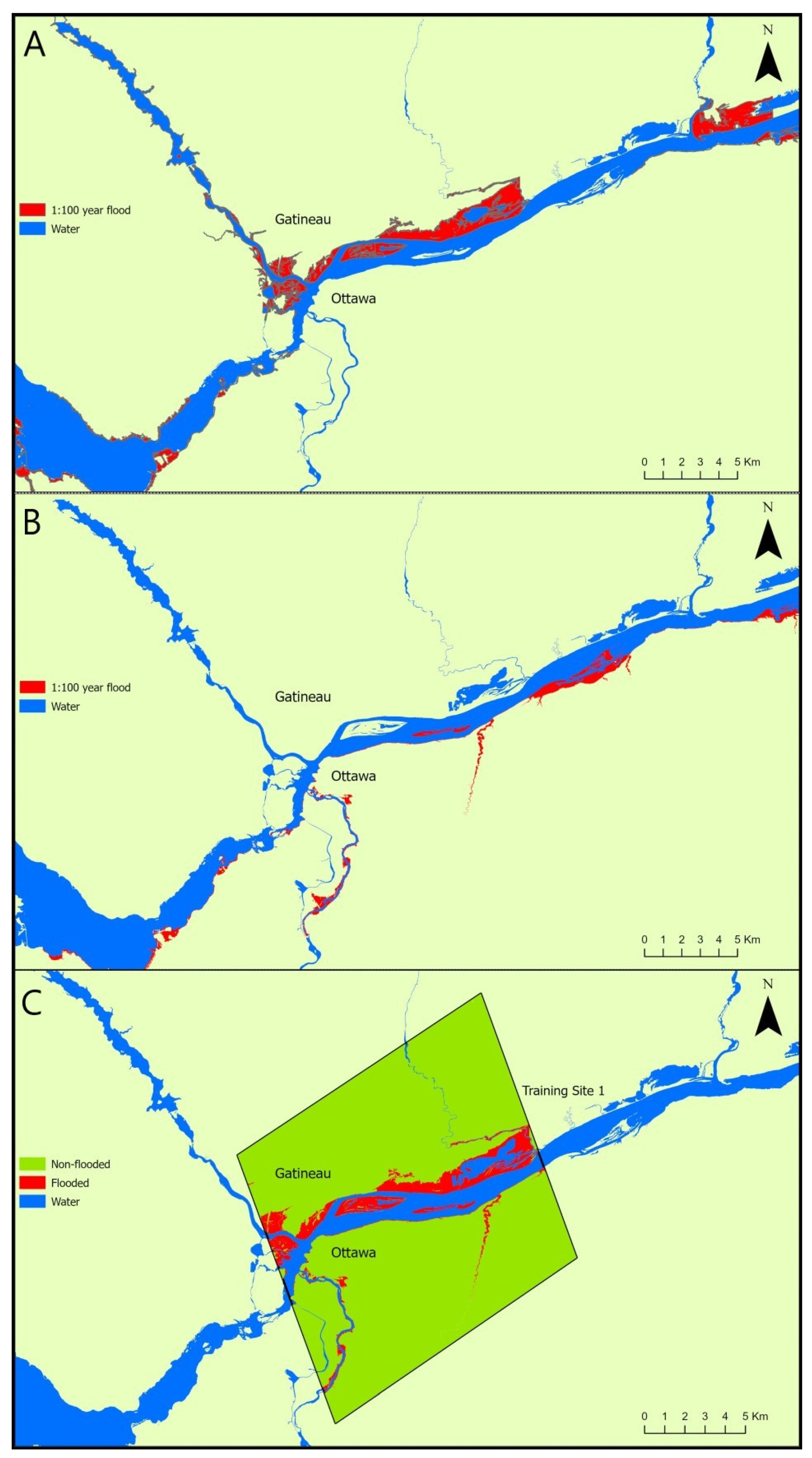
However, since flood hazard mapping is completed at the provincial level and is often conducted by different municipalities at different times and by different companies, there is a lack of consistency between flood hazard maps. This is particularly true for the Ottawa River watershed, where the Ottawa River serves as a natural border between Quebec and Ontario (Figure 1) for hundreds of kilometers. For example, around the capital region, many existing flood hazard maps, generated during the Flood Damage Reduction Program (FDRP), show discontinuity along the Ottawa River shoreline and between the two provinces (Figure 2A). These fragmented maps are also largely outdated with many being created or last updated in the 1980s. These spatial gaps, inconsistencies and lack of standardization between the provinces are making flood mitigation planning more challenging. In this context, there is an urgent need to develop an approach to harmonize and update the existing flood hazard maps and generate a spatially continuous map across the watershed so that localities can best prepare flood mitigation plans.
Municipalities mostly use hydrologic-hydraulic-based models (i.e., engineering models) to generate 100 year flood hazard maps, defined as the probability of an area to be flooded once in a 100 year return period [12]. Hydrologic analyses are focused on quantifying the volumetric flow rate of water (i.e., using rainfall and evaporation data) to determine peak flood discharges and flood occurrence frequencies [13,14,15]. Hydraulic analyses are focused on flow scenarios (e.g., depth of flow, flow velocity, and forces) in streams and infrastructure to estimate the water surface elevations and behaviour for a selected return period (e.g., 100 year flood) [13,14,15]. These 100 year flood hazard maps are the basis for land use planning and for regulating future development in an effort to mitigate flood risks. Although these engineering models achieve a high level of accuracy (using calibration data), they are, however, very costly and require extensive fieldwork and data collection [16,17]. Therefore, these models are run in a spatially discontinuous manner, prioritizing populated localities and using a standard provincially regulated flood return period (e.g., 100 year return period in Ontario and Quebec). Considering the limitations of the existing hydrologic-hydraulic models and in a context of rapid climate change and increasing flood damages, Natural Resources Canada (NRCan) is exploring approaches to update, harmonize and extend the coverage of existing flood hazard maps to create a spatially continuous flood susceptibility map across the Ottawa River watershed. This pilot study aims to explore the potential of machine learning classification, more specifically random forest, to fill in the spatial gaps and harmonize the existing flood hazard maps of the Ottawa River in the Capital region.
Machine learning classification using a range of flood conditioning factors has shown promises to delineate more accurate flood susceptibility maps [16,17,18,19,20,21,22]. The flood conditioning factors are generally related to topography (e.g., elevation, aspect and distance to river), hydrology (e.g., precipitation), and geology (e.g., land cover, soil type and soil drainage capacity) [23]. However, the selection of suitable flood conditioning factors vary depending on the study area [24]. For example, soil drainage capacity and impervious surfaces will determine the rate and amount of surface runoff generation [11,25], and might, therefore, play a more important role in urban areas. Therefore, selecting the most relevant flood conditioning factors is the most crucial step in machine learning classification applied to flood mapping [11,22]. The hypothesis proposed here is that using machine learning classification (i.e., random forest) and a series of flood conditioning factors, we will be able to generate an accurate, harmonized and spatially continuous 100 year flood susceptibility map around the capital region of Canada.

2. Materials and Methods

2.1. Study Area

The Ottawa River is the second largest river in eastern Canada (1271 km) and acts as a boundary separating the provinces of Ontario and Quebec [26,27]. Its watershed covers an area of over 140,000 km2 with 65% on the Quebec side and 35% on the Ontario side [26,27]. Our study area focuses on the central area of the National Capital Region of Ottawa–Gatineau, which consists of the Canadian capital of Ottawa, Ontario and the neighboring city of Gatineau, Quebec (Figure 1). The selected study area covers an area of 1972.62 km2 covering approximately 93 km length of the Ottawa River. Our goal is to train a random forest classification model using existing fragmented flood hazard maps, then apply the model to the entire study area to generate an updated, harmonized and continuous flood susceptibility map.

2.2. Random Forest Classification

Machine learning (ML) classification has shown promise in generating flood susceptible areas in different regions across the globe using a range of flood conditioning factors [11,17,20,22,28]. There are a variety of ML algorithms but random forest is one of the most popular ones in flood susceptibility mapping studies [16,20,21,29,30]. A study testing 179 classification algorithms has shown random forest classification to be the most accurate classification approach for these types of studies [31].
Random forest is an ensemble learning approach that is based on generating an ensemble of decision trees [18]. Random forest uses an ensemble technique known as Bagging (also known as Bootstrap aggregation) to randomly sample from the original data set resulting in n number of data subsets (i.e., bootstrapped samples) to train an ensemble of decision trees. Each decision tree is trained using a random subset of predictors (i.e., flood conditioning factors) [32]. The term “random” is from the random selection of bootstrapped samples and a random selection of predictors when training each decision tree. The term “forest” is from the ensemble of decision trees that are created [32]. This ensemble of decision trees are then used in the classification of flood by running input data through the decision trees and taking the classifier with the majority of votes as the resulting flood prediction [32]. An error rate is calculated using a data subset that were not used in the bootstrapped samples, named as out of bag or OOB data. The OOB data are tested against the decision trees to evaluate correct predictions. The prediction results for the OOB are aggregated and used to calculate the error rate [32].
Random forest classification of flood susceptibility requires two types of input data: (1) a series of potential geospatial predictors of flood, commonly known as flood conditioning factors, and (2) a training set of points and a testing set of points derived from existing flood hazard maps with their respective flood class (flooded and non-flooded).

2.3. Existing Flood Hazard Maps Used for Training Random Forest Classification

In this study, we first compiled existing flood hazard maps from different sources. NRCan provided existing historical FDRP maps, which contain discontinuous flood hazard maps along the Ottawa River (red patches in Figure 2A). The FDRP maps were created as part of a national program (1976–1996) with funding from both the federal and provincial governments covering 900 communities [13,33]. They were created using traditional engineering hydrologic-hydraulic methods and based on data available at the time, such as topographic maps, which were less precise than today [34]. Within our study area, FDRP maps have a larger coverage on the Quebec side as opposed to the Ontario side (Figure 2A).
To train a model across provincial boundaries, we need to sample an area with continuous flood hazard maps from both sides of the Ottawa River. We aimed for a more balanced distribution of training points between the Ontario side and Quebec side of the river. The FDRP maps lacked continuity on the Ontario side of our study area (Figure 2A). Therefore, we obtained a flood hazard map from the RVCA (Rideau Valley Conservation Authority, 2014) [35] to cover the Ontario side (Figure 1B). The RVCA map for the Ottawa River was created to replace the 30 year old flood hazard maps (created as part of the FDRP). This map on the Ontario side was generated using more modern hydrologic-hydraulic methods and high quality and high-resolution LiDAR data. This map was generated following the technical guidelines by FDRP [34].
We combined these flood hazard maps, using the FDRP map for the Quebec side and the RCVA map for the Ontario side of the Ottawa River (Figure 2C). These combined flood hazard maps provide a continuous floodplain from downtown Ottawa–Gatineau toward the east for ~15.4 km along the Ottawa River. We selected this 15.4 km section to create our initial training area (covering 197.56 km2 named as training site 1, Figure 2C) as it provides the largest continuous flood maps on both sides of the river. The selected training site 1 covers the most populated and urbanized areas in the capital region along the Ottawa River, which were severely impacted by the recent floods.

2.4. Flood Conditioning Factors as Predictors of Flood

Various factors contribute to determining which zones are likely to be flooded. To generate a flood susceptibility map using random forest classification, we compiled a series of geospatial flood conditioning factors that are likely to influence flood occurrences based on the literature and availability of high-resolution geospatial data. We compiled a total of 14 potential flood conditioning factors as predictors of flood. All the 14 flood conditioning factors, their resolution and sources, are listed on Table 1 and shown in Figures S1 and S2.
We used high resolution (1 m) elevation data and various elevation derivatives since they play an important role in determining flood prone areas [16,36]. First, the 1 m resolution elevation dataset of Quebec and Ontario were merged and a spatial gap between the two provinces representing the Ottawa River was filled using the focal statistics tool in ArcGIS Pro. We then derived the slope, aspect, curvature, roughness, topographic roughness index (TRI), topographic position index (TPI), and stream power index (SPI) from the 1 m resolution elevation raster. Slope, aspect and curvature were calculated using spatial analyst tools in ArcGIS Pro. Roughness, TRI and TPI were calculated using the raster package in R [37]. SPI was calculated using the whitebox package in R [38].
Elevation and slope are critical in flood prediction as low elevation and flat areas with gentle slopes are particularly susceptible to river flooding [11,23,24]. Aspect (orientation of slope) is another important flood conditioning factor as it influences the micro-climate (i.e., precipitation amount and temperature) [11,23]. We use curvature (classified as flat, convex or concave) as it accounts for flatness in the region and naturally flat areas are prone to flooding as water flows downhill to flat areas [16,23]. Roughness elements (e.g., surface irregularities) play an important role in the hydrology of a floodplain, therefore roughness and TRI are used as important flood conditioning factors to express elevation differences between adjacent cells of a DEM [11]. Roughness is defined as the difference between the maximum and the minimum value of a cell and its 8 surrounding cells, and TRI is defined as the mean of the absolute differences between the value of a cell and the value of its 8 surrounding cells [37]. TPI is another important terrain classification method where the positive index represent hills and ridges and the negative index represents sunken features such as valleys [39]. TPI is defined as the difference between the value of a cell and the mean value of its 8 surrounding cells [37]. SPI measures potential streams erosion caused by surface runoff and, therefore, indicates the stability of an area and can play a role in flood prediction [11,16]. For example, an increase in the catchment area and slope gradient increases the runoff accumulated from the upslope areas as well as the velocity of the runoff, thereby contributing to erosion risks [40].
TWI (topographic wetness index) is a widespread hydrological analysis and defined as the potential water accumulation at a location based on cumulative upslopes and the tendency of gravitational forces [11,16]. For example, areas that are prone to water accumulation or flood are represented by high TWI values whereas well-drained dry areas are represented by low TWI values [41]. Since at 1 m resolution TWI is not very meaningful and a minimum of 30 m resolution is recommended [42], we used a 30 m resolution elevation dataset to derive the TWI using the dynatopmodel package in R [42].
HAR (or height above river) is a normalized DEM providing the relative elevation above a river (i.e., Ottawa River). HAND (or height above nearest drainage network), its counterpart representing the relative height above the nearest stream, has recently been used in several flood studies in Canada [16,29]. In this study, we have opted for HAR as our study focuses on a smaller scale and flooding from the main river (i.e., Ottawa River). In addition, HAR is better suited for LiDAR based high resolution DEM [43]. HAR with respect to the Ottawa River was calculated from the 1 m elevation raster and the National Hydrographic Network (NHN, representing the Ottawa River). HAR values are generated at each location by subtracting a calculated weighted average river elevation from the elevation of individual grid cells [44]. Since there was minimal variation of elevation in the neighboring river cells at 1 m resolution, we used the original elevation for the river cells instead of the weight average. The elevation data of the river was extracted to create the elevation raster of the Ottawa River. For all land cells the elevation of the nearest river cell (i.e., the river cell closest to land) was derived using the Euclidean allocation tool in ArcGIS Pro. Then, the nearest river elevation value was subtracted from the land elevation value to derive the HAR values at each location.
Distance to river is one of the most important flood conditioning factors as river flooding occurs along the river and streams affecting the areas closest to the river bank [11,23]. The distance to river was calculated from the NHN (representing the Ottawa River) using the Euclidean distance tool in ArcGIS Pro. Urban flooding is influenced by road networks and built surroundings as they contribute to imperviousness (decreased infiltration capacity) resulting in large and quick runoff [11,23]. We used the road network obtained from the City of Ottawa and City of Gatineau. Distance to road was calculated using the Euclidean distance tool in ArcGIS Pro. Lastly, the land cover and surface geology were obtained from Natural Resources Canada. Surficial geology controls water movement through channels and defines active fluvial systems [30], therefore influences flood peak discharges and volumes particularly for large basins [45]. Land cover or land use influences the water flow components, such as infiltration, evapotranspiration and run-off generation through the natural and built environment [11]; for example, forest cover contributes to water retention through natural processes (e.g., transpiration and infiltration into the soil) and, in contrast, urbanization contributes to imperviousness and runoff generation [30].
All the geospatial data were projected to NAD1983 MTM zone 9 with a 1 m resolution. The vector data surface geology was converted to raster and the coarse resolution datasets (TWI, land cover and surface geology) were resampled to 1 m resolution to align with the other 1 m resolution flood conditioning factors.
Table 1. Flood conditioning factors and their resolution and sources.
Flood Conditioning FactorsResolutionReferences
(1)
Elevation
1 mCity of Ottawa for the Ontario side [46] and the Ministry of Forest Wildlife and Parks [47] for the Quebec side
(2)
Height above river (HAR)
1 mderived from 1 m resolution elevation [46,47] and National Hydrographic Network (NHN) [44]
(3)
Slope
1 mderived from 1 m resolution elevation [46,47]
(4)
Aspect
1 mderived from 1 m resolution elevation [46,47]
(5)
Curvature
1 mderived from 1 m resolution elevation [46,47]
(6)
Roughness
1 mderived from 1 m resolution elevation [46,47]
(7)
Topographic roughness index (TRI)
1 mderived from 1 m resolution elevation [46,47]
(8)
Topographic position index (TPI)
1 mderived from 1 m resolution elevation [46,47]
(9)
Stream power index (SPI)
1 mderived from 1 m resolution elevation [46,47]
(10)
Topographic wetness index (TWI)
30 mderived from a 30 m resolution elevation dataset obtained from the Open Government Portal [48]
(11)
Distance to river
1 mcalculated using the National Hydrological Network (NHN) [49].
(12)
Distance to road
1 mcalculated based on the road network obtained from the City of Ottawa and City of Gatineau [50,51].
(13)
Land cover
30 mNatural Resources Canada [52]
(14)
Surface geology
25 mNatural Resources Canada [53]

2.5. Training and Testing Data for the Random Forest Classification

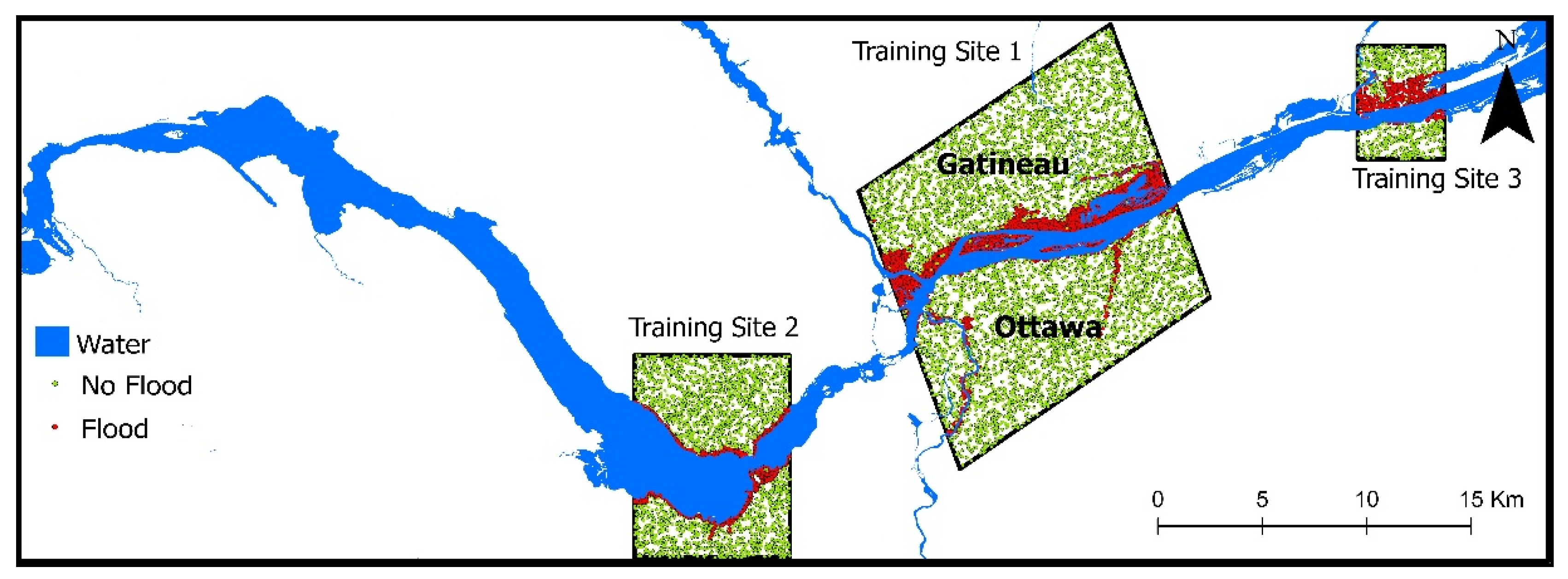
To derive training and testing data, we used the FDRP and RVCA maps and defined the flood classes. The “flooded” class was defined as the land within the existing flood hazard areas and the “non-flooded” class was defined as the land area beyond the existing flood hazard areas (Figure 2C). A total of 10,000 samples (5000 for the “flooded” class and 5000 for the “non-flooded” class) were generated using the Create Random Points tool in ArcGIS Pro within the training site 1 (Figure 3). Values for each flood conditioning factor were extracted at the location of each sample point using the Extract Multi Values to Points tool in ArcGIS Pro. The resulting matrix contained the dependent factor (with “flooded” or “non-flooded” classes) and 14 flood conditioning factors for all 10,000 sample points. We used this matrix to train a random forest classification using the caret (Classification and Regression Training) package in R [54].
The 10,000 sample points were then divided into a set of training points (70%, 7000 sample points) and a set of testing points (30%, 3000 sample points) randomly in R. This 70:30 ratio for training and testing is commonly found in the literature [16,23]. We tested the model’s performance, using between 1000 and 30,000 sample points. Increasing the sample points beyond 10,000 did not significantly improve the accuracy of the classification. Therefore, we ultimately chose 10,000 sample points (training and testing points) to run the random forest classification.

2.6. Selecting Optimal Set of Flood Conditioning Factors and Single Site Training and Extrapolation

We used the VSURF package (Variable Selecting Using Random Forest), to determine the most optimal set of flood conditioning factors for the classification of flooded and non-flooded classes [55]. VSURF combines the most important flood conditioning factors by determining the importance of each of the flood conditioning factors and removing the redundant flood conditioning factors.
With the selected combination of flood conditioning factors, we trained the random forest classification model using the training subset (70% of the sample points). The caret package and the ranger classification method, a fast implementation of random forest for high dimensional data were used for training this model in R [54,56]. The train function tests different parameters (e.g., mtry, split rule and minimum node size) and determines the optimized setting to obtain a final model with the highest accuracy.
To further optimize the model, we used the k-fold cross-validation feature in the caret package. We then validated the single site trained model against the testing subset (30% of the sample points). Then, using this single site trained model, we extrapolated the flood prediction across our study area to fill in the spatial gaps and generate a harmonized flood susceptibility map across the Capital region.
We validated our flood susceptibility map against recently developed NFHDL maps (National Flood Hazard Data Layer, newer and more spatially continuous flood hazard maps available in the Ottawa River watershed) provided by NRCan. The NFHDL maps are a compilation of all the flood hazard maps developed by the provinces and territories across Canada. Although it does contain some FDRP flood maps, most of the contents are newer maps, generated between the mid-1990s and 2021. The provinces and territories have shared these maps with the federal government so that the federal government have a better understanding of the age and coverage of the existing flood hazard maps across the country.

2.7. Multi-Sites Training and Extrapolation: Extending Training and Testing Data to Improve Extrapolation

To optimize the classification model and extrapolation (single site training in Section 2.6), we selected two additional training sites upstream and downstream named training site 2 (8.6 km length of the Ottawa River and an area covering 72.18 km2, west of downtown Ottawa–Gatineau region), and training site 3 (4.3 km length of the Ottawa River and an area covering 22.49 km2, east of downtown Ottawa–Gatineau region) (Figure 3). The three training sites used in multi-sites training account for 28.3 km in length of the Ottawa River and cover a total area of 292.23 km2.
We assigned an additional 4000 random sample points for training site 2 and 1000 sample points for training site 3 (still split 50:50 between “flooded” and “non-flooded classes”) (Figure 3). The number of points selected is proportional to the area of the training sites relative to training site 1. The additional sample points aim to increase the variation in the training and testing dataset, thereby optimizing the classification model and extrapolation across the study area.
We repeated the same steps as in Section 2.6 to determine the most optimal set of flood conditioning factors and to train the random forest classification model using 15,000 sample points (i.e., 10,000 from training site 1, 4000 from training site 2, and 1000 from training site 3). Similarly, using the multi-sites trained model, we generated a flood susceptibility map for the study area across the Capital region and validated those predictions against the NFHDL maps.

2.8. Flood Probability Thresholds to Delineate Final Flood Susceptibility Map Polygons and Validation against NFHDL Maps

We compared our flood susceptibility map from the multi-sites trained model with the training maps (i.e., existing flood hazard areas from the FDRP and RVCA maps). In ArcGIS Pro the flood susceptibility raster was clipped within the boundary of the training maps and a histogram was generated to show the distribution of predicted flood probability at each pixel. This histogram provides information including the mean, first standard deviation and second standard deviation of the flood probability values.
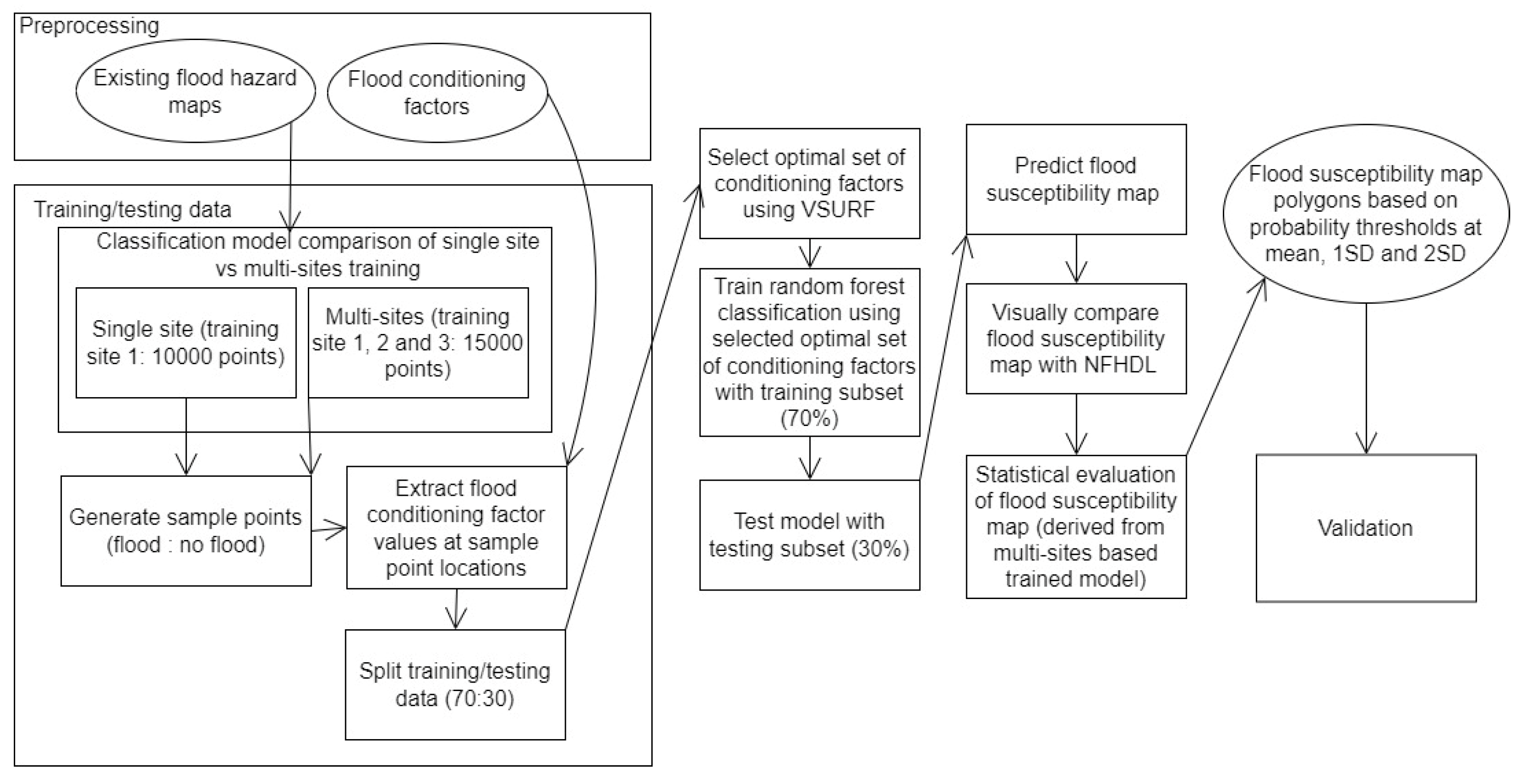
These values were used as thresholds in classifying flooded areas. All the predicted pixels that fall above these thresholds were classified as flooded areas to create the final flood susceptibility map polygons across the capital region. To validate our final flood susceptibility map polygons, we visually compared these with the new NFHDL maps, particularly at the locations of spatial gaps within the FDRP maps. The NFHDL maps provide a much greater coverage within our study area for the validation purpose with the Quebec side starting from the west end up to a few kilometers before the east end of the study area. For the Ontario side, the NFHDL maps start from a few kilometers west of training site 2 up to a few kilometers before the east end of the study area. We demonstrated our complete methodology using the flowchart shown in Figure 4.

3. Results

3.1. VSURF Output for Single Site and Multi-Sites Training

VSURF selects the same combination of flood conditioning factors for both single site and multi-sites training. Based on VSURF optimization, elevation, HAR, distance to river, and surface geology are the best combination of flood conditioning factors as predictors of flood within the training sites. However, we chose to exclude surface geology as it is the weakest of the selected flood conditioning factors and has a relatively low resolution (25 m) resulting in artifacts in the predicted flood susceptibility map.

3.2. Single Site Training vs. Multi-Sites Training Performances against NFHDL Maps

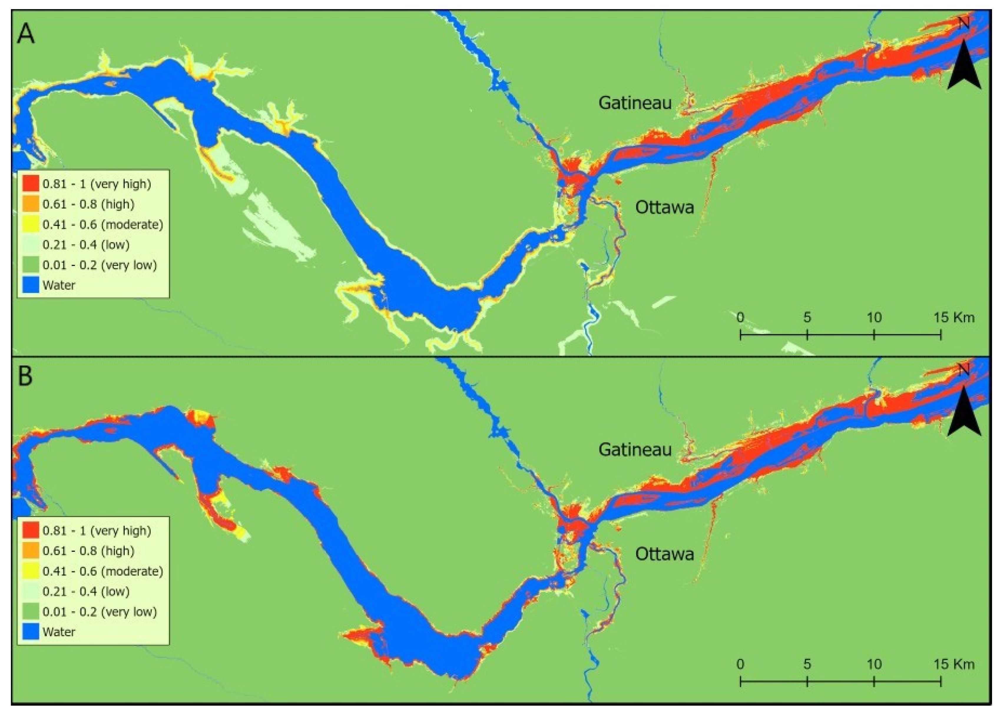
Overall, the random forest classification produces high accuracy flood prediction based on both single site training (accuracy 0.972, kappa coefficient 0.944, Table S1) and multi-sites training (accuracy 0.971, kappa coefficient 0.943, Table S1). In addition, when visually compared with the new NFHDL maps, both single site training and multi-sites training flood predictions perform very well. Particularly, around the downtown Ottawa–Gatineau region and towards the east of downtown, our flood prediction shows very high accuracy (i.e., very high probability of flood occurrence in red, Figure 5). However, as we go west from the downtown area, the flood prediction accuracy is reduced for the single site training model; for example, at some existing flood locations (on NFHDL maps) the single site training flood prediction shows a lower probability of flood occurrence (flood areas represented with yellow and orange, Figure 5A). However, the multi-sites training flood prediction improves the flood prediction accuracy by increasing the flood occurrence probability to ‘very high’ toward the west of downtown (flood areas represented with red, Figure 5B).

3.3. Statistical Evaluation of Flood Probability Thresholds: Used for Delineating Final Flood Susceptibility Map Polygons

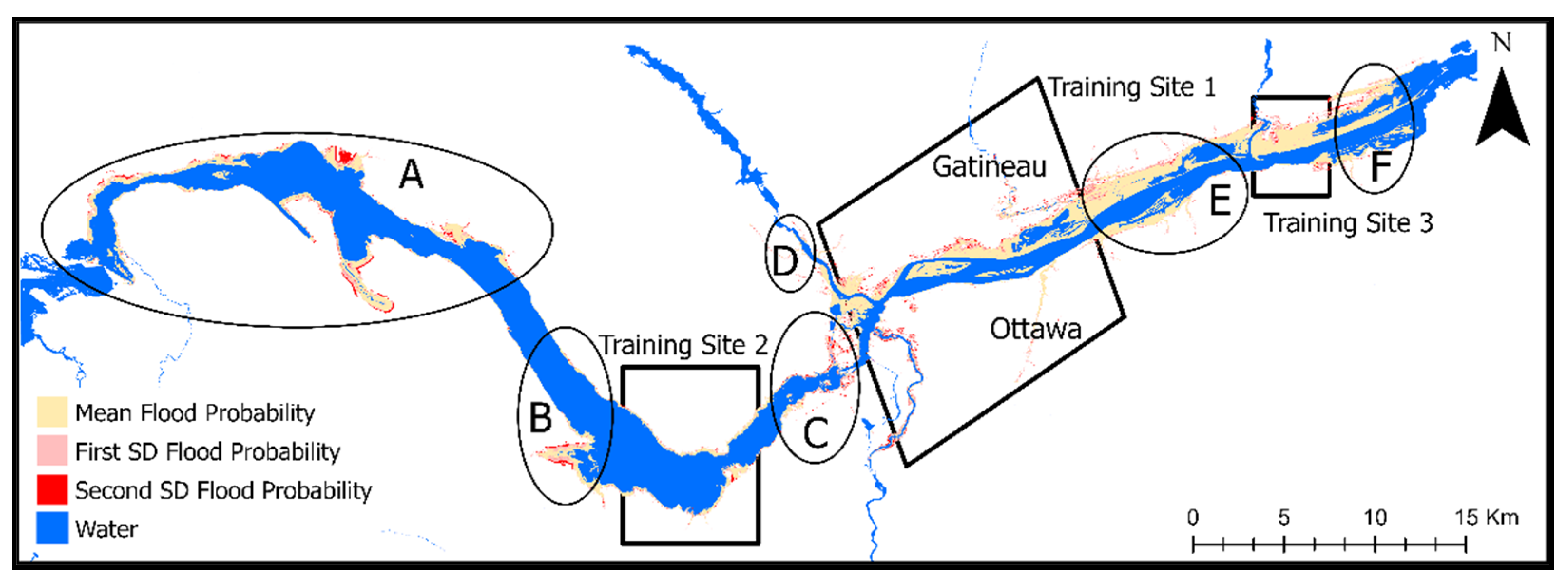
The histogram shows the distribution of flood occurrence probability ranging from 0 to 1 within the existing flood hazard areas (FDRP and RVCA maps, used for training). Values closer to 0 have a low flood occurrence probability and those closer to 1 have a high flood occurrence probability (Figure 6). The histogram shows a mean of 0.935 (very high flood probability) representing ~85% of pixels classified as flood, a one standard deviation of 0.75 (high flood probability) representing 92% of pixels classified as flood, and a two standard deviations of 0.57 (moderate flood probability) representing ~95% of pixels classified as flood (Table S2). All the pixels from the flood susceptibility raster (Figure 5B) falling above these thresholds (i.e., within two standard deviations) were, respectively, classified as flooded areas in a series of flood susceptibility polygons across the capital region (Figure 7).

3.4. Validation of the Final Flood Susceptibility Map Polygons at the Locations of Existing Spatial Gaps within the FDRP Flood Hazard Areas against the NFHDL Maps

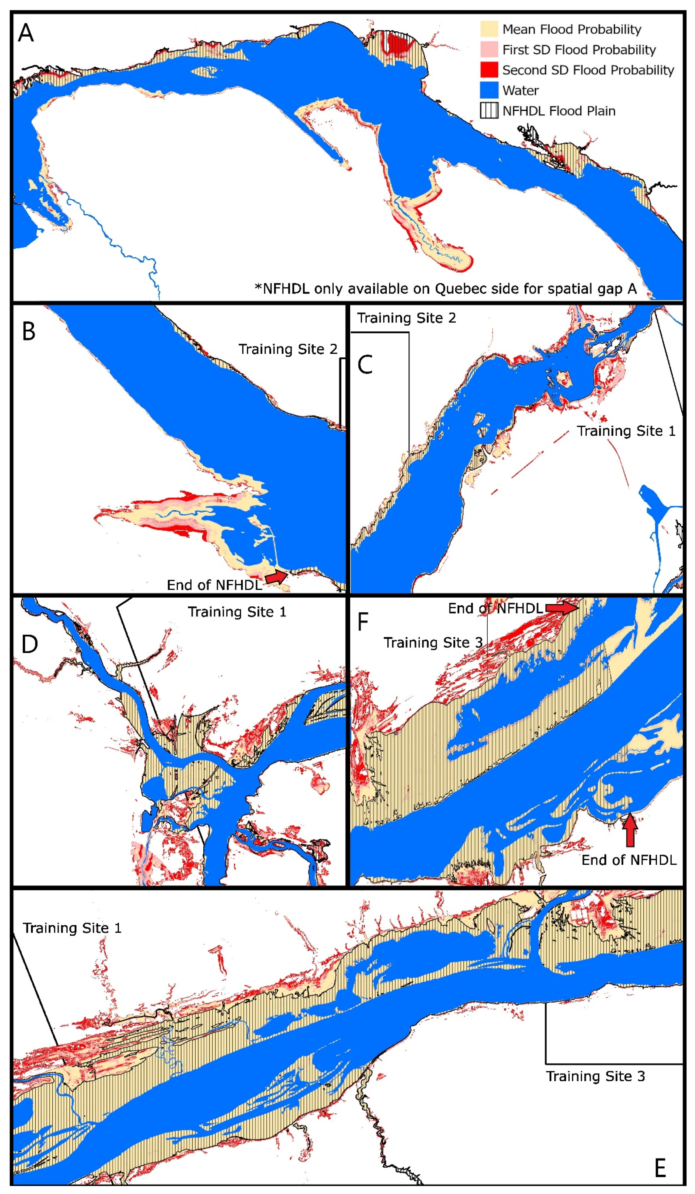
The final flood susceptibility map polygons generated using the flood occurrence probability thresholds of mean, first standard deviation and second standard deviation are shown in Figure 7. Figure 7 also indicates the locations of existing spatial gaps (circles) within the FDRP flood hazard areas, which were used for validating our flood prediction accuracy shown in Figure 8. In the final flood susceptibility map polygons, the mean + first standard deviation flood occurrence probability line up very closely overall with the new NFHDL maps (Figure 8). However, with the second standard deviation, we observe some mismatch (Figure 8). In most locations, the flood predictions (at mean + first standard deviation) match perfectly with the NFHDL maps across the study area. However, some areas, mainly around downtown and toward the far west, show some discrepancies between our flood predictions and the NFHDL maps (Figure 8). In addition, as indicated in Section 2.8 and marked in Figure 8 (spatial gaps A, B, F), some predicted areas are not part of the validation as the NFHDL maps do not have coverages for those areas to validate against.

4. Discussion

4.1. Evaluate Random Forest Classification (Single Site Training vs. Multi-Sites Training) Performance against NFHDL Maps

We find at 1 m resolution, both the single site training (accuracy 0.972, kappa coefficient 0.944, Table S1) and multi-sites training (accuracy 0.971, kappa coefficient 0.943, Table S1) of the random forest classification produces very high accuracy flood susceptibility maps using the same combination of flood conditioning factors (elevation, HAR and distance to river). When compared against the NFHDL maps, both the single site and the multi-sites trained models perform very well with flood prediction in the downtown Ottawa–Gatineau region and east of downtown (Figure 5A,B).
However, west of downtown, flood prediction accuracy decreases for the single site trained model (yellow and orange, Figure 5A), whereas the multi-sites trained model largely improves the overall flood prediction in those regions at existing flood locations (red, Figure 5B). When we analyze the 1 m resolution elevation raster, we see a trend of increasing elevation when moving westward from training site 1 (Figure S3). This trend suggests that there is not sufficient elevation variation in the training and testing dataset used in the single site trained model. We overcame this issue by extending our training and testing data from the two additional sites (training site 2 and training site 3, Figure 3) and the optimized multi-sites trained model demonstrated this when validated against the NFHDL maps west of downtown. The multi-sites trained model improved the prediction accuracy by increasing the flood occurrence probability from moderate (yellow and orange Figure 5A) to very high in those regions (red, Figure 5B). This improvement can be explained by the increased variation of the training and testing data used for the multi-sites trained model. This also indicates that the efficiency of random forest classification in predicting flood is dependent on the training and testing data. Applying a random forest classification should be performed with caution, particularly considering the characteristic of the areas that are predicted compared to the areas that are used for training.

4.2. Final Flood Susceptibility Map Polygons Based on Flood Probability Thresholds and Validating Existing Spatial Gaps within the FDRP Maps against NFHDL Maps

We delineated our final flood susceptibility map polygons using the flood probability thresholds (mean, 1 SD and 2 SD, Figure 7) derived from the multi-sites trained model. When validated, overall, the mean + first standard deviation flood probability thresholds line up very closely with the NFHDL maps whereas the second standard deviation shows some over prediction (Figure 8). However, for the second standard deviation, the probability of flood occurrence is only moderate (2 SD = 0.57). With these results, it can be inferred that the predicted flood susceptibility map (from the multi-sites trained model) is highly accurate as the majority (75.8%) of the flooded pixels were predicted with ~100% flood occurrence probability within the existing flood hazard areas (FDRP and RVCA maps). In addition, 92% of the flooded pixels (at mean + 1 SD threshold) were within the high to very high flood occurrence probability range (Table S2). In order to determine the overall performance of random forest classification to fill in the spatial gaps between existing flood hazard maps, we validated our multi-sites trained model outside of the training sites 1, 2 and 3. We show the spatial gaps within the FDPR maps with circles on Figure 7 and compare our flood predictions at those locations against the NFHDL maps (Figure 8).
Overall, our final flood susceptibility map polygons (at mean + 1 SD threshold) line up accurately against NFHDL maps at the locations of those spatial gaps within the FDRP flood hazard areas. However, we see some mixed results in some areas around central Ottawa–Gatineau in spatial gaps C (eastern portion) and D, and some areas far west of Ottawa–Gatineau in spatial gap A (Figure 8). The discrepancies in the central Ottawa–Gatineau areas (spatial gaps C and D) can be explained by the fact that this is the most urbanized region within our study area and additional high resolution flood conditioning factors, such as land cover or imperviousness, might have improved the accuracy. For spatial gap A in the far west in Pontiac, Quebec, this area is 30 km away from the nearest training site 2, therefore, it is expected that flood conditioning factors in these areas may vary compared to our training sites. This may have resulted in some discrepancies in flood prediction in spatial gap A. Some overall discrepancies can be further explained as the training data from the Quebec side is based on much older FDRP maps compared to the more recent RVCA map on the Ontario side. The lack of consistency between these maps (e.g., different modeling tools and parameters and data used in FDRP were much older) are likely to have contributed to some of the discrepancies seen in Figure 8.
On the other hand, we notice our flood predictions match very closely with the NFHDL maps when we go outside the central Ottawa–Gatineau areas both westward in spatial gaps B and C and eastward in spatial gaps E and F (Figure 8). This may be explained partially by the lack of urbanization near the river, making our flood conditioning factors sufficient for this classification exercise without needing additional predictors. Our overall high accuracy flood prediction results imply that high resolution elevation-based data (e.g., elevation and HAR) and distance to river are powerful base flood conditioning factors.

5. Conclusions

Our analysis demonstrates that random forest classification is able to predict high accuracy flood susceptibility maps at high resolution (1 m). When validated against the recently produced NFHDL flood hazard maps (Figure 8) provided by Natural Resources Canada, we demonstrated that our multi-sites training random forest classification yields a highly accurate flood susceptibility map and can fill in spatial gaps between existing flood hazard maps. We argue that random forest classification is a time and cost-effective solution to harmonize and extend existing flood hazard maps. Our flood susceptibility map of the Ottawa–Gatineau region will provide a guide and contribute toward Natural Resources Canada’s long-term goal of developing spatially continuous flood susceptibility mapping at the watershed scale. This map is already applicable and beneficial for flood mitigation efforts and urban planning in the capital region. We have made our flood susceptibility maps’ polygons publicly available at https://doi.org/10.6084/m9.figshare.21424944. Since flood hazard maps are expensive to generate, this study will benefit similar situations around the globe. Although this random forest classification framework was applied within a Canadian study area it can be replicated elsewhere with relevant data.

Supplementary Materials

The following supporting information can be downloaded at: https://www.mdpi.com/article/10.3390/w14233801/s1, Figure S1: The flood conditioning factors (part 1); Figure S2: The flood conditioning factors (part 2); Figure S3: 1 m resolution elevation raster across the study area; Table S1: Random forest classification performance for single site vs. multi-sites trained models; Table S2: The distribution of the predicted flood probability and the cumulative pixels (derived from the multi-sites training random forest classification model) within the existing flood hazard areas (FDRP and RVCA maps, used for training).

Author Contributions

S.A.B.: Conceptualization, Methodology, Software, Validation, Formal Analysis, Investigation, Resources, Data Curation, Writing—Original Draft, Writing—Review and Editing, Visualization, Project Administration, Funding Acquisition. C.P.B.: Conceptualization, Writing—Review and Editing, Supervision. H.M.: Conceptualization, Resources, Writing—Review and Editing, Supervision, Project Administration, Funding Acquisition. All authors have read and agreed to the published version of the manuscript.

Funding

This research was funded by the Department of Natural Resources Canada, contribution number: 20220028.

Data Availability Statement

We have made our flood susceptibility maps’ polygons publicly available, which can be accessed here: https://doi.org/10.6084/m9.figshare.21424944. All data sources to verify the conclusions of this work have been included. The flood conditioning factors data are both open-access and available online or can be requested. The 1 m resolution elevation data for the province of Quebec can be found at https://mffp.gouv.qc.ca/les-forets/inventaire-ecoforestier/foret-ouverte-wms/ (accessed on 1 March 2021). The 1 m resolution elevation data for the Ontario side can be requested from the City of Ottawa. The 30 m resolution elevation data can be found at https://maps.canada.ca/czs/index-en.html (accessed on 1 March 2021). Distance to river can be derived from the national hydro network data found at https://www.nrcan.gc.ca/science-and-data/science-and-research/earth-sciences/geography/topographic-information/geobase-surface-water-program-geeau/national-hydrographic-network/2136 (accessed on 1 March 2021). Distance to road can be derived from the road network data for Ontario (https://open.ottawa.ca/datasets/road-centrelines/explore) (accessed on 4 April 2021) and Quebec (https://www.gatineau.ca/portail/default.aspx?p=publications_cartes_statistiques_donnees_ouvertes/donnees_ouvertes/jeux_donnees/details&id=872107914) (accessed on 4 April 2021). Land cover data can be found at https://open.canada.ca/data/en/dataset/4e615eae-b90c-420b-adee-2ca35896caf6 (accessed on 1 March 2021). Surface geology data can be found at https://doi.org/10.4095/295462 (accessed on 4 April 2021). The FDRP and NFHDL flood hazard maps can be requested from Dr. Heather McGrath ([email protected]) at Natural Resources Canada. The RVCA flood hazard map can be requested from Brian Stratton ([email protected]) at Rideau Valley Conservation Authority.

Acknowledgments

We acknowledge the Department of Natural Resources Canada for funding this research, contribution number: 20220028. We acknowledge all the datasets used for flood analysis which are both publicly available and acquired through agreement (Rideau Valley Conservation Authority).

Conflicts of Interest

The authors declare no conflict of interest.

References

  1. Schiermeier, Q. Increased Flood Risk Linked to Global Warming. Nature 2011, 470, 316. [Google Scholar] [CrossRef] [PubMed] [Green Version]
  2. Ciszewski, D.; Grygar, T.M. A Review of Flood-Related Storage and Remobilization of Heavy Metal Pollutants in River Systems. Water. Air. Soil Pollut. 2016, 227, 239. [Google Scholar] [CrossRef] [PubMed] [Green Version]
  3. Mcgrath, H.; Stefanakis, E.; Nastev, M. Sensitivity Analysis of Flood Damage Estimates: A Case Study in Fredericton, New Brunswick. Int. J. Disaster Risk Reduct. 2015, 14, 379–387. [Google Scholar] [CrossRef]
  4. Bush, E.; Lemmen, D.S. (Eds.) Canada’s Changing Climate Report; Government of Canada: Ottawa, ON, Canada, 2019; ISBN 9780660302225. [Google Scholar]
  5. Gaur, A.; Gaur, A.; Simonovic, S.P. Future Changes in Flood Hazards across Canada under a Changing Climate. Water 2018, 10, 1441. [Google Scholar] [CrossRef] [Green Version]
  6. Ottawa RIVERKEEPER 6 Things You Should Know about the 2019 Flooding—Ottawa Riverkeeper|Garde-Rivière Des Outaouais. Available online: https://ottawariverkeeper.ca/6-things-you-should-know-about-the-2019-flooding/ (accessed on 22 July 2022).
  7. Hodgson, C. Explainer: Is Climate Change the Cause of the 2019 Ottawa River Flooding?—Ecology Ottawa. Available online: https://www.ecologyottawa.ca/2019-05-02-explainer-is-climate-change-the-cause-of-the-2019-ottawa-river-flooding (accessed on 22 July 2022).
  8. Ottawa Riverkeeper Dams. Available online: https://www.ottawariverkeeper.ca/home/explore-the-river/dams/ (accessed on 8 November 2020).
  9. Ottawa River Regulation Planning Board. 2019 Spring Flood—Questions and Answers; Ottawa River Regulation Planning Board: Gatineau, QC, Canada, 2019; pp. 1–18. Available online: https://ottawariver.ca/information/publications/ (accessed on 22 November 2020).
  10. McNeil, D. Ontario Government Report on 2019 Flooding of the Ottawa River. Available online: https://www.merrileefullerton.ca/ontario_government_report_on_2019_flooding_of_the_ottawa_river (accessed on 7 December 2020).
  11. Tehrany, M.; Jones, S.; Shabani, F. Identifying the Essential Flood Conditioning Factors for Flood Prone Area Mapping Using Machine Learning Techniques. Catena 2019, 175, 174–192. [Google Scholar] [CrossRef]
  12. Natural Resources Canada and Public Safety Canada Federal Hydrologic and Hydraulic Procedures for Floodplain Delineation Version 1.0; Government of Canada: Ottawa, ON, Canada, 2019.
  13. Natural Resources Canada and Public Safety Canada Federal Flood Mapping Framework Version 2.0; Government of Canada: Ottawa, ON, Canada, 2018.
  14. Marin Watershed Program Hydrology and Hydraulic (H&H) Modeling. Available online: https://www.marinwatersheds.org/resources/projects/hydrology-and-hydraulic-hh-modeling (accessed on 15 August 2022).
  15. Exponent Hydrology & Hydraulics. Available online: https://www.exponent.com/services/practices/engineering/civil-engineering/capabilities/water-resources/hydrology--hydraulics/?serviceId=13098ca1-18b8-4603-af33-8b88d9905164&loadAllByPageSize=true&knowledgePageSize=7&knowledgePageNum=0&newseventPageSize=7&newseventPageNum=0&professionalsPageNum=1 (accessed on 15 August 2022).
  16. Esfandiari, M.; Abdi, G.; Jabari, S.; McGrath, H.; Coleman, D. Flood Hazard Risk Mapping Using a Pseudo Supervised Random Forest. Remote Sens. 2020, 12, 3206. [Google Scholar] [CrossRef]
  17. Tehrany, M.S.; Pradhan, B.; Jebur, M.N. Flood Susceptibility Mapping Using a Novel Ensemble Weights-of-Evidence and Support Vector Machine Models in GIS. J. Hydrol. 2014, 512, 332–343. [Google Scholar] [CrossRef]
  18. Breiman, L. Random Forests. Mach. Learn. 2001, 45, 5–32. [Google Scholar] [CrossRef] [Green Version]
  19. Ho, T.K. Random Decision Forests. In Proceedings of the 3rd International Conference on Document Analysis and Recognition, Montreal, QC, Canada, 14–16 August 1995; Volume 1, pp. 278–282. [Google Scholar] [CrossRef]
  20. Zhao, G.; Pang, B.; Xu, Z.; Yue, J.; Tu, T. Mapping Flood Susceptibility in Mountainous Areas on a National Scale in China. Sci. Total Environ. 2018, 615, 1133–1142. [Google Scholar] [CrossRef]
  21. Esfandiari, M.; Jabari, S.; McGrath, H.; Coleman, D. Flood Mapping Using Random Forest and Identifying the Essential Conditioning Factors; A Case Study in Fredericton, New Brunswick, Canada. ISPRS Ann. Photogramm. Remote Sens. Spat. Inf. Sci. 2020, 5, 609–615. [Google Scholar] [CrossRef]
  22. Wang, Z.; Lai, C.; Chen, X.; Yang, B.; Zhao, S.; Bai, X. Flood Hazard Risk Assessment Model Based on Random Forest. J. Hydrol. 2015, 527, 1130–1141. [Google Scholar] [CrossRef]
  23. William, B.; Scriven, G. Flood Susceptibility Mapping in the Red River Valley, Manitoba, Using Machine Learning; Natural Resources Canada: Ottawa, ON, Canada, 2019. [Google Scholar]
  24. Shafapour Tehrany, M.; Shabani, F.; Neamah Jebur, M.; Hong, H.; Chen, W.; Xie, X. GIS-Based Spatial Prediction of Flood Prone Areas Using Standalone Frequency Ratio, Logistic Regression, Weight of Evidence and Their Ensemble Techniques. Geomat. Nat. Hazards Risk 2017, 8, 1538–1561. [Google Scholar] [CrossRef] [Green Version]
  25. Kia, M.B.; Pirasteh, S.; Pradhan, B.; Mahmud, A.R.; Sulaiman, W.N.A.; Moradi, A. An Artificial Neural Network Model for Flood Simulation Using GIS: Johor River Basin, Malaysia. Environ. Earth Sci. 2012, 67, 251–264. [Google Scholar] [CrossRef]
  26. Water Science School Impervious Surfaces and Flooding. Available online: https://www.usgs.gov/special-topics/water-science-school/science/impervious-surfaces-and-flooding (accessed on 22 July 2022).
  27. Environment and Climate Change Canada. An Examination of Governance, Existing Data, Potential Indicators and Values in the Ottawa River Watershed; Environment and Climate Change Canada: Gatineau QC, Canada, 2019; ISBN 9780660310534.
  28. Ottawa Riverkeeper Watershed Facts. Available online: https://ottawariverkeeper.ca/watershed-fact/ (accessed on 22 October 2022).
  29. Giovannettone, J.; Copenhaver, T.; Burns, M.; Choquette, S. A Statistical Approach to Mapping Flood Susceptibility in the Lower Connecticut River Valley Region. Water Resour. Res. 2018, 54, 7603–7618. [Google Scholar] [CrossRef]
  30. McGrath, H.; Gohl, P.N. Accessing the Impact of Meteorological Variables on Machine Learning Flood Susceptibility Mapping. Remote Sens. 2022, 14, 1656. [Google Scholar] [CrossRef]
  31. Fernández-Delgado, M.; Cernadas, E.; Barro, S.; Amorim, D. Do We Need Hundreds of Classifiers to Solve Real World Classification Problems? J. Mach. Learn. Res. 2014, 15, 3133–3181. [Google Scholar]
  32. Liaw, A.; Wiener, M. Classification and Regression by RandomForest. R News 2002, 2, 18–22. [Google Scholar]
  33. Natural Resources Canada Flood Mapping Community. Available online: https://www.nrcan.gc.ca/science-and-data/science-and-research/natural-hazards/flood-mapping-community/24229 (accessed on 21 August 2022).
  34. Ahmed, F.; Mikalson, D.; Ghioureliotis, P.; Liu, E.; Larsen, A. Ottawa River Flood Risk Mapping from Shirley’s Bay to Cumberland; Rideau Valley Conservation Authority: Ottawa, ON, Canada, 2014. [Google Scholar]
  35. RVCA Rideau Valley Conservation Authority. Available online: https://www.rvca.ca/ (accessed on 3 April 2022).
  36. Bates, P.D.; Marks, K.J.; Horritt, M.S. Optimal Use of High-Resolution Topographic Data in Flood Inundation Models. Hydrol. Process. 2003, 17, 537–557. [Google Scholar] [CrossRef]
  37. Van Etten, J.; Sumner, M.; Cheng, J.; Baston, D.; Bevan, A.; Bivand, R.; Busetto, L.; Canty, M.; Fasoli, B.; Forrest, D.; et al. Package “Raster”. Spat. Data Sci. 2022. Available online: https://rspatial.org/raster/ (accessed on 13 October 2020).
  38. Wu, Q. Andrew Brown Whitebox. Available online: https://giswqs.github.io/whiteboxR/ (accessed on 3 April 2022).
  39. Čučković, Z. Terrain Position Index for QGIS. Available online: https://landscapearchaeology.org/2019/tpi/ (accessed on 23 October 2022).
  40. Florinsky, I.V. An Illustrated Introduction to General Geomorphometry. Prog. Phys. Geogr. 2017, 41, 723–752. [Google Scholar] [CrossRef]
  41. Mattivi, P.; Franci, F.; Lambertini, A.; Bitelli, G. TWI Computation: A Comparison of Different Open Source GISs. Open Geospat. Data Softw. Stand. 2019, 4, 6. [Google Scholar] [CrossRef] [Green Version]
  42. Metcalfe, P.; Buytaert, W. Upslope.Area: Upslope Contributing Area and Wetness Index Calculation in Dynatopmodel: Implementation of the Dynamic TOPMODEL Hydrological Model. Available online: https://rdrr.io/cran/dynatopmodel/man/upslope.area.html (accessed on 3 August 2022).
  43. Dilt, T. Height Above Nearest Drainage Goes Mainstream in QGIS and ArcGIS. Available online: http://gislandscapeecology.blogspot.com/2020/04/height-above-nearest-drainage-goes.html (accessed on 25 October 2022).
  44. Dilts, E.; Yang, J.; Weisberg, P.J. Mapping Riparian Vegetation with Lidar Data. ESRI ArcUser Winter, 2010; 18–21. [Google Scholar]
  45. O’Connor, J.E.; Grant, G.E.; Costa, J.E. The Geology and Geography of Floods. Am. Geophys. Union 2002, 5, 359–385. [Google Scholar] [CrossRef]
  46. City of Ottawa Index Ottawa (1K) 2015. Available online: https://gsguo.maps.arcgis.com/apps/PublicInformation/index.html?appid=bff582719c85404f9f77a1ef965759cf (accessed on 22 March 2022).
  47. WMS Ministry of Forests, Wildlife and Parks. Available online: https://mffp.gouv.qc.ca/les-forets/inventaire-ecoforestier/foret-ouverte-wms/ (accessed on 22 March 2022).
  48. Open Government Portal Canadian Digital Elevation Model, 1945–2011. Available online: https://open.canada.ca/data/en/dataset/7f245e4d-76c2-4caa-951a-45d1d2051333 (accessed on 3 August 2022).
  49. GeoBase Surface Water Program (GeEAU) National Hydrographic Network. Available online: https://www.nrcan.gc.ca/science-and-data/science-and-research/earth-sciences/geography/topographic-information/geobase-surface-water-program-geeau/national-hydrographic-network/21361 (accessed on 22 March 2022).
  50. City of Gatineau Road Network. Available online: https://www.gatineau.ca/portail/default.aspx?p=publications_cartes_statistiques_donnees_ouvertes/donnees_ouvertes/jeux_donnees/details&id=872107914 (accessed on 3 April 2022).
  51. City of Ottawa Road Centrelines. Available online: https://open.ottawa.ca/datasets/road-centrelines/explore (accessed on 3 April 2022).
  52. Natural Resources Canada 2015 Land Cover of Canada. Available online: https://open.canada.ca/data/en/dataset/4e615eae-b90c-420b-adee-2ca35896caf6 (accessed on 3 April 2022).
  53. Geological Survey of Canada 2014 Surficial Geology of Canada. Available online: https://doi.org/10.4095/295462 (accessed on 5 October 2020).
  54. Kuhn, M. The Caret Package. Available online: https://topepo.github.io/caret/ (accessed on 3 April 2022).
  55. Genuer, R.; Poggi, J.-M.; Tuleau-Malot, C. VSURF: An R Package for Variable Selection Using Random Forests. R J. 2015, 7, 19–33. [Google Scholar] [CrossRef] [Green Version]
  56. Wright, M.N.; Ziegler, A. Ranger: A Fast Implementation of Random Forests for High Dimensional Data in C++ and R. J. Stat. Softw. 2017, 77, 1–17. [Google Scholar] [CrossRef]
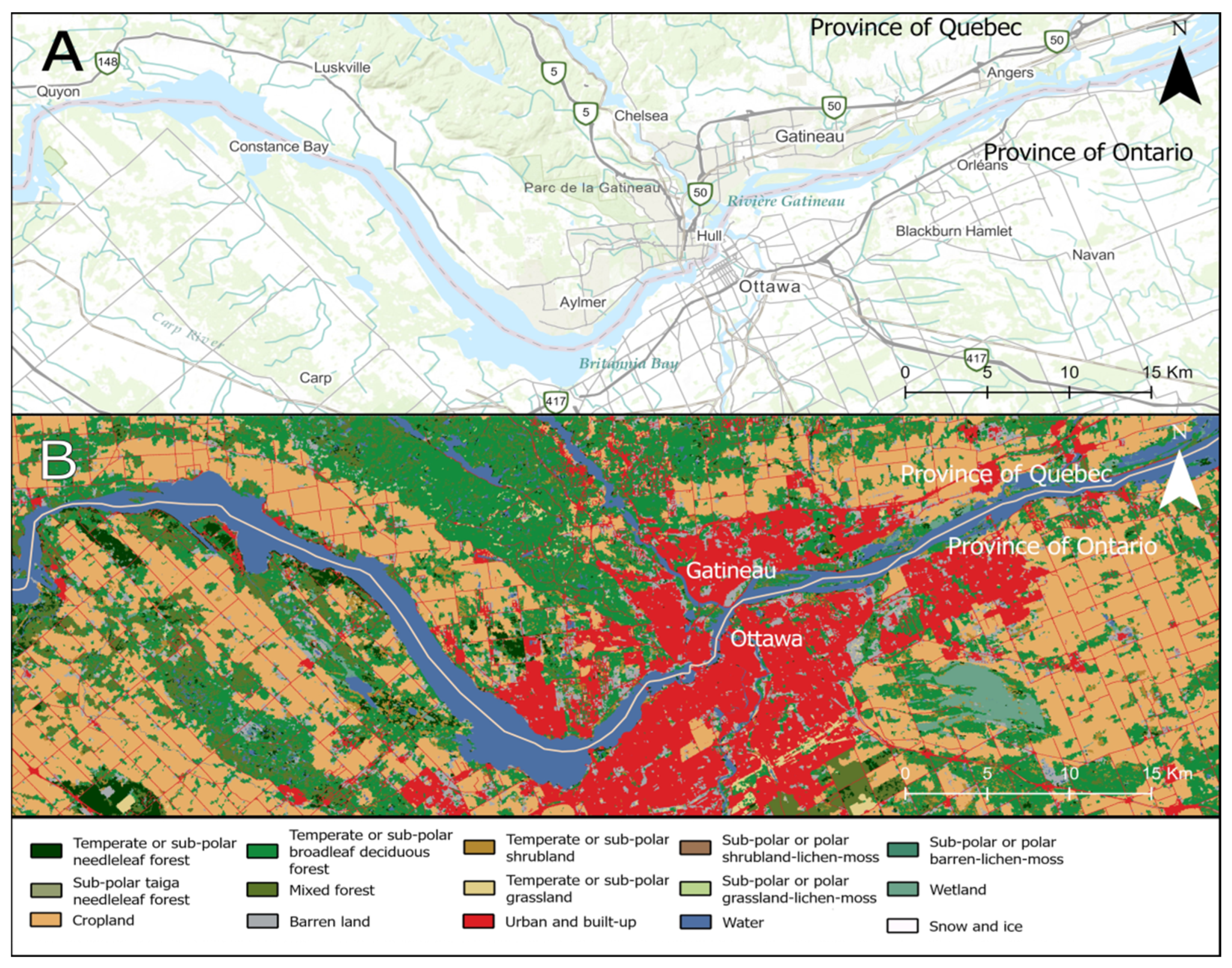
Figure 1. (A) topographic map with main roads and urban areas, from the World Topo Map (Esri, DeLorme, HERE, TomTom, Intermap, increment P Corp., GEBCO, USGS, FAO, NPS, NRCAN, GeoBase, IGN, Kadaster NL, Ordnance Survey, Esri Japan, METI, Esri China (Hong Kong), swisstopo, MapmyIndia, and the GIS User Community). (B) land cover map, from the 2015 Land Cover of Canada (Government of Canada, Natural Resources Canada, Canada Centre for Remote Sensing). The solid line within the Ottawa River represents the provincial boundary between the provinces of Ontario (Ottawa city) and Quebec (Gatineau city), from the Topographic Data of Canada CanVec Series (Government of Canada, Natural Resources Canada, Canada Centre for Remote Sensing).
Water 14 03801 g001
Figure 2. (A) FDRP 100 year flood hazard maps on the Ontario and Quebec side (1980s) with spatial gaps; (B) RVCA 100 year flood hazard map for the Ontario side (continuous); and (C) Training site 1 for random forest classification. Flood hazard maps are compiled from the FDRP (for Quebec side) and RVCA maps (for Ontario side).
Water 14 03801 g002
Figure 3. Multiple training sites: training site 1 (Central), training site 2 (West) and training site 3 (East) using the flood hazards maps (FDRP on the Quebec side and RVCA on the Ontario side).
Water 14 03801 g003
Figure 4. Flowchart describing the training and validation steps of the classification approach.
Water 14 03801 g004
Figure 5. Flood susceptibility maps from the random forest classification model predictions: (A) based on single site training; and (B) based on multi-sites training.
Water 14 03801 g005
Figure 6. Distribution of the predicted flood probability (derived from the multi-sites training random forest classification model) within the existing flood hazard areas (FDRP and RVCA maps, used for training).
Water 14 03801 g006
Figure 7. Final flood susceptibility map polygons generated using the flood occurrence probability thresholds of mean, first standard deviation and second standard deviation The circles (AF) are indicating the locations of existing spatial gaps within the FDRP flood hazard areas, which were used to validate flood prediction accuracy against the NFHDL maps shown in Figure 8.
Water 14 03801 g007
Figure 8. Validation of the final flood susceptibility map polygons at the locations of existing spatial gaps within the FDRP flood hazard areas as shown in Figure 7 with circles (AF). The NFHDL maps do not cover the Ontario side for spatial gap A and most of spatial gap B. For spatial gap F, the NFHDL maps end midway on both the Quebec and Ontario side. The end of the NFHDL coverage is indicated by red arrows.
Water 14 03801 g008
Publisher’s Note: MDPI stays neutral with regard to jurisdictional claims in published maps and institutional affiliations.