Article

A Deep Learning Method Based on Two-Stage CNN Framework for Recognition of Chinese Reservoirs with Sentinel-2 Images

1
Institute of Computing Technology, Chinese Academy of Sciences, Beijing 100086, China
2
International Research Center of Big Data for Sustainable Development Goals, Beijing 100101, China
3
Aerospace Information Research Institute, Chinese Academy of Sciences, Beijing 100101, China
*
Authors to whom correspondence should be addressed.
Water 2022, 14(22), 3755; https://doi.org/10.3390/w14223755
Submission received: 20 September 2022 / Revised: 13 November 2022 / Accepted: 16 November 2022 / Published: 18 November 2022
(This article belongs to the Special Issue Application of Remote Sensing Technology to Water-Related Ecosystems)

Abstract

:
The development of effective and comprehensive methods for mapping and monitoring reservoirs is essential for the utilization of water resources and flood control. Remote sensing has the great advantages of broad spatial coverage and regular revisit to meet the demand of large-scale and long-term tasks of earth observation. Although there already exist some methods for coarse-grained identification of reservoirs at region-level in remote sensing images, it remains a challenge to recognize and localize reservoirs accurately with insufficiency of object details and samples annotated. This study focuses on the fine-grained identification and location of reservoirs with a two-stage CNN framework method, which is comprised of a coarse classification between aquatic and land areas of image patches and a fine detection of reservoirs in aquatic patches with precise geographical coordinates. Moreover, a NIR RCNN detection network is proposed to make use of the multi-spectral characteristics of Sentinel-2 images. To verify the effectiveness of our proposed method, we construct a reservoir and dam dataset of 36 Sentinel-2 images which are sampled in various provinces across China and annotated at the instance level by manual work. The experimental results in the test set show that the two-stage CNN method achieves an average recall of 80.83% nationwide, and the comparison between reservoirs recognized by the proposed model and those provided by the China Institute of Water Resources and Hydropower Research verifies that the model reaches a recall of about 90%. Both the indicator evaluation and visualization of identification results have shown the applicability of the proposed method to reservoir recognition in remote sensing images. Being the first attempt to make a fine-grained identification of reservoirs at the instance level, the two-stage CNN framework, which can automatically identify and localize reservoirs in remote sensing images precisely, shows the prospect to be a useful tool for large-scale and long-term reservoir monitoring.

1. Introduction

Reservoirs, as typical surface water bodies on the earth, are an important part of water-related systems and play a major role in agricultural irrigation, climate regulation and biodiversity studies. Humans have built reservoirs and dams for thousands of years, as the main measures of flood control, water storage, and the generation of hydropower [1].
With the growing demands for clean energy and renewable sources, many countries are developing run-of-river hydropower plants around reservoirs to meet the sustainable development of renewable energy [2]. As for China, the shortages of water and clean energy have prompted the Chinese government to build more dams and reservoirs [3]. According to the first national census for water sources, there have been 97,246 reservoirs built in China as of 2011, with a total storage capacity of more than 8.1 × 10¹¹ m 3 . Meanwhile, the number of big dams in China has reached 23,842 accounting for almost half of the registered big dams worldwide [4], and this number continues to grow today.
As a traditional method to investigate water-related resources, field survey has a limited ability to capture the spatial distribution and temporal variation of water-related resources, especially in some areas with complex landforms [5,6]. When focusing on large areas or long-term tasks, the approach is too time-consuming and costly to implement, thus some existing reservoir distribution across the country or within a province are mainly identified from paper maps or statistical information collected from various sources such as national water resources surveys by Ministry of Water Resources and hydrological monitoring stations [7,8], which make them impossible to adapt to the continuous change of surface water bodies and locations of reservoirs with seasonal and climatic changes as well as the influence of human activities [9,10]. As a result, datasets of geographical coordinates of dams and reservoirs are very limited, even though it has been proved by many studies that reservoirs are essential for the human and natural ecological environment [11].
Different from field survey, remote sensing satellite offers broad spatial coverage and frequent data acquisition on the earth [12], which is a promising technology for monitoring worldwide reservoirs and associated water-related system rapidly, dynamically and cost-efficiently. In addition, remote sensing sensors can obtain multiple spectral imagery in one sample, and the abundant spectral information in visible and infrared bands reflecting the distinguishing characteristics between water and land is invaluable in the recognition of reservoirs and dams in a complex-wide background. Therefore, constructing a comprehensive and effective method based on remote sensing images is a feasible and convenient way to obtain the distribution and geographical coordinates of reservoirs and dams nationwide.
Although remote sensing images can provide abundant information about the earth, it is still a challenge to identify objects of interest accurately in the image with the limited ability of feature representation in image analysis models. Traditional methods for the analysis of the hydrological project information in remote sensing images mainly focus on the design of feature extractors and classifiers by manual work dubbed feature engineering.
Various feature extraction methods have been proposed by researchers in this field. Lu et al. [13] used an algorithm to set a dynamic segmentation threshold to extract surface water bodies in the NIR band data of the MODIS images. The single-band threshold method is one of the most common water extraction methods with a simple principle to implement [14]. However, the results may vary on different data due to changes in seasons, cloudage and water depth, which limit its application in large-scale tasks. For better use of different spectral reflectance characteristics, Gholizadeh et al. [15] evaluated and quantified water quality parameters with data from different sensors on various satellites and other platforms. Costa et al. [16] found that combining SAR and optical images was helpful in water analysis as SAR could provide microwave scattering information of water obviously different from the visible-infrared spectral information. McFeeters et al. [17] proposed the Normalized Difference Water Index (NDWI) to highlight the presence of water in the image and enhance the vegetation and soil features with the prominent reflection in the visible green band and near-infrared radiation.
In terms of classifiers, machine learning algorithms became the dominant methods in remote sensing image analysis at the turn of the century, owing to their ability to project features extracted in images into more distinguishable feature spaces. Several machine learning algorithms, such as Support Vector Machine (SVM), Random Forest (RF), Back-Propagation neural network (BP), Decision Tree (DT), and Gradient Boosting (GB), have been successfully and widely used in aquatic area classification [18,19,20,21,22,23] and have achieved better accuracy [24,25].
In general, the performance of object identification in remote sensing images with traditional feature engineering methods mainly depends on the researcher’s knowledge and experience in the design of feature extractors, which is arduous work and the features extracted are rather limited in generalization. In fact, effective feature extraction has become the bottleneck in traditional image analysis methods. Since AlexNet [26] achieved remarkable accuracy in ImageNet Large Scale Visual Recognition Challenge (ILSVRC) in 2012, deep learning has become an important tool for computer vision tasks such as image classification [27], object detection [28], semantic segmentation [29] and image generation [30], with a notable advantage of learning feature representations in the image. Compared to shallow networks, deep neural networks with multiple hidden layers to capture high-dimensional representation show good generalization and robustness in image identification [31]. Moreover, the rational computing and storage requirement with the network design principle of local connection and weights sharing makes it attractive in image analysis of various fields. At present, deep learning is also widely applied in remote sensing image analysis and presents much better results than traditional feature extraction methods by pure manual work [32,33,34,35,36].
Different from the coarse-grained identification of reservoirs at the region level [1], this study aims to build an automatic and reliable method for fine-grained identification and localization of reservoirs at the instance level, which can precisely extract the geographical coordinates of each reservoir. Therefore, we consider the recognition of reservoirs as an object detection task with deep neural networks in remote sensing images, which not only identifies the reservoir but also localizes each reservoir in the image so that it is convenient to draw the reservoir distribution with the geographical coordinates of reservoirs. Additionally, we design a two-stage CNN framework consisting of classification and object detection for the recognition of Chinese reservoirs in Sentinel-2 images. Moreover, note that being a data-driven model learning method, deep neural networks are usually trained on datasets with a large quantity of annotated samples. Although some remote sensing image datasets containing typical ground targets annotated have been established [37,38,39], there are few annotated image datasets for reservoirs or dams released. So, we also construct a reservoir and dam dataset of Sentinel-2 images across China with annotated reservoirs and dams scattered in more than 20 provinces for model training and verification.
The main contributions of this paper are as follows. (1) A reservoir and dam dataset of national Sentinel-2 images is published, in which thousands of samples scattered in more than 20 provinces are annotated with rectangular bounding boxes by manual work. (2) A two-stage framework based on CNN to classify the aquatic areas and identify the reservoirs and dams at the fine-grained level with precise geographical coordinates in Sentinel-2 images is proposed. (3) The effectiveness of the proposed model is verified by comparison with the visualization and statistics on the constructed dataset and the data from the China Institute of Water Resources and Hydropower Research. 4) A Chinese reservoir distribution in 2020 is generated finally.

2. Materials and Methods
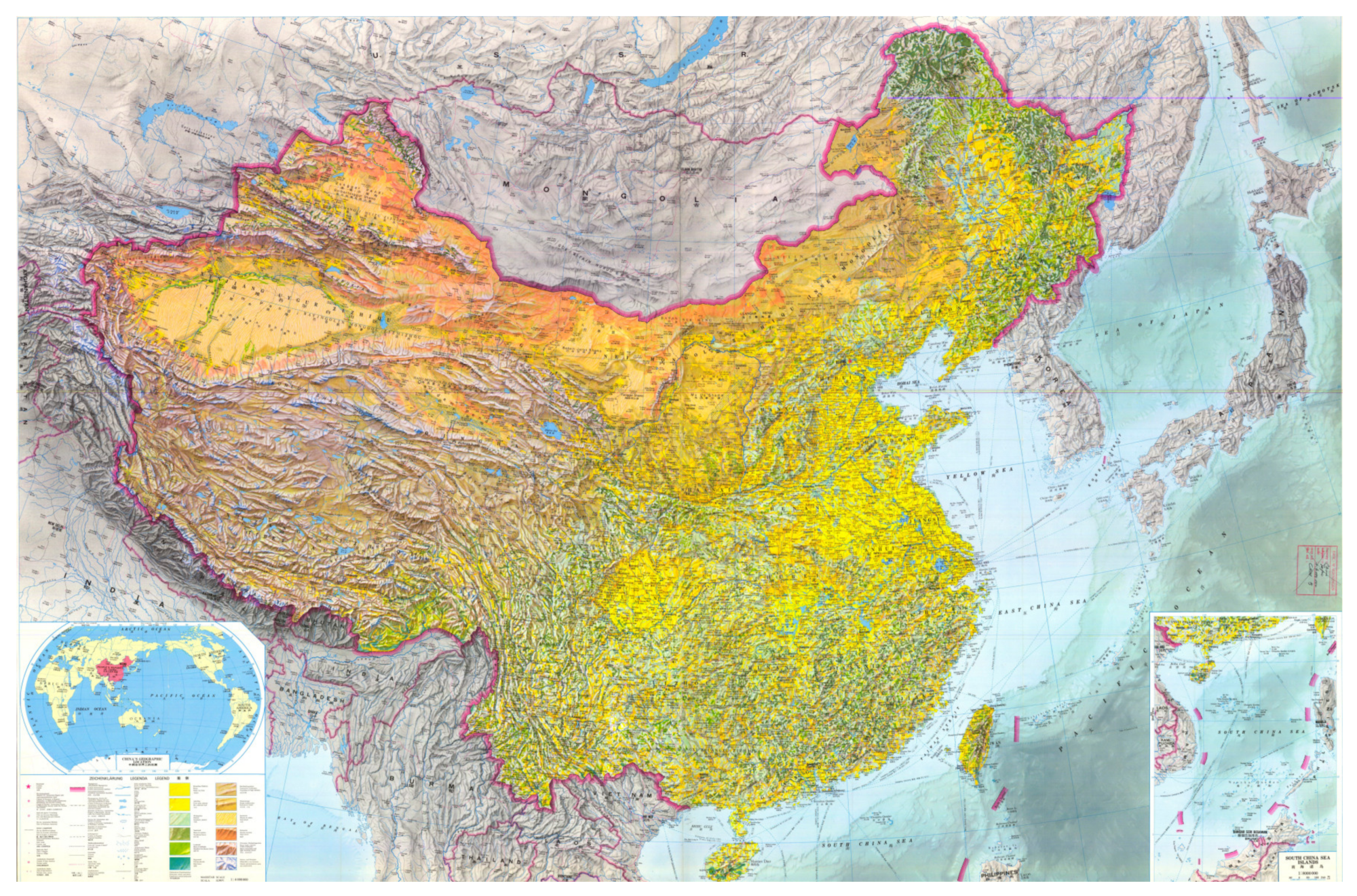
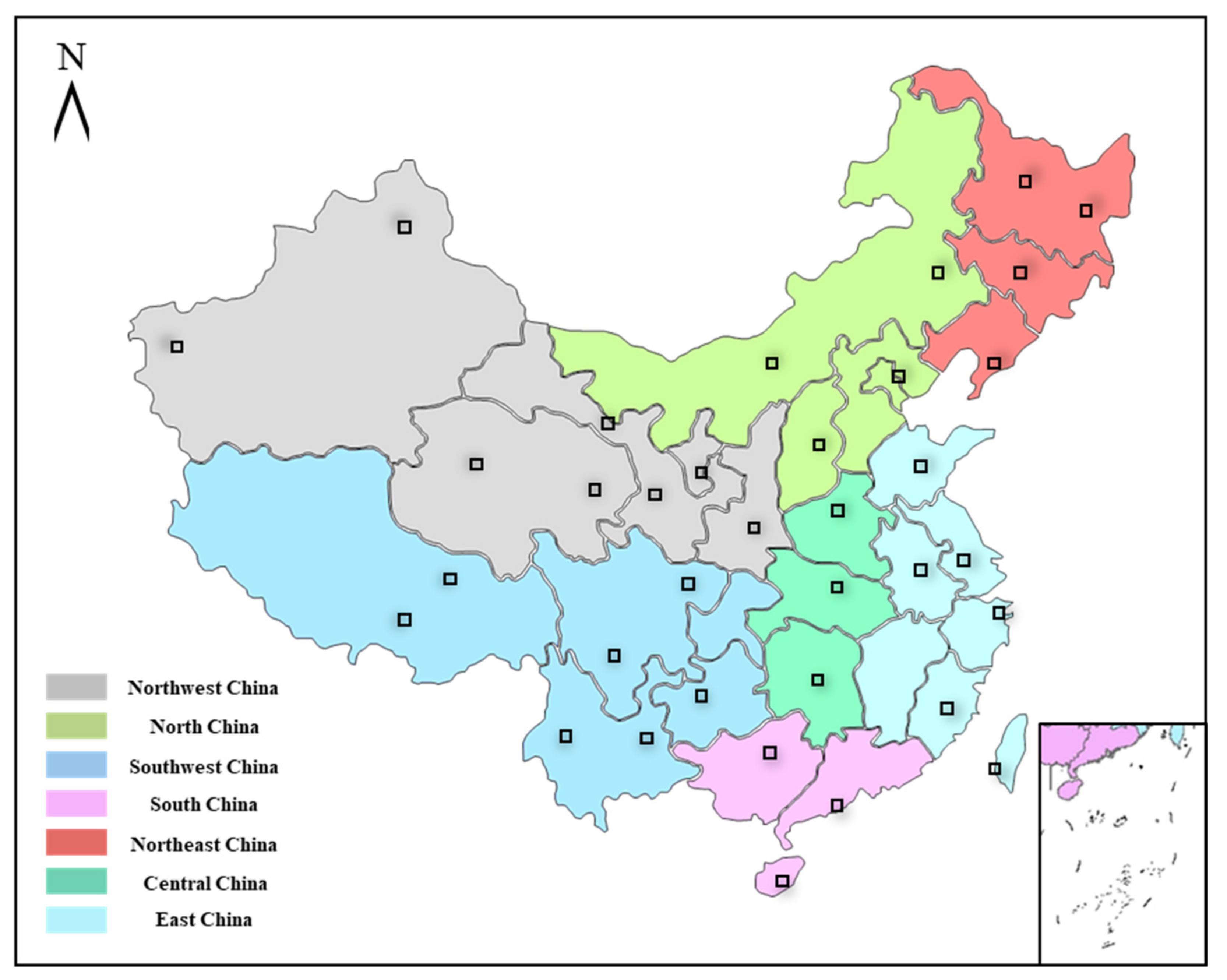
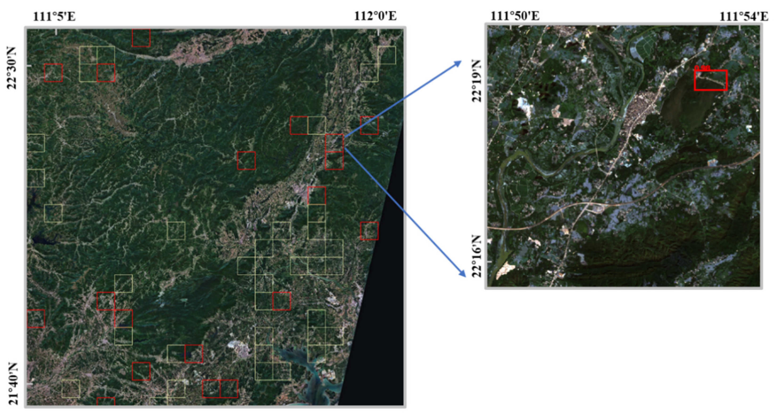
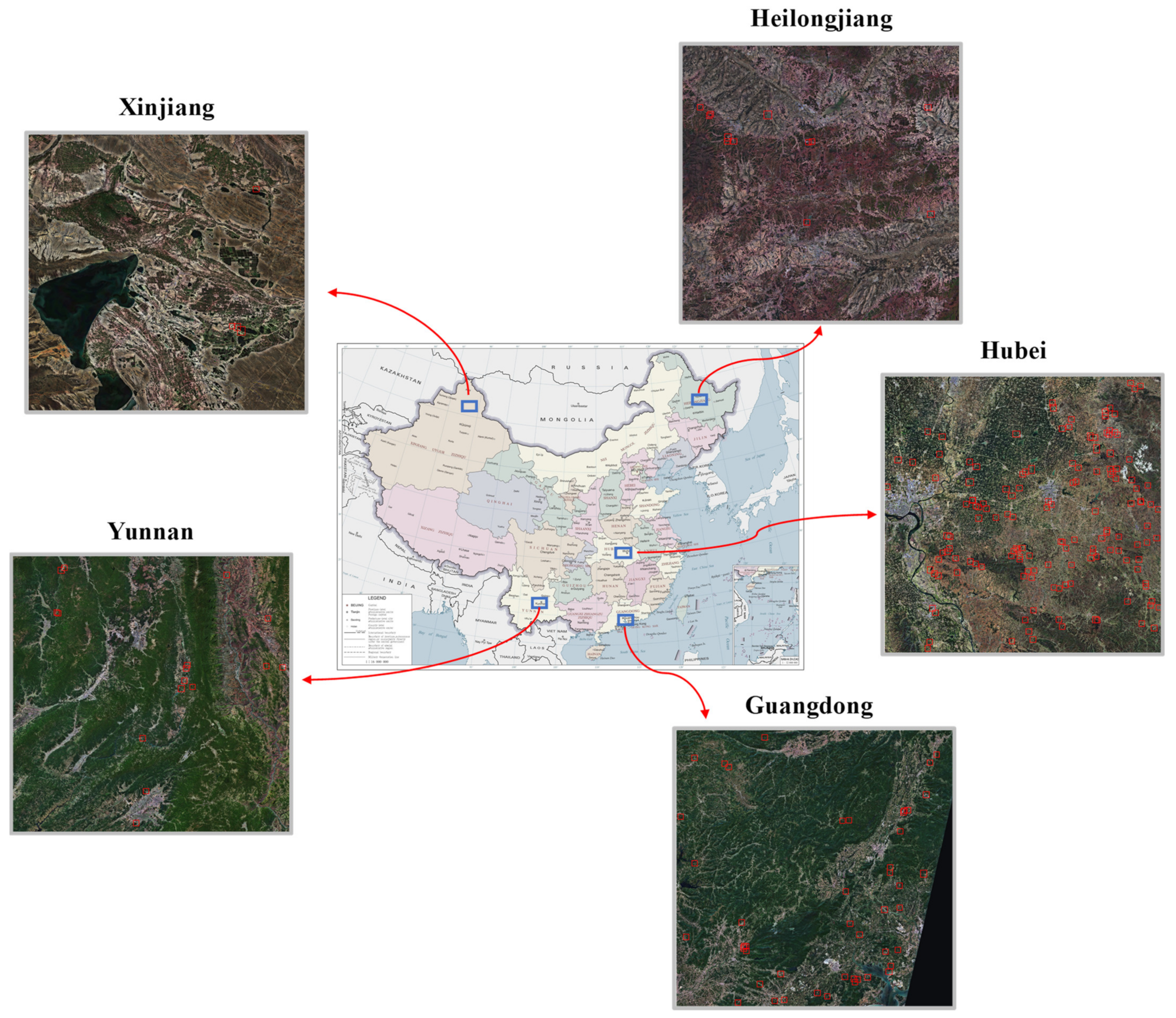
2.1. Study Area

China has a vast territory with a wide range of latitudes and diverse topographic types and mountain ranges are presented in the various terrain.
In this study, we selected China as the study area. As shown in Figure 1, China is located in Eastern Asia (73°330 E–135°20 E, 3°520 N–53°330 N) with complex and diverse landforms including plains, plateaus, mountains, hills and basins, where mountains account for about 2/3 of the country’s area. The terrain of China is high in the west and low in the east, with a roughly three-step distribution. The first step is the Qinghai-Tibet Plateau in the southwest, with an average altitude of more than 4000 m. Between the west of the Great Khingan Mountains, Taihang Mountains, Wu Mountains and Yunnan-Guizhou Plateau and the first step is the second step, which is between 1000–2000 m above sea level mainly consisting of plateaus and basins. To the east of the second step, the land surface above sea level is the third step, which is mainly comprised of hills and plains with altitudes mostly below 500 m. The complex topography in China also leads to the diversity of the combinations between temperature and precipitation, thus forming a variety of climates. Therefore, the distribution of water resources in China is extremely uneven, where water resources in the south are far more concentrated than in the north.

2.2. Datasets

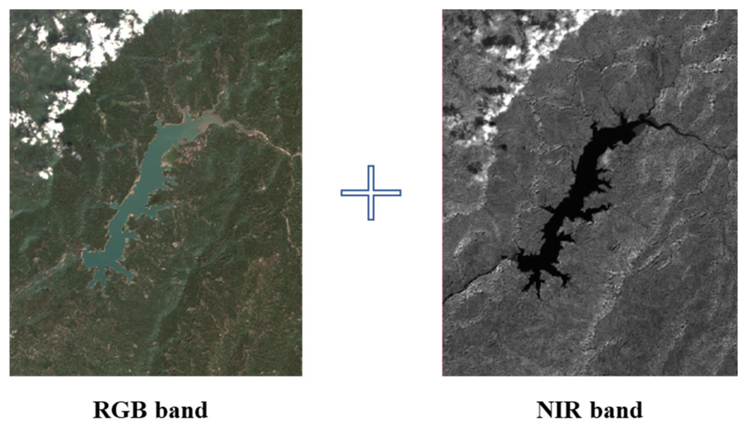
2.2.1. Remote Sensing Satellite Imagery

The data sources for the recognition of reservoirs in China are from Sentinel-2 satellite images captured in 2020 through GEE platform. The Sentinel-2 mission consists of two satellites, Sentinel-2A and Sentinel-2B, with a 180° phase difference, each of which has a total of 13 bands, with a resolution of 10 m, 20 m, or 60 m. A single satellite can complete the revisit within 10 days, so it has a wide range of applications in many fields such as land observation and change detection.
The product of Sentinel-2 satellite mainly includes two levels:
(1)
Level-1C is a Top-of-Atmosphere reflectance product that has gone through orthographic correction and geometric correction but without atmospheric correction.
(2)
Level-2A mainly includes corrected reflectance data of Bottom-of-Atmosphere.
In this study, Sentinel-2 L1C data are downloaded from ESA and then converted to L2A with Sen2Cor [40]. Although Sentinel-2 L2A data can be directly downloaded from ESA, not all of the L2A data that correspond to L1C data are yet available. To create more comprehensive coverage of L2A data, we process locally.
We only make use of RGB band (B4, B3, B2 of Sentinel-2) and near-infrared band (NIR, B8 of Sentinel-2) data of Level-2A product with a resolution of 10m as shown in Figure 2 to construct our dataset for reservoir and dam recognition.
As a result, a total of 1733 Sentinel-2 satellite images of 10,980 × 10,980 pixels covering the whole of China are collected for this study, and each image covers an area of about 100 km × 100 km.

2.2.2. Acquisition of the Training and Testing Dataset

As shown in Figure 3, 36 images of 28 provinces across China excluding special administrative regions and municipalities are sampled from the above 1773 images with 1~2 images in each province to construct the reservoir and dam dataset with labels for the training and verification of our proposed model. These images cover seven geographical areas of China: Northeast China, North China, Central China, East China, South China, Northwest China and Southwest China (Figure 3), and the variety of landforms in China as well. They are divided into a training set of 19 scenes and a test set of 17 scenes randomly with the principle that in each geographical area there are test samples and test images. In this way, a complete and reliable dataset of reservoirs and dams for model training and verification in China is constructed.

2.2.3. Geographical Coordinate Data of Large and Medium-Sized Reservoirs in China
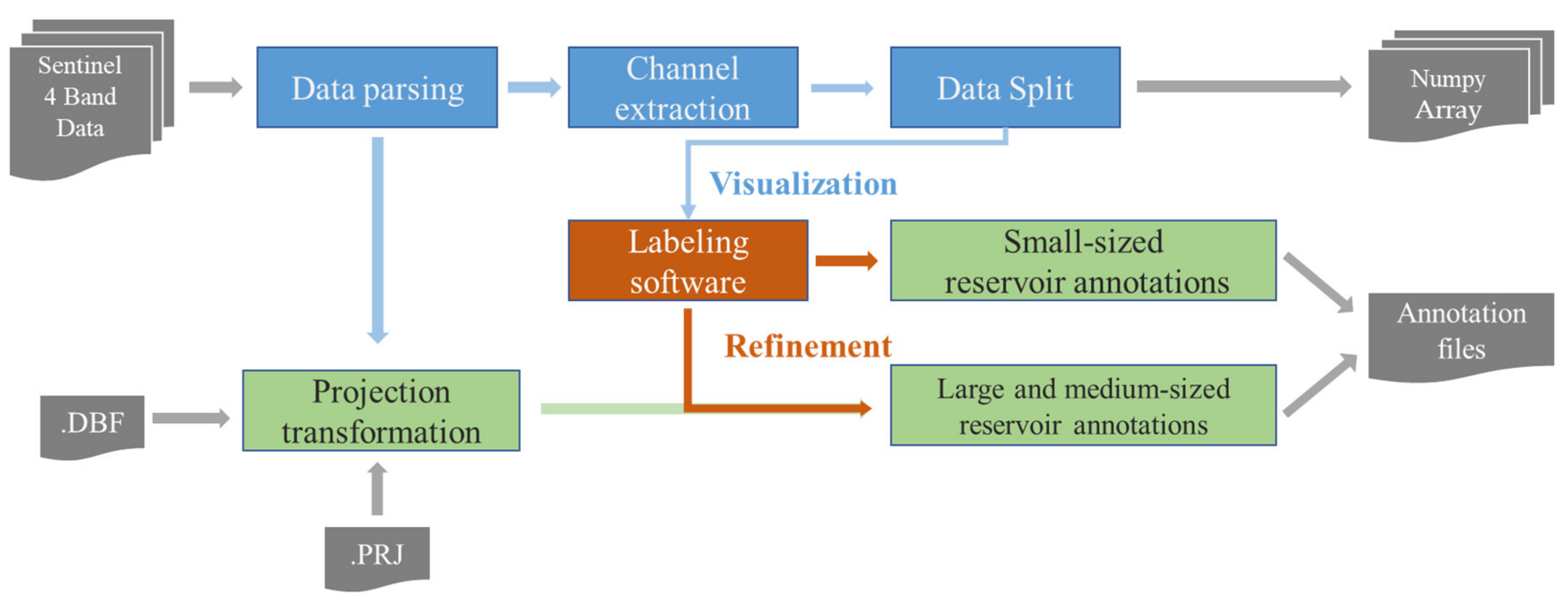
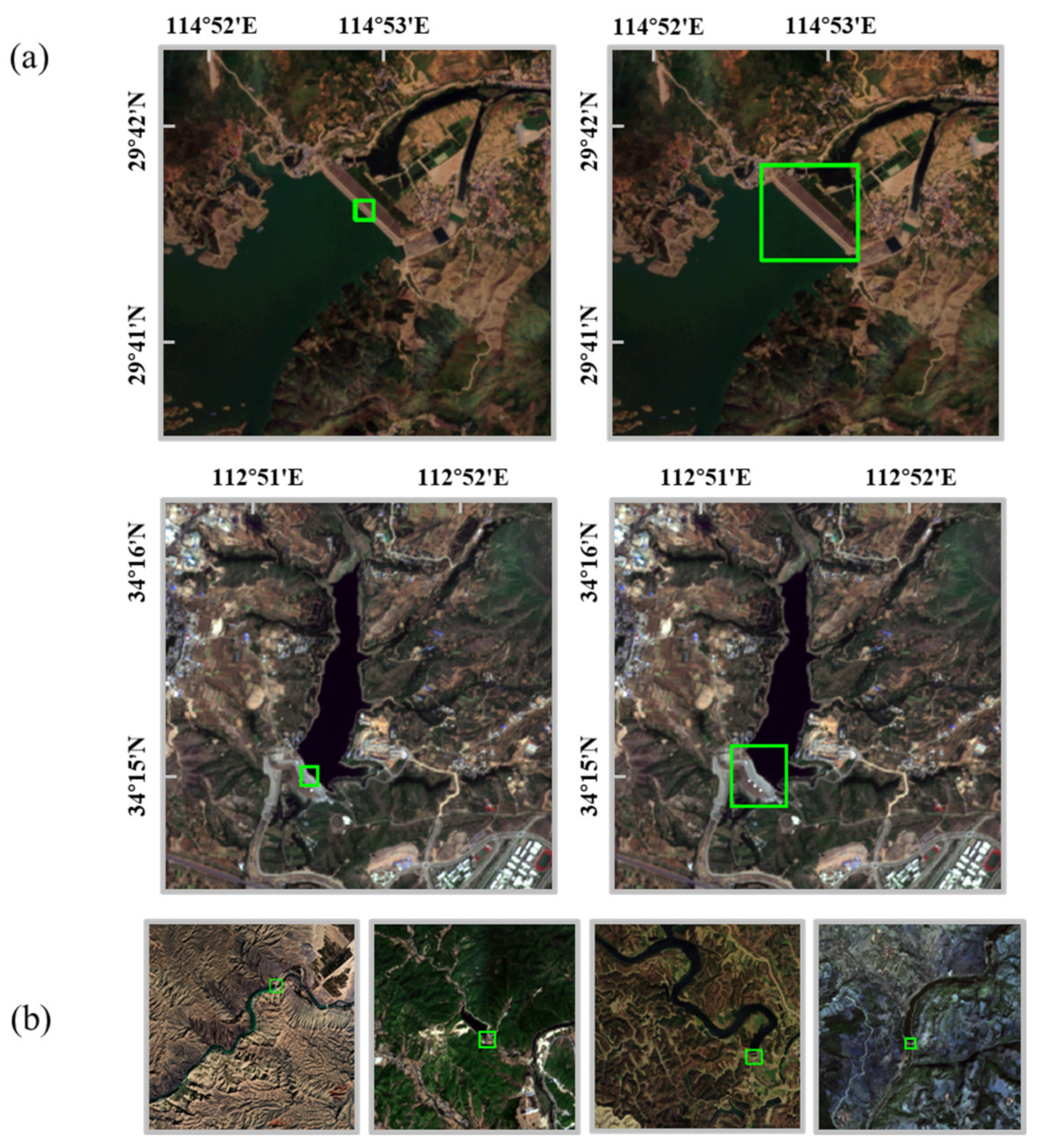
In this study, we employ the statistical information of the geographical coordinates in China released by the China Institute of Water Resources and Hydropower Research in 2019 as auxiliary data for image annotation, and only those large and medium-sized reservoirs with a storage capacity greater than or equal to 100 million cubic meters are included.

2.2.4. Annotations

Data annotation of thousands of reservoir and dam targets is arduous by pure manual work. Since there is no complete dataset of geographical coordinates of reservoirs across China available as described in Section 1, we have to manually annotate reservoirs in the 36 Sentinel-2 images selected in Section 2.2.2. In order to improve the efficiency in data annotation, the geographical coordinate data mentioned in Section 2.2.3 is adopted as a reference for automatic annotation. As the geographical coordinate data is statistically incomplete and its acquisition time is in 2019, different from the time when the Sentinel-2 images were captured, refinement of the automatically generated annotation of the large and medium-sized reservoirs and dams in images has to be performed manually. It is also necessary to supplement the annotation of the small-sized reservoir and dam samples without information on geographical coordinates in images manually for our image-based method of study. More details are shown below.
As shown in Figure 4, the geographical coordinates of large and medium-sized reservoirs and dams in China are projected onto Sentinel-2 images and a rectangular bounding box of a fixed size of 16 × 16 pixels centered on the geographical position is automatically generated for each sample, and these bounding boxes are refined to match the size of each instance by manual work for recognition model training and verification. There may be some discrepancy between the given geographical coordinates of reservoirs and the final refined position. For example, the reservoir has been dried up, or it has been demolished and reconstructed, which also confirms that to draw the distribution of reservoirs and dams only with statistic information is flawed in the long term because it is inconvenient to update. Meanwhile, small reservoirs and dams not included in the dataset released by the China Institute of Water Resources and Hydropower Research are annotated manually. In fact, the number of small reservoirs and dams excluded in the dataset is almost twenty times larger than that of large and medium-sized reservoirs and dams included in the dataset, which also shows that the existing reservoir distribution in China is incomplete and it is necessary to construct a comprehensive and effective method to monitor reservoirs nationwide.
Figure 5a shows the annotation refinement process of the large and medium-sized reservoirs and dams. The left column is the rectangular bounding box with a default size automatically generated according to the geographical coordinates provided by the China Institute of Water Resources and Hydropower Research. Additionally, the right column is the refined bounding box, whose size exactly matches the reservoir and dam for recognition model training and verification and Figure 5b shows some annotations added for small reservoirs and dams by manual work.

2.3. Methods

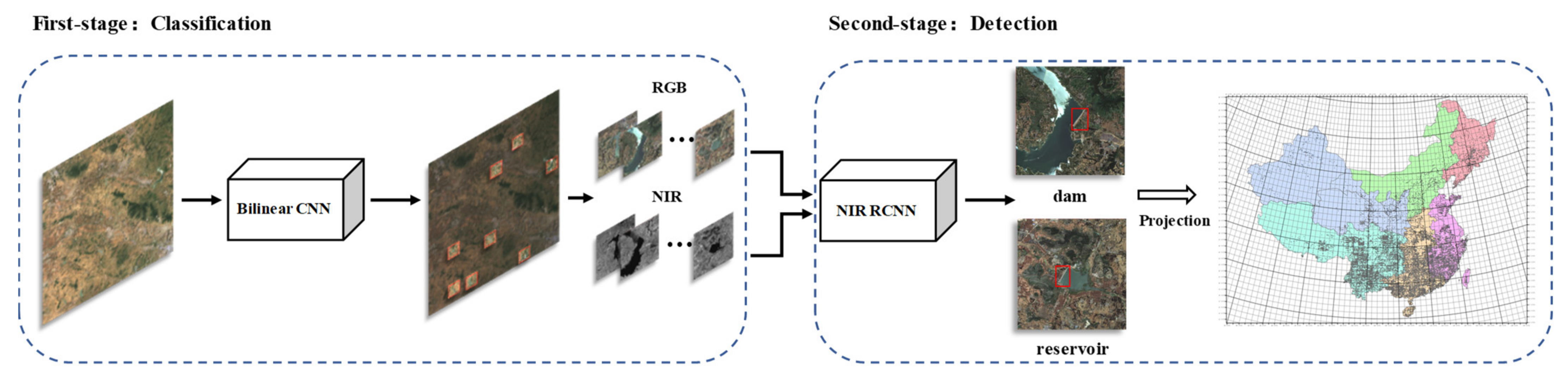
2.3.1. Architecture of the Two-Stage CNN Framework

As mentioned in Section 1, we regard the recognition of reservoirs as an object detection task in computer vision, which aims to localize reservoirs or dam-like constructions in images and output the coordinates of a series of rectangular boxes containing each of them. Different from a natural image, a single remote sensing image captured on a satellite at a distance of hundreds of kilometers from the Earth usually covers a wide ground area in the range of 100   km 2 or even larger, and the proportion of the reservoir or dam in the image is quite small, which makes it difficult to detect directly. Therefore, a two-stage CNN framework is proposed in this study to interpret remote sensing image step by step and extract the information on reservoirs and dams from coarse to fine.
As shown in Figure 6, at the first stage, a coarse-classification network is adopted to filter land areas out of the image, so that the volume of data that has to be processed in the more complicated detection at the second stage is reduced dramatically. Specifically, with the limited memory in GPU, the original image of 10,980 × 10,980 pixels is cut into image patches of 512 × 512 pixels in the order from top to bottom and left to right, which are classified as aquatic areas (water-related region) and land through the coarse-classification network and only patches of aquatic areas that may contain reservoirs and dams are retained. Then, the retained patches are sent to a detection network at the second stage, which corrects errors of samples misclassified at the first stage and localizes reservoirs and dams in patches accurately in the instance level with the form of bounding boxes in pixel coordinates. Finally, a distribution of reservoirs and dams in China is drawn by converting coordinates in pixels to geographical coordinates and projecting them to ArcGIS.

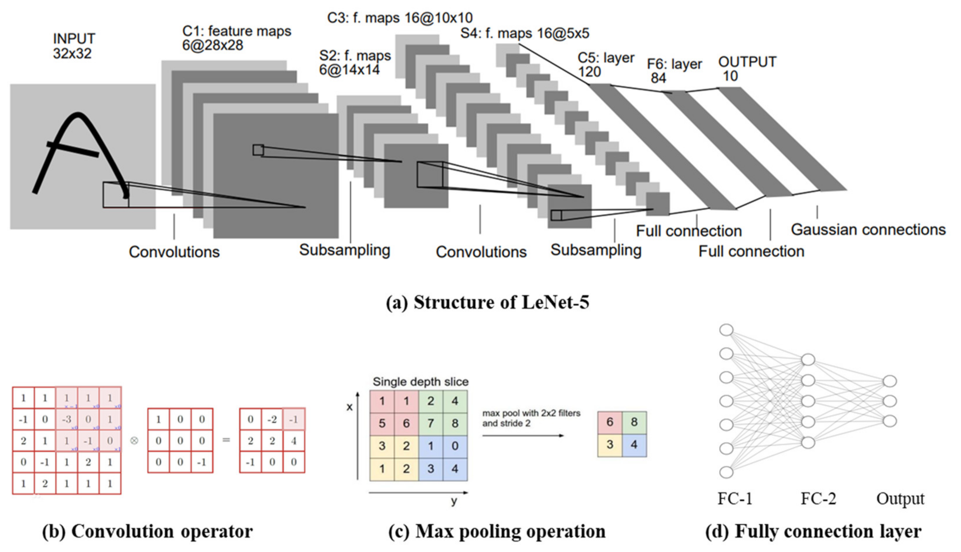
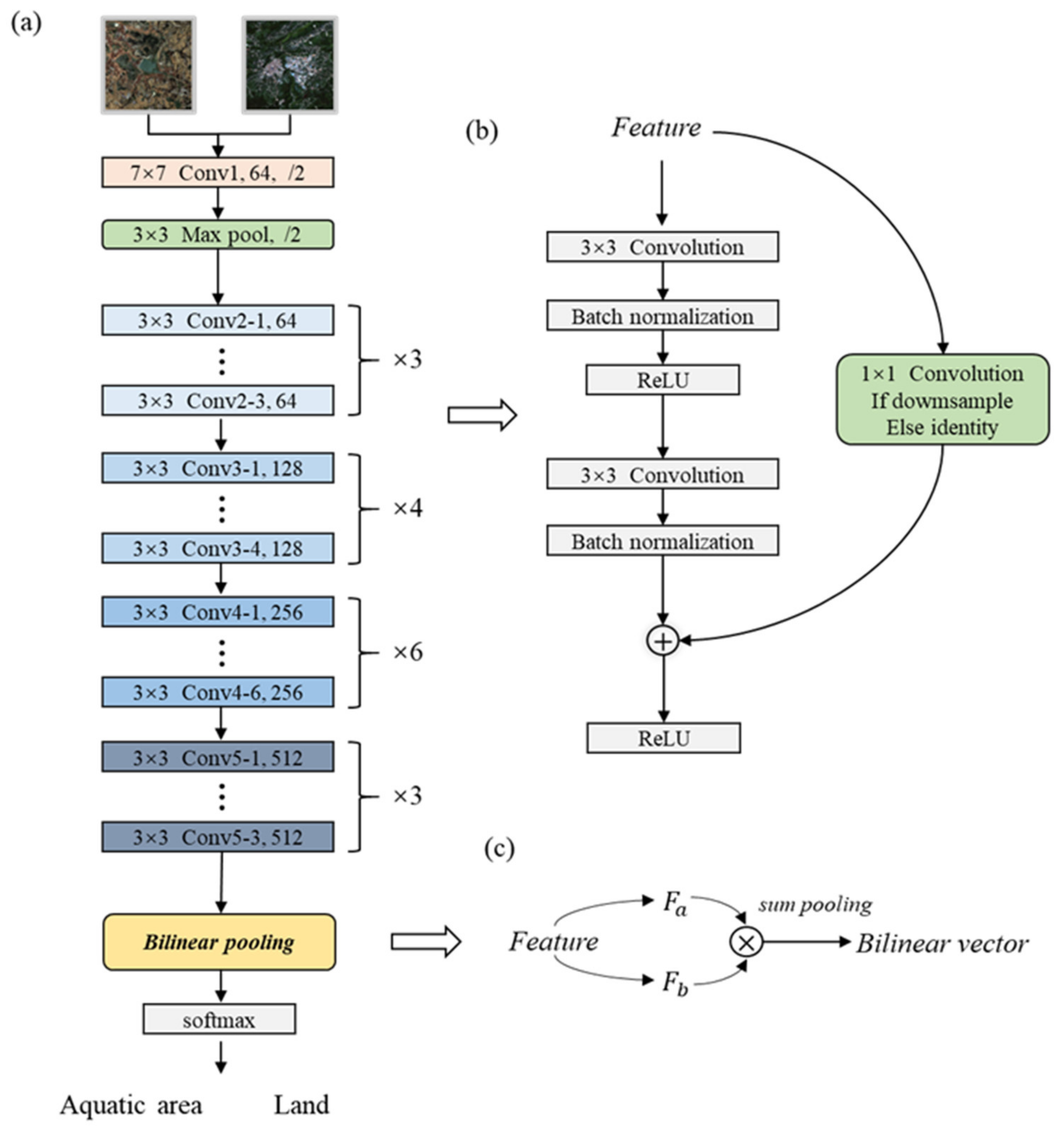
2.3.2. Convolutional Neural Network (CNN)

As mentioned in the introduction, machine learning models based on statistical learning theory, such as Boosting, Logistic Regression, and SVM, usually need characteristics designed by artificial methods to complete identification or prediction tasks because of their restricted ability of feature extraction with only one hidden layer at most, and the advent of deep learning has relieved this problem.
As an important part of deep learning, a deep neural network constructs a multi-layer network to acquire an abstract representation of semantic information in data with multi-level features and achieves better robustness.
The Convolutional Neural Network (CNN) is a deep neural network with a convolutional structure, which is mainly composed of three hierarchical structures: (a) a convolutional layer, a pooling layer and a fully connected layer as depicted in Figure 7a which shows a structure of LeNet-5 for recognition of handwriting [31]; (b) Figure 7b shows the process of convolution; Figure 7c shows the process of max pooling; Figure 7d shows fully connection layer.

2.3.3. Classification of Aquatic Areas and Land

At the first stage of the coarse-classification network, the input is the 512 × 512 image patches(Figure 8), and a bilinear CNN network with a backbone of ResNet34, which has good discrimination between the aquatic area and land images is adopted as shown in Figure 9.
ResNet [27], also known as residual network, is the winner of the 2015 ILSVRC. It solves the problem of gradient disappearance in very deep neural network training with a concept of residual learning and achieves better performance. ResNet has a variety of network structures, and ResNet34 (Figure 9a,b) is selected for the classification task in this study for its light weight.
Bilinear CNN was originally used for fine-grained image classification tasks [41]. Different from traditional CNN, the bilinear CNN network performs a bilinear pooling operation on features extracted by the backbone network for classification. As shown in Figure 9c, first, a bilinear feature fusion is operated for the features in the same position on the feature map. Then, the sum pooling operation is performed on the vectors obtained to form the bilinear vector for classification. This method is considered to be able to integrate spatial information in different locations to obtain a more fine-grained feature representation, which is beneficial for the classification of aquatic and land areas because the Bilinear CNN model can obtain a stronger response in aquatic areas, although it usually occupies a relatively small part in images.

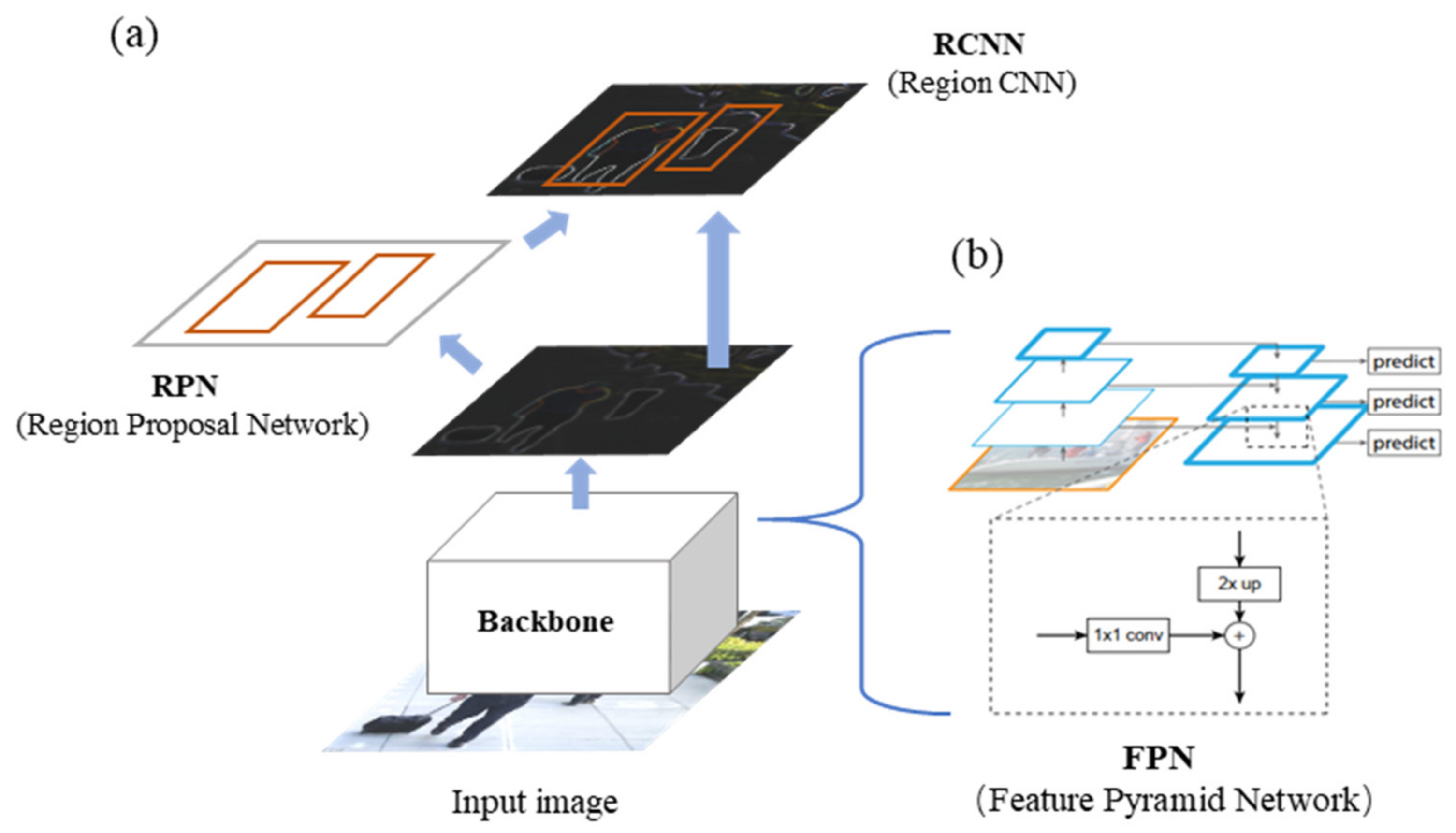
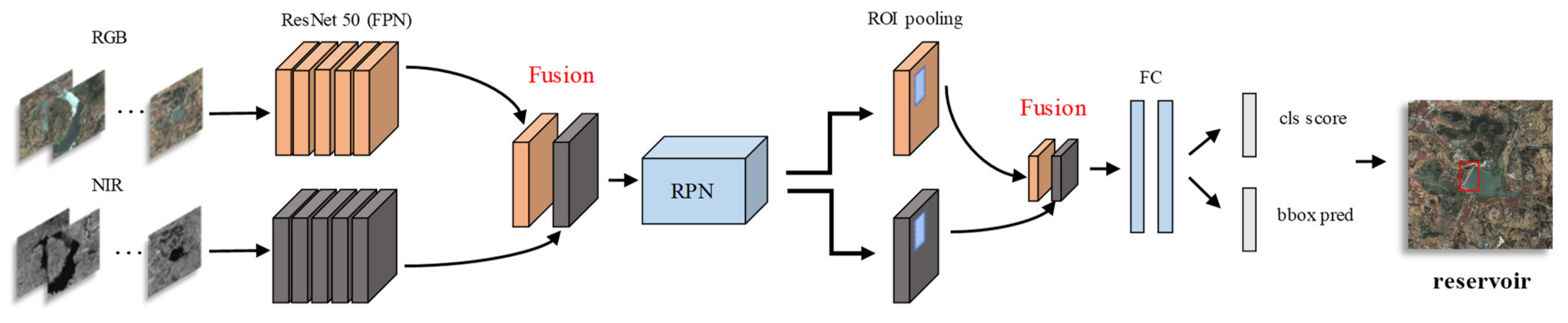
2.3.4. Detection of the Reservoirs and Dams

The detection network of the second stage receives patches classified as aquatic areas at the first stage, i.e., image patches retained in the first stage, which probably contain reservoirs or dams, and makes an accurate identification and localize each instance of the targets.
In this part, the most commonly used two-stage detection network Faster RCNN [28] is adopted in this object detection task, whose major difference from a typical classification network is a regression head to locate objects. Therefore, the detector pays more attention to the local regions and is more fine-grained in feature representation in comparison with image classifiers.
Faster RCNN consists of three parts: backbone of ResNet 50 [27] with FPN [42], RPN network and RCNN network. As shown in Figure 10a, the backbone network aims to extract basic features in images for RPN and RCNN networks. RPN network generates raw proposals with the features extracted by the backbone network and learns to fit the ground truth of the targets (labeled bounding boxes) for the first time. The RCNN network further extracts feature vectors according to the position of raw proposals on the feature map and decodes them into the final category and position vectors of objects.
While ResNet50 has the same architecture as ResNet34 in Section 2.3.3, the difference is that the basic residual block of ResNet34 has changed to a bottleneck module, which deepens the number of network layers and reduces the number of parameters and training time.
In the original Faster RCNN, both the RPN network and RCNN network are based on the single high-level feature map with a high downsampling rate, which is not friendly to small objects, especially in remote sensing images. In order to solve the shortcomings of the object detection algorithm when meeting with multi-scale changes, FPN uses the inherent multi-scale and hierarchical structure of the deep convolutional network to construct the feature pyramid (shown in Figure 10b) to complete the connection between low-level semantics and high-level semantic information from top to bottom, which effectively maintains the detailed information of small targets and improves the performance of detection in minimal additional consumption
As shown in Figure 11, in this study, we design NIR RCNN to make use of the multi-spectral characteristics of Sential-2 images, in which the backbone network and RCNN network extract features of the NIR band data and RGB band data separately, then these features are fused for classification and regression in RPN and RCNN. Further, the fusion operation is completed by feature concatenation between RGB and NIR channels. RPN generates unified proposals based on the fused backbone features, then RCNN extracts the ROI (Region of interest) features separately at the same position on the RGB and NIR feature maps through ROI pooling and performs another fusion with these ROI features. Subsequent experiments show that the usage of NIR band data, along with RGB data, in recognition of reservoirs and dams achieves better performance than the usage of RGB data alone as a result of the reflection characteristics of the water in the NIR band.

2.3.5. Implement Details

Data: As mentioned in the second paragraph of Section 2.3.1, the actual input of the two-stage framework for training and testing is 512 × 512 image patches segmented from 10,980 × 10,980 TIF images, and we obtain 4756 positive samples (patches with reservoirs and dams) and 58,746 negative samples (patches without reservoirs or dams) in the labeled dataset constructed for model training and test. Since aquatic only occupies a small part of the land area in China, the number of positive samples of reservoirs and dams turns out to be far less than that of negative samples. In addition to this, we also introduce 15 TIF images in Hubei Province with reservoirs and dams annotated (with 2222 positive samples) in model training, and finally, there are a total of 4633 positive samples and 31,105 negative samples in the training set while 2345 positive samples and 27,641 negative samples in the test set.
Training of classification network at the first stage: To reduce the influence of extreme imbalance in the numbers of positive and negative samples in the image coarse-classification task at the first stage, the training data is composed of all positive samples and randomly sampled negative samples at a ratio of 1:10 in training set with a total of 46,330 samples, and the test data consists of all 29,986 samples (positive samples and negative samples) in the test set.
Training of the detection network at the second stage: all 4633 positive samples are used as the training data in the detection network, and samples classified as aquatic areas by the classification network at the first stage are used as the test data.
The cross-entropy loss is adopted as the classification loss of networks of the first and second stages of our framework, and the regression loss of the detection network at the second stage is smooth L1. The SDG optimizer is employed at both stages, with the initial learning rate of 0.01, and the weight decay is 1 × 10⁻⁴ and 5 × 10⁻⁴, respectively. CosineAnnealingWarmRestarts is adopted as a learning rate adjustment strategy with restarting cycles of 10 and 30 epochs. The batch size of the classification network is 128 and the detection network is 16, which takes about 3 h to train on a Quadro RTX 6000 GPU with 24 GB of VRAM.

3. Results and Discussion

In this section, we will report the result of our two-stage CNN method for reservoir and dam detection in Section 2 and evaluate its performance in two aspects as follows:
(1)
To evaluate the model on the dataset with image annotations we constructed in Section 2.2.2.
(2)
To compare the detection results with the geographical coordinates of the large and medium-sized reservoirs and dams released by the China Institute of Water Resources and Hydropower Research in Section 2.2.3.
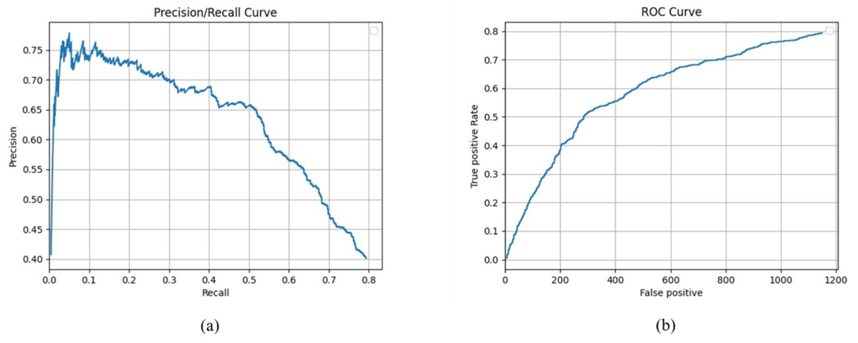
3.1. Metrics

Three common metrics in image classification and detection tasks are used in performance evaluation, i.e., recall, precision and overall accuracy.
For convenience, a confusion matrix is introduced first. The confusion matrix is actually a matrix with elements of the classification/detection results of the model, i.e., the number of samples correctly classified/detected and incorrectly classified/detected by the model.
Take the confusion matrix for binary as an example, where the first category is positive, and the second category is negative (usually background). If the model predicts correctly, it is recorded as True, otherwise, it is False. The elements of a confusion matrix are a combination of these four basic terms (with a specific explanation of the evaluation in the first/second stage network) as shown in Table 1:
  • TP: True Positive (correctly classified aquatic area images/detected reservoir targets)
  • FP: False Positive (misclassified aquatic area images/misidentified reservoir targets)
  • FN: False Negative (incorrectly classified as land images/undetected reservoir targets)
  • TN: True Negative (correctly classified land images)
Table 1. The definition of the Confusion matrix.
AnnotationPositiveNegative
Prediction
PositiveTP (True Positive)FP (False Positive)
NegativeFN (False Negative)TN (True Negative)
Precision and recall are defined as follows:
Precision = TP TP + FP
Recall = TP TP + FN
For the coarse-classification network at the first stage, the precision and recall listed above are related to image patches, i.e., image-level evaluation. When the network predicts an image patch as an aquatic area as well as the ground truth is also, it is recorded as a TP sample, and so on. In addition, the overall accuracy is also adopted in the evaluation of the first-stage model.
Overall   accuracy = TP + TN TP + TN + FP + FN
For the detection network at the second stage, the precision and recall are related to reservoirs or dams, i.e., instance-level evaluation. If a rectangular bounding box predicted by the network intersects with the ground truth bounding box, it is regarded as a TP sample, or, conversely, it is an FP sample. All the bounding boxes output by the detection network are calculated in this way. Since the second category is background, there is no TN indicator. In addition to this, an indicator of the F1 score is introduced as a harmonic value to evaluate the model from different perspectives.
F 1   score = 2 TP 2 TP + FP + FN = 2 × precision × recall precision + recall

3.2. Evaluation on the Constructed Dataset with Labels

3.2.1. Accuracy Assessments of the First-Stage Classification Network

For the coarse-classification network in the first stage, we achieve a recall of 85.16%, a precision of 24.34% and overall accuracy of 78.13% at score threshold = 0.05 with the usage of Bilinear CNN described in Section 2.3.3. It is worth noting that for the coarse-classification network, a lower threshold of classification score is usually set to guarantee a high recall of image patches containing reservoirs or dams to make sure positive samples be preserved as much as possible. Although the precision of the network at the first stage is relatively low, it still removes about 50% of negative samples as shown in Figure 12, the yellow and red boxes represent the output of the classification network that may contain reservoir or dam targets, which accelerates inference of complicated detection of reservoirs and dams at the second stage. Furthermore, different thresholds of classification score to adapt to tasks with different accuracies are also tested as shown in Table 2.

3.2.2. Accuracy Assessments of the Second-Stage Detection Network

For the detection network in the second stage, the retained image patches (left of Figure 12) are received as input of the NIR RCNN described in Section 2.3.4 to make a more complicated detection (right of Figure 12) and to obtain rectangular boxes containing the objects.
Finally, we obtain the detection results of 17 scene images in the test dataset across seven geographic regions in China constructed in Section 2.2, Figure 13 shows the results of some regions.
Table 3 is the metrics of our algorithm at score threshold = 0.2, which achieves great results in the seven national geographic regions with an average recall of about 80% and a precision of about 40%. In particular, the results in the Eastern regions with abundant water resources are better than average, while the results are relatively worse in the Northern and Western regions since it is difficult for the model to learn the potential characteristics of reservoirs and dams there with insufficient training samples. Meanwhile, the model achieves the best results in the central region because there exist various reservoirs and dams in the location of the Yangtze River basin.
We also show the PR curve and the ROC curve to evaluate the performance of our algorithm in multi-view. As shown in Figure 14, (a) is the PR curve where the horizontal axis represents Recall, and the vertical axis represents Precision, which reflects the overall performance of the model under different confidence scores; (b) is the ROC curve, which reflects the relation of the false positive and the true positive rate in object detection and it can be considered as the sensitivity curve of the model to positive examples.
As for the results, in the case of unbalanced data of positive and negative samples used in this study, the PR curve of the model still has a right-convex trend, and the ROC curve has a left-convex trend (means great performance with a better ability to distinguish the positive and negative samples, better performance), which also proves the applicability of our algorithm in recognition of reservoir and dam. Noting that since the first-stage classification network is adopted the end point of the PR curve is not recall = 1, because some patches of ground truth are discarded at this stage.
The visual analysis of the results is given in Figure 15. Different geographic regions in China present different types of landforms, thus the appearance of the image is quite different. Traditional methods with features designed by manual work such as thresholding, manual feature designing, etc., are effective only for imagery of a single area but is difficult to apply for the imagery of different areas in the whole country. In contrast, our algorithm with CNN can accurately identify and localize reservoirs and dams in different geographic regions (or different provinces) with the background of various landforms across China, and the prediction of the model (Red bounding boxes) is basically coincident with the ground truths (Green bounding boxes) in most cases.
Although our algorithm is effective for the recognition of typical reservoirs and dams, limited by the amount of data, there are still some bad cases of missed detections or false alarms with an atypical object. As shown in Figure 16, (a) missed with a unique-shape reservoir; (b) and (c) misidentified with beach and bridge, respectively, which have a similar appearance with the dam-like construction; (d) missed a reservoir under complex landforms; (e) missed a small reservoir. Among these bad cases, (a,d,e) are scarce samples in the dataset so it is difficult for the model to learn to discriminate it, while (b,c) need to acquire contextual information to determine whether it is a reservoir.

3.2.3. Ablation Study

In this section, a performance comparison between the improved algorithm described in Section 2.3 and its corresponding baseline is presented.
For the coarse-classification network in the first stage, the accuracy comparison between Bilinear CNN and CNN with the backbone of ResNet 34 is shown in Table 4. The accuracy of Bilinear CNN is significantly higher than CNN, with Recall 0.77% higher, Precision 3.90% higher and Overall accuracy 5.03% higher. We believe it is thanks to the bilinear pooling operation of Bilinear CNN, which models the relationship between pixels on original feature maps to make the small-scale aquatic area more prominent while land images and images containing large areas of water such as lakes and rivers are excluded.
For the object detection network in the second stage, the information of RGB and NIR channels are integrated in NIR RCNN network with the backbone and ROI feature fusion strategy, and Recall, Precision and F1 score is increased by 2.7%, 2.61% and 2.92%, respectively, compared with Faster RCNN as shown in Table 5. We believe that the performance improvement should be attributed to the introduction of specific features of water in the NIR band brought by the dual-stream network structure, and the fusion operation can explicitly take advantage of these features. Among them, the backbone feature fusion operation plays a major role, because the characteristics of dam-like construction are not discriminative in the NIR channel, and their identification mainly depends on the data of the RGB channel. By the way, When the fusion operation is deprecated, the performance degenerates to be the same as Faster RCNN.

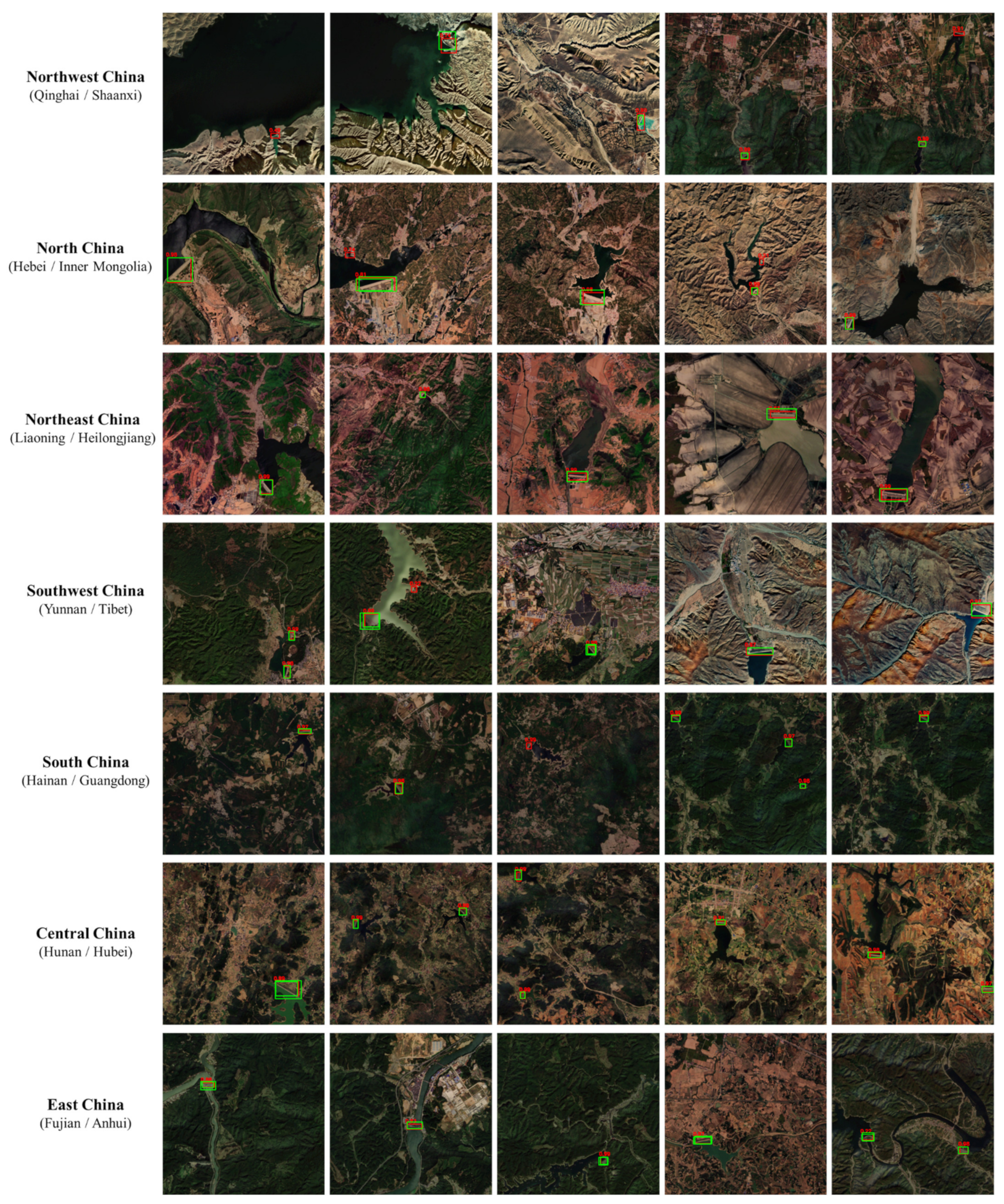
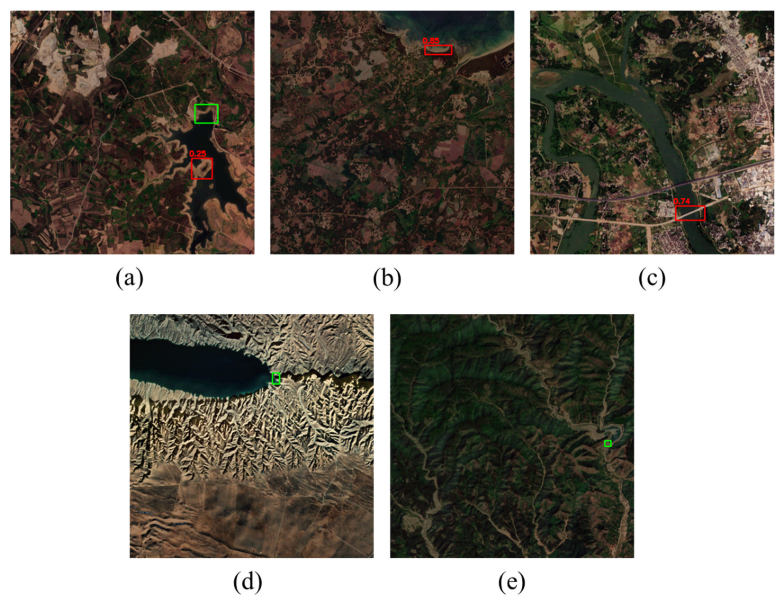
3.3. Comparison with Data Released by the China Institute of Water Resources and Hydropower Research

Inference of reservoir and dam recognition algorithm in 1733 Sentinel-2 images captured in 2020 across China (mentioned in Section 2.2.1) is completed by the two-stage framework models with the best configurations of Bilinear CNN and NIR RCNN in Section 3.2.3 and the distribution of reservoir in China is drawn with the result as shown on the left side of Figure 17 with 34,821 objects, while on the right side shows the distribution of 4662 large and medium-sized reservoirs released by the China Institute of Water Resources and Hydropower Research and the recall of the proposed method reaches about 90% in point-to-point comparison.
It is noteworthy that our proposed method identifies more reservoirs and dams than those released by the China Institute of Water Resources and Hydropower Research and field surveys, partly because small reservoirs are not annotated or included in the latter data. Another reason is that the acquisition time of the latter data does not match with the time when these Sentinel-2 images were captured, and errors may occur in the case of time delay, especially at long intervals. Even so, the geographical distribution of reservoirs obtained with the algorithm in this study is consistent with that provided by the China Institute of Water Resources and Hydropower Research, which also verifies the effectiveness of our algorithm in an aspect.
Our algorithm can automatically obtain the location of the aquatic area of interest and further identifies and localizes reservoirs and dams so long as the captured remote sensing images are fed into the model, which is more suitable for long-term reservoir monitoring over a wide area compared with the method of field survey. It is also a useful tool for the automatic annotation of reservoirs and dams in remote-sensing images.

4. Conclusions

This study aims to realize an efficient method for large-scale and long-term reservoir monitoring. Considering the dynamic nature of remote sensing images covering a wide geographical area, we propose a CNN-based two-stage reservoir recognition algorithm based on remote sensing images of Sentinel-2. First, an image dataset of Sentinel-2 across China that is suitable for model training and verification in deep learning is constructed, in which reservoirs and dams are annotated at the instance level by a combination of manual work and geographical information of reservoirs released by the China Institute of Water Resources and Hydropower Research. Then, according to the imaging characteristic of wide geographical areas in remote sensing, Bilinear CNN is adopted as a coarse classifier to filter land areas out of the input and retain patches of aquatic areas as regions of interest to keep a balance between the accuracy and the speed of inference speed. The detection network of NIR RCNN is designed to identify and localize reservoirs and dams in patches of regions of interest by integration of the multi-spectral information of Sentinel-2 image with the dual-stream network structure and achieves a remarkable improvement in accuracy. Finally, the proposed method is verified in two aspects. One is to test the model on the constructed dataset with images sampled across China, and it achieves an average recall of 80.83% and a precision of 40.56%. We also obtain the metrics at different score thresholds, obtain PR and ROC curves, and give the analysis of visualization results to verify the effectiveness of the method. Another one is to compare the identification result of the model with the geographical coordinates of reservoirs provided by the China Institute of Water Resources and Hydropower Research, and it reaches a recall of about 90% in point-to-point comparison. The above experiments confirm that the proposed method has advantages in generalization and robustness as well as speed in automatic processing compared with traditional methods. The distribution of reservoirs in China is drawn with the identification result of this method, which shows the prospect of this method being a substitute for the arduous and costly method of field survey in large-scale and long-term reservoir monitoring.
Although our algorithm has accomplished a great nationwide result, it has certain limitations in regions with fewer water bodies (especially reservoirs) distribution. For example, in the Northern and Western regions, due to the lack of information about reservoirs or dams in the dataset for model training, it is difficult for the model to learn to identify reservoirs or dams in this area. Therefore, our future work may focus on an increase in the sample diversity of reservoirs and dams, so that the model can still maintain high accuracy in areas with complex landforms. In addition, the algorithm in this study is only verified in images of China, which can be extended to the recognition of reservoirs in images worldwide in the future.

Author Contributions

Conceptualization, G.Z. and P.Y.; methodology, G.Z. and P.Y.; software, L.F. and G.Z.; validation, G.Z. and L.F.; formal analysis, P.Y. and Z.Z; resources, S.L. and T.L.; data curation, L.F. and T.L.; writing—original draft preparation, G.Z.; writing—review and editing, P.Y.; visualization, G.Z.; supervision, P.Y.; project administration, P.Y., S.L and Z.Z. All authors have read and agreed to the published version of the manuscript.

Funding

This work is supported by Strategic Priority Research Program of the Chinese Academy of Sciences (XDA19020400 and XDA19090120).

Data Availability Statement

The datasets used and analyzed during the current study are available from the corresponding authors upon reasonable request.

Conflicts of Interest

The authors declare no conflict of interest.

References

  1. Fang, W.; Wang, C.; Chen, X.; Wan, W.; Li, H.; Zhu, S.; Fang, Y.; Liu, B.; Hong, Y. Recognizing global reservoirs from Landsat 8 images: A deep learning approach. IEEE J. Sel. Top. Appl. Earth Obs. Remote Sens. 2019, 12, 3168–3177. [Google Scholar] [CrossRef]
  2. Serpoush, B.; Khanian, M.; Shamsai, A. Hydropower plant site spotting using geographic information system and a MATLAB based algorithm. J. Clean. Prod. 2017, 152, 7–16. [Google Scholar] [CrossRef]
  3. Zhou, F.; Bo, Y.; Ciais, P.; Dumas, P.; Tang, Q.; Wang, X.; Liu, J.; Zheng, C.; Polcher, J.; Yin, Z. Deceleration of China’s human water use and its key drivers. Proc. Natl. Acad. Sci. USA 2020, 117, 7702–7711. [Google Scholar] [CrossRef] [PubMed]
  4. Chen, J.; Wang, J.; Guo, J.; Yu, J.; Zeng, Y.; Yang, H.; Zhang, R. Eco-environment of reservoirs in China: Characteristics and research prospects. Prog. Phys. Geogr. Earth Environ. 2018, 42, 185–201. [Google Scholar] [CrossRef]
  5. Amani, M.; Mahdavi, S.; Berard, O. Supervised wetland classification using high spatial resolution optical, SAR, and LiDAR imagery. J. Appl. Remote Sens. 2020, 14, 024502. [Google Scholar] [CrossRef]
  6. Adam, E.; Mutanga, O.; Rugege, D. Multispectral and hyperspectral remote sensing for identification and mapping of wetland vegetation: A review. Wetl. Ecol. Manag. 2010, 18, 281–296. [Google Scholar] [CrossRef]
  7. Lehner, B.; Döll, P. Development and validation of a global database of lakes, reservoirs and wetlands. J. Hydrol. 2004, 296, 1–22. [Google Scholar] [CrossRef]
  8. Dan, L.; Baosheng, W.; Bowei, C.; Yuan, X.; Yi, Z. Review of water body information extraction based on satellite remote sensing. J. Tsinghua Univ. Sci. Technol. 2020, 60, 147–161. [Google Scholar]
  9. Woolway, R.I.; Kraemer, B.M.; Lenters, J.D.; Merchant, C.J.; O’Reilly, C.M.; Sharma, S. Global lake responses to climate change. Nat. Rev. Earth Environ. 2020, 1, 388–403. [Google Scholar] [CrossRef]
  10. Grant, L.; Vanderkelen, I.; Gudmundsson, L.; Tan, Z.; Perroud, M.; Stepanenko, V.M.; Debolskiy, A.V.; Droppers, B.; Janssen, A.B.; Woolway, R.I. Attribution of global lake systems change to anthropogenic forcing. Nat. Geosci. 2021, 14, 849–854. [Google Scholar] [CrossRef]
  11. Lehner, B.; Liermann, C.R.; Revenga, C.; Vörösmarty, C.; Fekete, B.; Crouzet, P.; Döll, P.; Endejan, M.; Frenken, K.; Magome, J. High-resolution mapping of the world’s reservoirs and dams for sustainable river-flow management. Front. Ecol. Environ. 2011, 9, 494–502. [Google Scholar] [CrossRef]
  12. Gerardo, R.; De Lima, I.P. Monitoring Duckweeds (Lemna minor) in Small Rivers Using Sentinel-2 Satellite Imagery: Application of Vegetation and Water Indices to the Lis River (Portugal). Water 2022, 14, 2284. [Google Scholar] [CrossRef]
  13. Lu, S.; Ma, J.; Ma, X.; Tang, H.; Zhao, H.; Hasan Ali Baig, M. Time series of the Inland Surface Water Dataset in China (ISWDC) for 2000–2016 derived from MODIS archives. Earth Syst. Sci. Data 2019, 11, 1099–1108. [Google Scholar] [CrossRef] [Green Version]
  14. Tang, H.; Lu, S.; Ali Baig, M.H.; Li, M.; Fang, C.; Wang, Y. Large-Scale Surface Water Mapping Based on Landsat and Sentinel-1 Images. Water 2022, 14, 1454. [Google Scholar] [CrossRef]
  15. Gholizadeh, M.H.; Melesse, A.M.; Reddi, L. A comprehensive review on water quality parameters estimation using remote sensing techniques. Sensors 2016, 16, 1298. [Google Scholar] [CrossRef] [Green Version]
  16. Costa, J.D.S.; Liesenberg, V.; Schimalski, M.B.; De Sousa, R.V.; Biffi, L.J.; Gomes, A.R.; Neto, S.L.R.; Mitishita, E.; Bispo, P.D.C. Benefits of combining ALOS/PALSAR-2 and Sentinel-2A data in the classification of land cover classes in the Santa Catarina southern Plateau. Remote Sens. 2021, 13, 229. [Google Scholar] [CrossRef]
  17. McFeeters, S.K. The use of the Normalized Difference Water Index (NDWI) in the delineation of open water features. Int. J. Remote Sens. 1996, 17, 1425–1432. [Google Scholar] [CrossRef]
  18. Melgani, F.; Bruzzone, L. Classification of hyperspectral remote sensing images with support vector machines. IEEE Trans. Geosci. Remote Sens. 2004, 42, 1778–1790. [Google Scholar] [CrossRef] [Green Version]
  19. Huang, C.; Davis, L.; Townshend, J. An assessment of support vector machines for land cover classification. Int. J. Remote Sens. 2002, 23, 725–749. [Google Scholar] [CrossRef]
  20. Mahdavi, S.; Salehi, B.; Granger, J.; Amani, M.; Brisco, B.; Huang, W. Remote sensing for wetland classification: A comprehensive review. GISci. Remote Sens. 2018, 55, 623–658. [Google Scholar] [CrossRef]
  21. Quinlan, J.R. Induction of decision trees. Mach. Learn. 1986, 1, 81–106. [Google Scholar] [CrossRef]
  22. Breiman, L. Random forests. Mach. Learn. 2001, 45, 5–32. [Google Scholar] [CrossRef] [Green Version]
  23. Kumar, L.; Sinha, P.; Taylor, S. Improving image classification in a complex wetland ecosystem through image fusion techniques. J. Appl. Remote Sens. 2014, 8, 083616. [Google Scholar] [CrossRef] [Green Version]
  24. Yang, Y.; Newsam, S. Bag-of-Visual-Words and Spatial Extensions for Land-Use Classification. In Proceedings of the 18th SIGSPATIAL International Conference on Advances in Geographic Information Systems, San Jose, CA, USA, 2–5 November 2010; pp. 270–279. [Google Scholar]
  25. Hu, F.; Xia, G.-S.; Wang, Z.; Zhang, L.; Sun, H. Unsupervised feature coding on local patch manifold for satellite image scene classification. In Proceedings of the 2014 IEEE Geoscience and Remote Sensing Symposium, Quebec City, QC, Canada, 13–18 July 2014; IEEE: Piscataway, NJ, USA; pp. 1273–1276. [Google Scholar]
  26. Krizhevsky, A.; Sutskever, I.; Hinton, G.E. Imagenet classification with deep convolutional neural networks. Commun. ACM 2017, 60, 84–90. [Google Scholar] [CrossRef] [Green Version]
  27. He, K.; Zhang, X.; Ren, S.; Sun, J. Deep residual learning for image recognition. In Proceedings of the IEEE Conference on Computer Vision and Pattern Recognition, Las Vegas, NV, USA, 27–30 June 2016; pp. 770–778. [Google Scholar]
  28. Ren, S.; He, K.; Girshick, R.; Sun, J. Faster r-cnn: Towards real-time object detection with region proposal networks. Adv. Neural Inf. Process. Syst. 2015, 28, 1137–1149. [Google Scholar] [CrossRef] [Green Version]
  29. Long, J.; Shelhamer, E.; Darrell, T. Fully convolutional networks for semantic segmentation. In Proceedings of the IEEE Conference on Computer Vision and Pattern Recognition, Boston, MA, USA, 7–12 June 2015; pp. 3431–3440. [Google Scholar]
  30. Goodfellow, I.; Pouget-Abadie, J.; Mirza, M.; Xu, B.; Warde-Farley, D.; Ozair, S.; Courville, A.; Bengio, Y. Generative adversarial networks. Commun. ACM 2020, 63, 139–144. [Google Scholar] [CrossRef]
  31. LeCun, Y.; Bengio, Y.; Hinton, G. Deep learning. Nature 2015, 521, 436–444. [Google Scholar] [CrossRef]
  32. Marmanis, D.; Datcu, M.; Esch, T.; Stilla, U. Deep learning earth observation classification using ImageNet pretrained networks. IEEE Geosci. Remote Sens. Lett. 2015, 13, 105–109. [Google Scholar] [CrossRef] [Green Version]
  33. Li, J.; Zhao, X.; Li, Y.; Du, Q.; Xi, B.; Hu, J. Classification of hyperspectral imagery using a new fully convolutional neural network. IEEE Geosci. Remote Sens. Lett. 2018, 15, 292–296. [Google Scholar] [CrossRef]
  34. Han, J.; Ding, J.; Xue, N.; Xia, G.-S. Redet: A rotation-equivariant detector for aerial object detection. In Proceedings of the IEEE/CVF Conference on Computer Vision and Pattern Recognition, Nashville, TN, USA, 20–25 June 2021; pp. 2786–2795. [Google Scholar]
  35. Kemker, R.; Salvaggio, C.; Kanan, C. Algorithms for semantic segmentation of multispectral remote sensing imagery using deep learning. ISPRS J. Photogramm. Remote Sens. 2018, 145, 60–77. [Google Scholar] [CrossRef] [Green Version]
  36. Liu, X.; Lathrop, R., Jr. Urban change detection based on an artificial neural network. Int. J. Remote Sens. 2002, 23, 2513–2518. [Google Scholar] [CrossRef]
  37. Xia, G.-S.; Bai, X.; Ding, J.; Zhu, Z.; Belongie, S.; Luo, J.; Datcu, M.; Pelillo, M.; Zhang, L. DOTA: A large-scale dataset for object detection in aerial images. In Proceedings of the IEEE Conference on Computer Vision and Pattern Recognition, Salt Lake City, UT, USA, 18–22 June 2018; pp. 3974–3983. [Google Scholar]
  38. Xia, G.-S.; Hu, J.; Hu, F.; Shi, B.; Bai, X.; Zhong, Y.; Zhang, L.; Lu, X. AID: A benchmark data set for performance evaluation of aerial scene classification. IEEE Trans. Geosci. Remote Sens. 2017, 55, 3965–3981. [Google Scholar] [CrossRef] [Green Version]
  39. Wei, S.; Zeng, X.; Qu, Q.; Wang, M.; Su, H.; Shi, J. HRSID: A high-resolution SAR images dataset for ship detection and instance segmentation. IEEE Access 2020, 8, 120234–120254. [Google Scholar] [CrossRef]
  40. Drusch, M.; Del Bello, U.; Carlier, S.; Colin, O.; Fernandez, V.; Gascon, F.; Hoersch, B.; Isola, C.; Laberinti, P.; Martimort, P. Sentinel-2: ESA’s optical high-resolution mission for GMES operational services. Remote Sens. Environ. 2012, 120, 25–36. [Google Scholar] [CrossRef]
  41. Lin, T.-Y.; RoyChowdhury, A.; Maji, S. Bilinear CNN models for fine-grained visual recognition. In Proceedings of the IEEE International Conference on Computer Vision, Santiago, Chile, 7–13 December 2015; pp. 1449–1457. [Google Scholar]
  42. Lin, T.-Y.; Dollár, P.; Girshick, R.; He, K.; Hariharan, B.; Belongie, S. Feature pyramid networks for object detection. In Proceedings of the IEEE Conference on Computer Vision and Pattern Recognition, Honolulu, HI, USA, 21–26 July 2017; pp. 2117–2125. [Google Scholar]
Figure 1. Topographic map of China (accessed from OnTheWorldMap.com on 10 September 2022).
Water 14 03755 g001
Figure 2. The data format of Sentinel-2 Level-2A product used to construct our dataset.
Water 14 03755 g002
Figure 3. Where “□” denotes a sampled Sentinel-2 image in 2020 of 10,980 × 10,980 pixels within 100 km × 100 km area in the constructed dataset with labels.
Water 14 03755 g003
Figure 4. Acquisition of the annotations from the refinement of Large and medium-sized targets and manual annotation of small targets.
Water 14 03755 g004
Figure 5. Examples of annotations in our constructed dataset: (a) refinement process of the large and medium-sized reservoirs and dams; (b) annotations added for small reservoirs and dams.
Water 14 03755 g005
Figure 6. An illustration of the two stage CNN framework with first stage classification network and second-stage detection network.
Water 14 03755 g006
Figure 7. (a) An illustration of the LeNet−5 and its three hierarchical structures: (b) convolutional layer, (c) pooling layer and (d) fully connected layer.
Water 14 03755 g007
Figure 8. Examples of the input image patches at the first-stage coarse-classification network (left: aquatic area image, i.e., patch with reservoirs and dam right: land image, i.e., patch without reservoirs and dams).
Water 14 03755 g008
Figure 9. The architecture of Bilinear CNN for first-stage coarse-classification task: (a) The network structures of ResNet 34; (b) The basic residual block of ResNet 34; (c) Bilinear pooling operation.
Water 14 03755 g009
Figure 10. The architecture of Faster RCNN with FPN backbone, (a) The framework of Faster RCNN; (b) The framework of FPN.
Water 14 03755 g010
Figure 11. The architecture of NIR RCNN that designed for fine-grained identify and localize reservoirs and dams, with a dual-stream structure and two fusion operations.
Water 14 03755 g011
Figure 12. An example of the results from coarse-classification network in single scene images (left, 10,980 × 10,980 pixels), where red bounding boxes denotes patches correctly classified (TP), yellow bounding boxes denotes patches of false alarm (FP) and they are the retained image patches of the first stage that will be sent to the second-stage network (right, 512 × 512 pixels).
Water 14 03755 g012
Figure 13. Visualization of the detection results with single TIF image in various provinces (the red bounding boxes are zoomed to 100 × 100 pixels for better view).
Water 14 03755 g013
Figure 14. (a) PR curve and (b) ROC curve of the two-stage recognition algorithm.
Water 14 03755 g014
Figure 15. Visualization of detection results of instance-level in different geographic regions, where each row represents a geographic region and contains images from the two provinces. Red bounding boxes denotes the prediction of the model, while green bounding boxes denote ground truth annotated.
Water 14 03755 g015
Figure 16. Visualization of some bad cases in detection results. Red bounding boxes denote prediction of the model, while green bounding boxes denotes ground truth annotated. (a) A unique-shape reservoir; (b) beach; (c) bridge; (d) a reservoir under complex landforms; (e) a small reservoir.
Water 14 03755 g016
Figure 17. Reservoir distribution in China (Left: drawn with result of our reservoir recognition method; Right: drawn with data provided by the China Institute of Water Resources and Hydropower Research).
Water 14 03755 g017
Table 2. Metrics at different score thresholds with Bilinear CNN (ResNet 34) in the first-stage coarse classification task.
Score ThrRecall (%)Precision (%)
0.0585.1624.34
0.0388.7021.49
0.0195.8215.52
Table 3. Detection results of the two-stage recognition algorithm in our constructed dataset with labels in seven national geographic regions.
RegionTIF NumberReservoir NumberRecallPrecisionF1 Score
Northwest China33578.1434.2947.67
North China23278.7526.3639.50
Northeast China25384.4041.4655.60
Southwest China38569.3129.1040.99
South China215761.6430.6840.97
Central China235287.8650.9064.46
East China319288.6142.8557.77
China1790680.8340.5654.01
Table 4. Performance comparison with Bilinear CNN and CNN with score threshold = 0.05 in our constructed dataset.
MethodRecall (%)Precision (%)Overall Accuracy (%)
CNN84.3920.4473.10
Bilinear CNN85.1624.34 78.13
Table 5. Performance comparison with NIR RCNN and Faster RCNN with score threshold = 0.2 in our constructed dataset, where “✓” denotes fusion operation.
MethodBackbone FeatureROI
Feature
Recall (%)Precision (%)F1 Score
(%)
NIR RCNN 80.2139.5452.97
80.8340.5654.01
Faster RCNN 78.1337.9551.09
Publisher’s Note: MDPI stays neutral with regard to jurisdictional claims in published maps and institutional affiliations.

