Experimental and Numerical Analysis of the Clearance Effects between Blades and Hub in a Water Wheel Used for Power Generation

Abstract

Water wheels used for power generation are applied to tailwater and ultra-low head sites. In this research, the VOF method and the standard k-ε turbulence model are utilized to predict the performance and transient flow fields of water wheels. The numerical results show a reasonable agreement with the experimental data. This work aims at improving the performance and increasing the internal fluid stability of the water wheel, based on the entropy production approach to research the detailed distribution of energy loss in the water wheel for power generation under the clearance effects between blades and hub. Under the same rotational speed, it is indicated that by setting appropriate clearance, the performance of the water wheel can be elevated by 8.7%, targeted elimination of vortical flow, improving flow adaptability, attenuating to a great extent of the backwater phenomenon, and reducing the fatigue damage of the hub and blade. Further, the interaction mechanism of vorticity–pressure which will induce irreversible energy loss of the water wheel under different clearance effects is investigated. Therefore, this research indicates that the entropy method can provide a theoretical reference and engineering guidance for the targeted optimization of water wheels.

1. Introduction

In recent years, ultra-low-head and micro-head power generation machines have become research hotspots in the field of hydropower machinery, especially in some remote areas or developing countries [1,2]. A shift of focus from million-level hydropower stations to utilizing ultra-low-head, micro-head, and tailwater head power generation devices, promotes the development of water energy resources in the open channel [3]. It has, therefore, the potential to provide new environmentally friendly solutions for the construction of water-ecological civilizations and urbanization, and the transformation of old and small hydropower stations.

Water wheels are regarded as hydropower converters used in antiquity to convert water energy into mechanical energy. They were once widely used, but with the emergence of the industrial revolution, gradually replaced by turbines in the 19th century [4]. Yet, a large number of scholars now believe in the argument that it is an effective way to use water wheels to transfer energy from low-headwater resources which cannot be utilized by hydropower stations [5,6,7]. A significant number of engineers and scientists renew their interest to enhance the working conditions of water wheels and designing new blade shapes to reduce energy loss and improve working efficiency. Quaranta et al. [8] revealed the devastating effect of the pulsed noise signal in the water wheels experiment and are committed to improving people’s understanding of the water wheels in all aspects. Yet few successful experiments and simulations have been carried out, most of them in the past. Hence, the development of the optimal performance of the water wheel still needs to be further developed. In [6], model experiments were carried out with sagebien and zupinger wheels, respectively. The results indicate that the maximum efficiency of both wheels is 84%, and the geometry of sagebien wheels can avoid noise at the inlet of upstream blades. Butera et al. [9] conducted experimental studies for optimal RHPM performance under the effect of canal geometry and water levels. Furthermore, the result also proved that RHPM’s blades are designed to be curved to improve the flow regime and minimize energy losses, the same argument was verified in Ref. [3]. Nguyen and Jasa [10,11] validated the effect of changing blade shapes. The former result showed that the straight-bladed-type turbines generate optimal performance. The latter experimental results indicated that the triangular blades are the most efficient but susceptible to installation conditions. Tevata et al. [12] investigated the performance of the water wheel under the effect of paddle number and immersed radius ratio. The results indicated that the torque load at the maximum power of water wheels is closely connected to the immersed radius ratio. Quaranta et al. [13,14,15] experimentally and numerically modified the geometric design of an overshot water wheel with a circular wall around the periphery and enhanced the efficiency of breast-shot water wheels under different shapes and numbers of blades. Additionally, Warjito et al. [16] researched a different number of buckets to explore the performance and evaluate the flow field qualitatively. It was predicted that the design of the radial blade is closely related to the efficiency of water wheels. Licari et al. [17] numerically and experimentally investigate the low-head hydrostatic pressure water wheels for harnessing hydropower on small streams. They found that the flow rate through the water wheel is closely related to the rotation speed and the significant amount of air that appears in the water wheel will reduce the flow rate through the water wheels.

Though many pieces of research revealed the characteristic of energy loss, the achievements are limited and barely investigated the local hydraulic loss, not to mention the local energy loss of water wheels. The traditional method of hydraulic loss is the pressure drop method, which could not directly demonstrate the location of energy loss and could not quantitatively assess the amount of hydraulic loss [18]. In recent years, the mechanism of the irreversible energy loss inside the hydraulic machine is revealed to associate with the entropy production rate (EPR) [19]. Herwig and Kock formulated entropy production rate equations, and further divided the total entropy production rate into four terms [20]. To obtain the accurate result of EPR near the wall, Duan et al. [21] derived a simplified wall equation to integrate over the first grid near the wall, which is widely used. Recently, Yu et al. revealed the relationship between energy loss and vortex-cavitation in cavitating flow using the entropy production method [22]. They further utilized the SST turbulence model as well as the Zwart cavitation model to investigate the local irreversible energy loss in a Francis turbine and found three main frequencies in the energy-loss fluctuation of the runner [23].

To date, no complete and detailed experimental comparisons on the influence of different clearances between the blade and hub on the performance of the water wheel have been found in modern literature. It is, therefore, crucial to investigate the flow characteristics and further investigation of the clearance effect of water wheels influencing energy loss. This research aims to develop a water wheel suitable for tailwater and ultra-low heads through experimental and numerical simulation and utilized the entropy production approach to research the detailed distribution of EPR in a water wheel for power generation under the clearance effects between blades and hub. First of all, the simulation model and entropy production theory are presented in Section 2. Secondly, the simulation setup and experimental validation are introduced in Section 3. Thirdly, the performance and flow characteristics of water wheels are discussed in Section 4. Next, Section 5 discussed the characteristics and distribution of entropy production. Finally, the findings, as well as the conclusions, are summarized in Section 6.

2. Mathematical Model and Entropy Production Theory

2.1. Governing Equation

For the incompressible fluid, the continuity equation is mainly based on the law of mass conservation, and is expressed as follows [24]:

$$\frac{\partial \rho }{\partial t}+\frac{\partial \rho U_i}{\partial x_i}=0$$

(1)

Based on the law of momentum conservation, the momentum equation in the Navier–Stokes equation can be evaluated as:

$$\frac{\partial \rho U_i}{\partial t}+\frac{\partial \rho U_i{U}_j}{\partial x_j}=-\frac{\partial \rho }{\partial x_i}+\frac{\partial }{\partial x_i}\left[\left(\mu +{\mu }_t\right)\left(\frac{\partial U_i}{\partial x_j}+\frac{\partial U_j}{\partial x_i}\right)\right]$$

(2)

where $\rho$ represents the density of water, U_i represents speed, t is for time, x_i and x_j are coordinates, and μ and μ_t represent molecular viscosity and turbulence viscosity, respectively.

2.2. The VOF Method

The water wheel rotates on a fixed axis in an open channel, which is assumed to flow without pressure with a free liquid surface. The numerical model was simulated using the Fluent method. The coupling of unpressured flow conditions in an open channel makes the numerical simulation easily converge.

As a two-phase flow problem, the VOF model in the multiphase flow module is used to indicate the distance between the free liquid level and the bed bottom and track the gas–liquid interface in the unpressurized flow in the open channel.

The N-S equation of uniformly incompressible fluid is defined as [25,26]:

$$\nabla \cdot \overline{u}=0$$

(3)

$$\frac{\partial \overline{u}}{\partial t}+(\overline{u}\cdot \nabla )\overline{u}=-\frac{1}{\rho }\nabla \overline{p}+\mu {\nabla }^2\overline{u}+\rho g$$

(4)

where $\overline{u}$ is velocity, $\overline{p}$ is pressure, $\mu$ is the dynamic viscosity coefficient, $\rho$ is the fluid density, and g is the acceleration of gravity.

Through solving the volume fraction of each phase, the position of the gas–liquid interface is tracked as follows:

$$\frac{\partial {\alpha }_q}{\partial t}+\frac{\partial {\alpha }_q\overline{u_i}}{\partial x_i}+\frac{\partial {\alpha }_q\overline{u_j}}{\partial x_j}+\frac{\partial {\alpha }_q\overline{u_w}}{\partial x_w}=0$$

(5)

where α_q represents the volume fraction of water in each grid. If α_q = 1, the grid is full of water. If α_q = 0, then there is no liquid in the grid. When between 0 and 1 is the free surface between water and air. When the volume fraction of water α_q is determined, the volume fraction of gas α_p = 1 − α_q. According to the volume fraction determined by Equation (5), the density and dynamic viscosity coefficient in Equation (5) are modeled as follows:

$$\mu ={\alpha }_q{\mu }_q+\left(1-{\alpha }_q\right){\mu }_p$$

(6)

$$\rho ={\alpha }_q{\rho }_q+\left(1-{\alpha }_q\right){\rho }_p$$

(7)

2.3. Standard k-ε Turbulence Model

Proposed by Launder and Spalding, the k-ε model is proven to be stable, with numerical robustness and good predictive ability. The k-epsilon model is the two-equation turbulence model, whose accuracy has been widely validated. A significant number of studies utilized this model in the field of the water wheel used for power generation [27,28]. Based on the equation of turbulent kinetic energy k, another equation of dissipation rate ε epsilon of turbulent kinetic energy is introduced to form the k-ε two-equation model, which is called the standard k-ε model, which can be expressed as [29]:

$$\frac{\partial (\rho k)}{\partial t}+\frac{\partial (\rho k{u}_i)}{\partial x_i}=\frac{\partial }{\partial x_j}\left[(\mu +\frac{{\mu }_t}{{\sigma }_k})\frac{\partial k}{\partial x_j}\right]+G_k+G_b-\rho \epsilon -Y_M+S_K$$

(8)

$$\frac{\partial (\rho \epsilon )}{\partial t}+\frac{\partial (\rho \epsilon u_i)}{\partial x_i}=\frac{\partial }{\partial x_j}\left[(\mu +\frac{{\mu }_t}{{\sigma }_{\epsilon }})\frac{\partial \epsilon }{\partial x_j}\right]+C_{1\epsilon }\frac{\epsilon }{k}(G_k+C_{3\epsilon }{G}_b)-C_{2\epsilon }\rho \frac{{\epsilon }^2}{k}+S_{\epsilon }$$

(9)

where according to empirical value, σ_k = 1.0, C_1ɛ = 1.44, C_2ɛ = 1.92.

2.4. Entropy Production Theory

Based on the entropy approach, the energy loss of the water wheels can be directly observed and accurately accessed. The entropy equation can be written as:

$${\rho }_m\frac{ds}{dt}={\rho }_m(\frac{\partial s}{\partial t}+u_i\frac{\partial s}{\partial x_i})=\frac{{\tau }_{ij}}{T}\frac{\partial u_i}{\partial x_j}-\frac{(P^s-P^h){\delta }_{ij}}{T}\frac{\partial u_i}{\partial x_i}-\frac{1}{T}\frac{\partial q_i}{\partial x_i}-\frac{({\varphi }_v-{\varphi }_l)}{T}\frac{d{\gamma }_v}{dt}+\frac{{\rho }_{m}Y}{T}$$

(10)

where the subscript i and j, respectively, represent the i and j directions, γ_v means the mass fraction, ρ_mY is formulated from radiation, chemical reaction, and so forth. Moreover, s represents the specific entropy production, q stands for heat flux, and ϕ_l and ϕ_v represent chemical potentials.

The equation can be formulated as:

$$\begin{array}{l}{\rho }_m\frac{ds}{dt}={\rho }_m(\frac{\partial s}{\partial t}+u_i\frac{\partial s}{\partial x_i})=2\frac{{\mu }_{tur}}{T}{(\frac{\partial u_i}{\partial x_j})}^2+\frac{{\mu }_{tur}}{T}(\frac{\partial u_i}{\partial x_j}+\frac{\partial u_j}{\partial x_i})\frac{\partial u_i}{\partial x_j}-\frac{2}{3}\frac{{\mu }_{tur}}{T}{(\nabla ·u)}^2\\ \end{array}$$

(11)

The entropy production rate by direct dissipation (EPDD):

$${\stackrel{\stackrel{‴}{\cdot }}{S}}_{{}_{\overline{D}}}=\frac{{\mu }_{eff}}{T}\left[{\left(\frac{\partial U_2}{\partial x_1}+\frac{\partial U_1}{\partial x_2}\right)}^2+{\left(\frac{\partial U_3}{\partial x_1}+\frac{\partial U_1}{\partial x_3}\right)}^2+{\left(\frac{\partial U_2}{\partial x_3}+\frac{\partial U_3}{\partial x_2}\right)}^2\right]+\frac{2{\mu }_{eff}}{T}\left[{\left(\frac{\partial U_1}{\partial x_1}\right)}^2+{\left(\frac{\partial U_2}{\partial x_2}\right)}^2+{\left(\frac{\partial U_3}{\partial x_3}\right)}^2\right]$$

(12)

The entropy production rate caused by the indirect dissipation (turbulent dissipation):

$${\stackrel{\stackrel{‴}{\cdot }}{S}}_{D^{\prime }}=\frac{{\mu }_{eff}}{T}\left[{\left(\frac{\partial {u^{\prime }}_2}{\partial x_1}+\frac{\partial {u^{\prime }}_1}{\partial x_2}\right)}^2+{\left(\frac{\partial {u^{\prime }}_3}{\partial x_1}+\frac{\partial {u^{\prime }}_1}{\partial x_3}\right)}^2+{\left(\frac{\partial {u^{\prime }}_2}{\partial x_3}+\frac{\partial {u^{\prime }}_3}{\partial x_2}\right)}^2\right]+\frac{2{\mu }_{eff}}{T}\left[{\left(\frac{\partial {u^{\prime }}_1}{\partial x_1}\right)}^2+{\left(\frac{\partial {u^{\prime }}_2}{\partial x_2}\right)}^2+{\left(\frac{\partial {u^{\prime }}_3}{\partial x_3}\right)}^2\right]$$

(13)

$${\mu }_{eff}=\mu +{\mu }_{tur}$$

(14)

As for the k-ε turbulence model, EPTD can be formulated as:

$${\stackrel{\stackrel{‴}{\cdot }}{S}}_{D^{\prime }}=\frac{\rho \epsilon }{T}$$

(15)

where ɛ stands for the turbulent dissipation rate.

The entropy production rate caused by wall shear (EPWS) [30]:

$${\stackrel{\stackrel{‴}{\cdot }}{S}}_W=\frac{\overrightarrow{{\tau }_W}\cdot \overrightarrow{\nu }}{T}$$

(16)

Therefore, the entropy production $S_{\overline{D}}$, $S_{D\prime }$, $S_W$ can be obtained by integration:

$$S_{\overline{D}}={\displaystyle {\int }_V{\stackrel{\stackrel{‴}{\cdot }}{S}}_{{}_{\overline{D}}}dV}, S_{D\prime }={\displaystyle {\int }_V{\stackrel{\stackrel{‴}{\cdot }}{S}}_{D^{\prime }}dV}, S_W={\displaystyle {\int }_V{\stackrel{\stackrel{‴}{\cdot }}{S}}_{W}dV}$$

(17)

Total entropy production S_total:

$$S_{total}=S_{\overline{D}}+S_{D\prime }+S_W$$

(18)

3. Simulation Setup and Experimental Validation

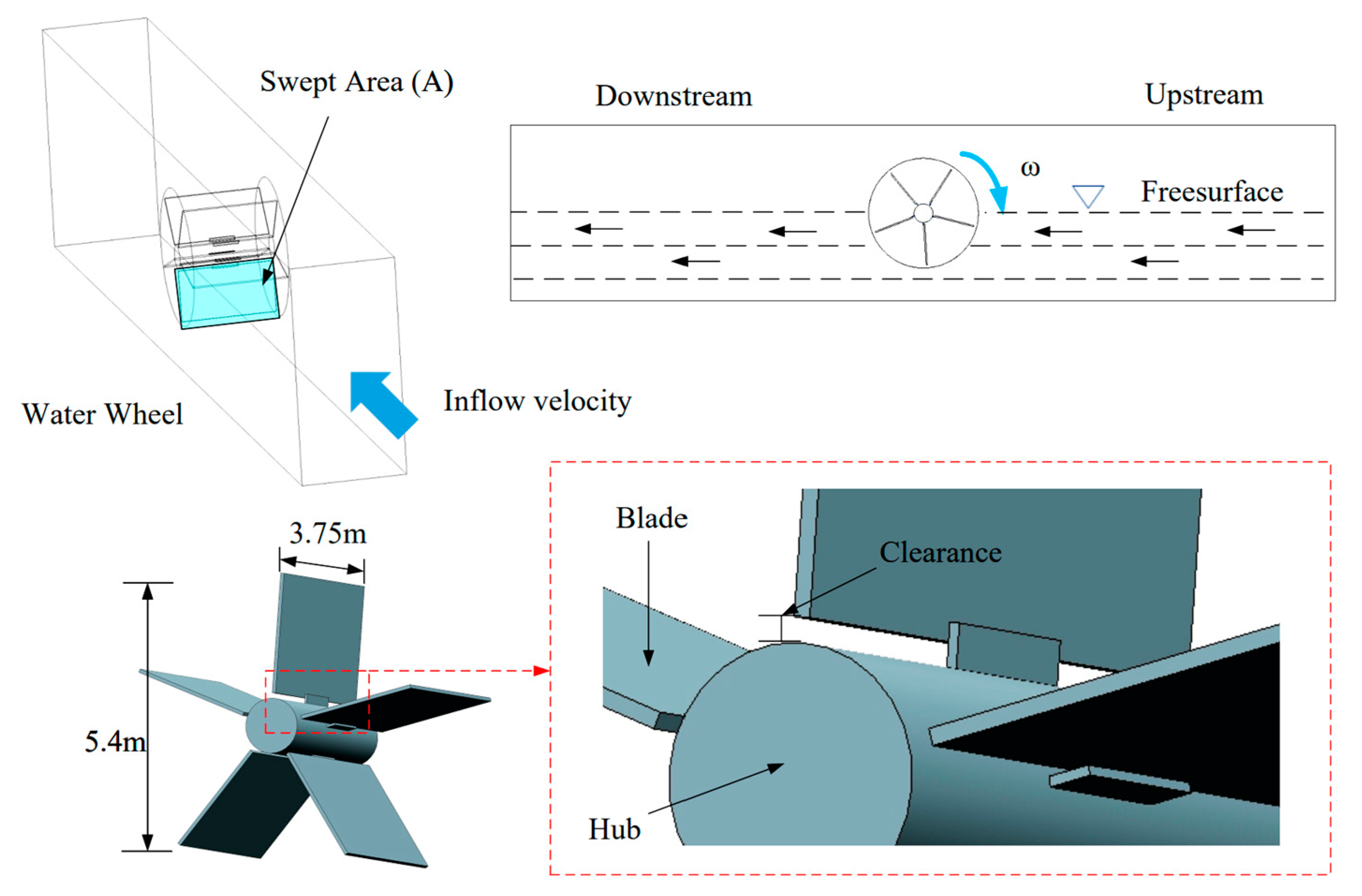
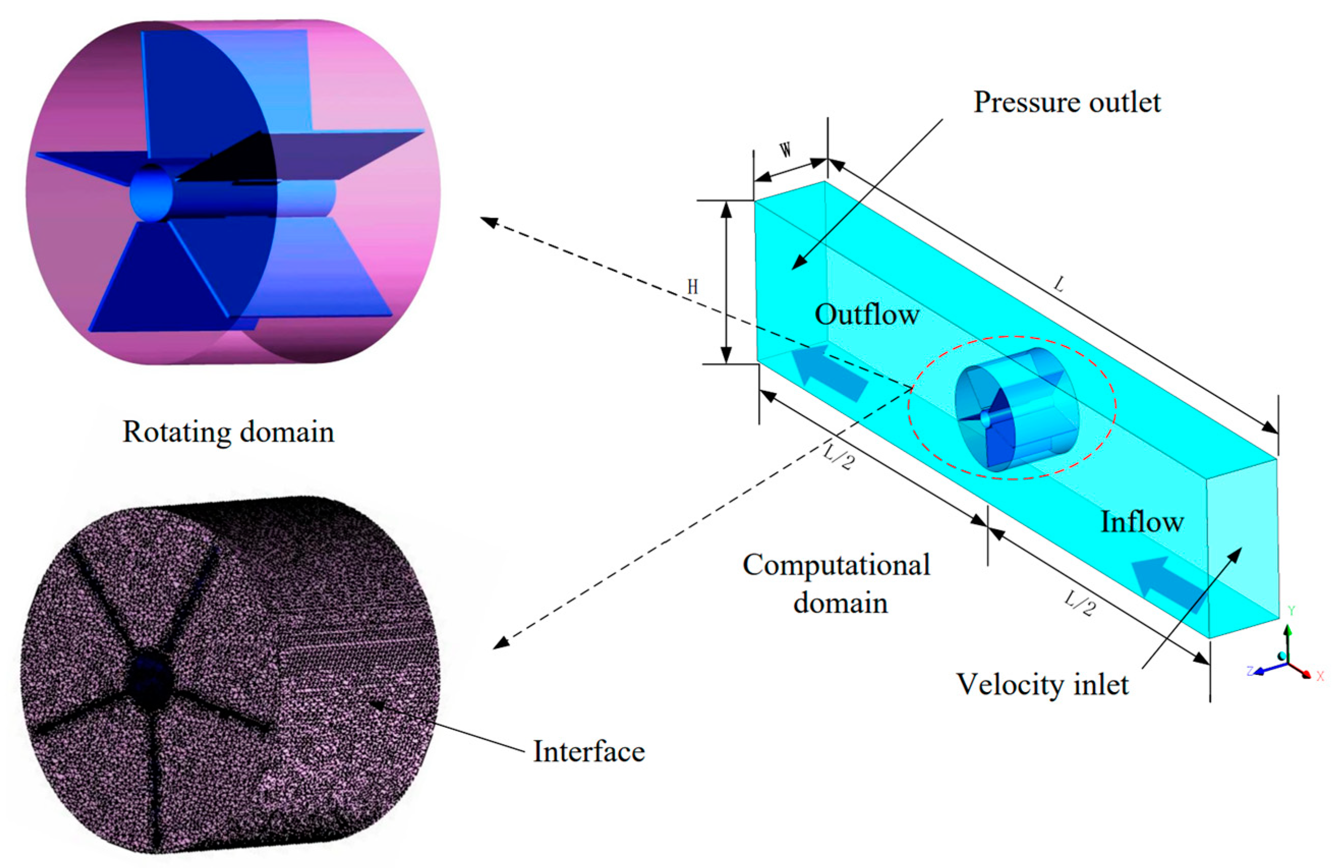
3.1. Computation Domain and Boundary Conditions

The simulation model and operating condition of the water wheel as shown in Figure 1. The simulated channel length is 40.5 m (L), width is 4.15 m (W), and height is 8.64 m (H). The real-size water wheel is a five-blade wheel, in which the blades are all designed to be rectangular in shape with clearance configurations installed between each blade and the hub out from the hub. There are four types of clearances, which are 20 mm, 50 mm, 86 mm, and 120 mm. The outer diameter of the wheel is 5.4 m, the width of the wheel is 3.75 m, and the side clearance is 0.2 m. The water level is equal to the central shaft of the water wheel. There are two parts consisting of the simulation domain: the rotating domain and the stationary domain. The stationary domain and the rotating part represent the domain for the stimulated water channel and turbine blade, respectively. Figure 2 shows the computational domain and boundary conditions. Considering the complexity of the water wheel system, a tetrahedral mesh was applied to the simulation domain [10].

Boundary conditions are set as follows:

(1)

Inlet boundary: the water inlet boundary is set as the velocity inlet. The single variable method is adopted in that the inlet of water flow was set at 4 m/s to simulate the ultra-low head site condition. The direction of the inlet velocity is perpendicular to the inlet, and the turbulence intensity is set to a medium value of 5%. Considering that the water and air interface should be separated, the free surface level is set to the same height as the axis of rotation.

(2)

Outlet boundary: the outlet of water flow is set as the pressure outlet, which value is the same as atmospheric pressure.

(3)

Wall boundary: a no-slip wall is imposed on all other walls except the top of the area, which is set for symmetry [10].

(4)

During the calculation process, the influence of gravity is considered. The unsteady calculation method is used to simulate the gas–liquid two-phase, in which the sliding grid is used in the rotation field to ensure that the wheel rotates at 4 rpm.

3.2. Numerical Method

In this study, each numerical case was carried out utilizing the Ansys Fluent [24]. The VOF method and the standard k-ε turbulence model are utilized to analyze the performance of water wheels as well as the changes in the flow field. The sliding mesh was utilized to simulate the rotational motion of the water wheel. Moreover, the interface was adopted to transfer the momentum as well as the energy between the stationary part and the rotating part. The Pressure Implicit Split Operator scheme is adopted to perform pressure–velocity coupling and the Body Force Weighted scheme is applied to calculate Pressure. The First Order Upwind was utilized to discretize the momentum and turbulent kinetic energy, while the Modified High-Resolution Interface Capturing is utilized to calculate volume fraction. The computational time step was set as 0.06 s and the maximum iteration step in each time step was 15 to obtain the balance between accuracy and efficiency.

3.3. Grid Verification and Validation of Results

For the verification of grid independence, four typical meshes on the 86mm clearance configuration of the water wheel are applied to evaluate the influence of mesh elements quantity, as shown in

Table 1. Mesh independence test.

	Elements (×106)	Averaged Torque (×105 N·m)
Mesh 1	1.26	2.24
Mesh 2	1.46	2.20
Mesh 3	2.43	2.44
Mesh 4	3.01	2.36

. It can be observed that as the mesh elements increases, the averaged torque tends to a stable value. Therefore, Mesh 3 is chosen to conserve computational resources and achieve accurate simulation results.

It is crucial that verify the established model through experiments. Accordingly, an experimental setup was installed in Jiangxi Gongfu Machinery Co. Ltd., Nanchang, China [24]. For the verification of the accuracy of the model used, the experimental setup is shown in Figure 3.

A water wheel with an 86 mm clearance was used in the experiment. The Propeller Flow Velocity Meter in the experiment is the same as in Ref. [24], which measured inlet velocity. The rotor diameter of the instrument is 60 mm, and the variation range of flow velocity is from 0.05–7 m/s, whose accuracy was ±5%. Ten points were selected at the inlet, and the average value of the measured results was taken as the inlet velocity. In the experiment, the blade is fixed by the combination of the upper fulcrum and shaft baffle. In the study, considering the simple structure, the blade is simplified to a fixed steel plate. The distance from the installation position of the unit to the water inlet and from the water outlet are both 19 m. The electric control system of the GBM permanent magnet electric power station control center produced by GBM Gongfu machinery in Jiangxi Province, China, is used to measure the output and speed of the generator. The GBM power station control center has two sets of control models, which are used for the automatic adaptation of optimal speed and manual speed adjustment, respectively.

Two essential parameters to evaluate the performance of the water wheel are torque and power, which were measured [31]:

$$T=F\times r$$

(19)

$$P=T\times \omega$$

(20)

$$\omega =2\pi n/60$$

(21)

with T is the torque of rotation in N·m, F is the force acting on the blade in N, r is the radius of the water wheel in m, P is the power generated by the water wheel in Watts and ω is the angular velocity in rev/s.

Eventually, the geometrical parameters of the tested wheel and the experimental monitoring and simulation results are delineated in

Table 2. Experiment and numerical simulation results in a clearance configuration of 86 mm.

Material	Number of Blades	Flow Velocity (m/s)	Rotational Speed (rpm)	Output in Experiments (KW)	Output in Numerical Result (KW)	Error (%)
Q235 steel	5	1.3	5	0.34	0.35	2.9
			6	0.55	0.57	3.5
			7	0.67	0.69	4.3

. It can be observed that the results of the simulation show good agreement with the experiment data, where the maximum error is less than 5%. It suffers from well-known limitations on the fabrication of machinery as the most source of errors. The model is validated since it can accurately predict the power generated by the water wheel with an acceptable percentage of error.

4. Performance and Flow Characteristics of Water Wheels

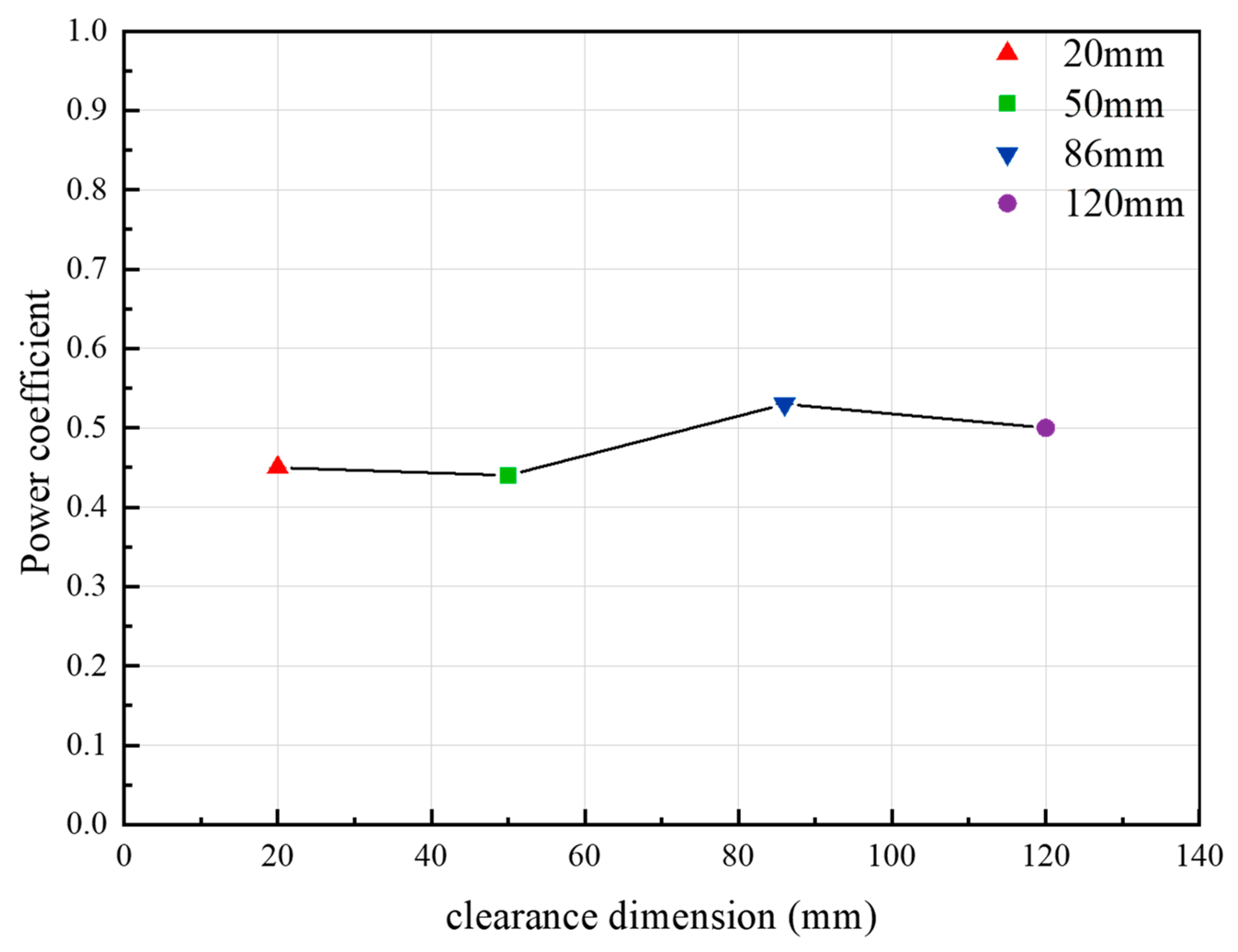
4.1. Water Wheels Performance and Power Fluctuation

To assess how hub clearance affects the water wheel operation, the statistics of the unsteady performances under four different clearance effects are compared. To guarantee the validation and the comparability of operational tests, the rotor is set to constant rotational speed, provided at 4 rpm.

As shown in Figure 4, the torque of each case presents the same tendency in a period. Previously, the torque fluctuation curves change periodically five times within a rotational cycle. Observing that the number of torque change cycles of the four types of water wheels is consistent with the number of blades, which verifies the Ref. [10]. In the clearance configuration, the torque increases up to a maximum of about 70.5° rotation, and then it decreases. It is worth noting that the water wheel with 86 mm clearance has the maximum torque, which indicates the water wheel with appropriate clearance absorbs water energy well. There is little difference between the maximum torque of water wheels with clearance of 20 mm and 50 mm. From the torque curve, the two water wheels operate for a long time under the value of small torque, which means that their output is low and the water wheel is vulnerable to unbalanced torque, resulting in the instability of the unit.

To perform a comprehensive analysis of the ratio of water wheels’ output power to available energy in water, a power coefficient (C_P) was evaluated as [10]:

$$C_p=\frac{T\omega }{\frac{1}{2}\rho A{V}^3}$$

(22)

where ω is the angular velocity, ρ is the density of water, A is the submerged water area of the water wheel, and V is the velocity of the river.

Figure 5 depicts the variation curves of the power coefficient C_p of water wheels under different clearance effects in a cycle. Observing that the water wheel with a clearance of 86 mm showed the optimal performance, with a calculated power coefficient of up to 0.528. This value is successively followed by the water wheels with clearance of 120 mm, 20 mm, and 50 mm, with power coefficients, which are 0.496, 0.445, and 0.441, respectively. The results of the torque curves show merely a slight difference between the water wheels with 20 mm and 50 mm clearances in the ability to capture water energy. The average power coefficient of water wheels, with clearance of 86 mm and 120 mm, proves the result of the torque fluctuation for a rotational cycle that the water wheel with the 86 mm clearance has the best performance. The torque fluctuation of the 86 mm configuration is more stable than the 120 mm one, which means that the efficiency trend is quite constant, and excessive clearance may increase leakage losses.

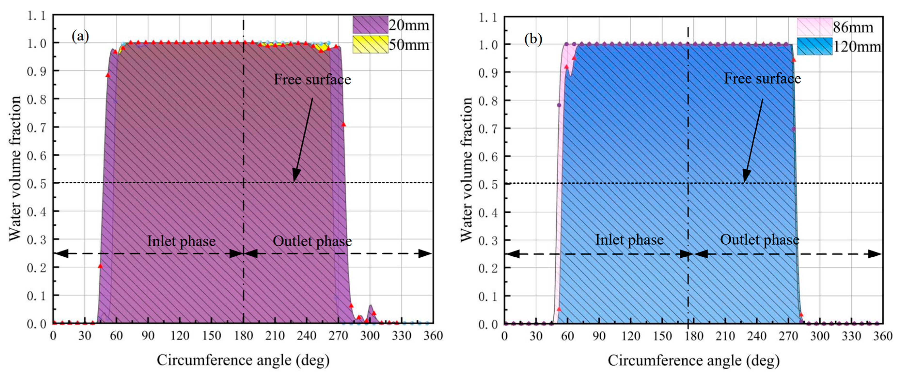
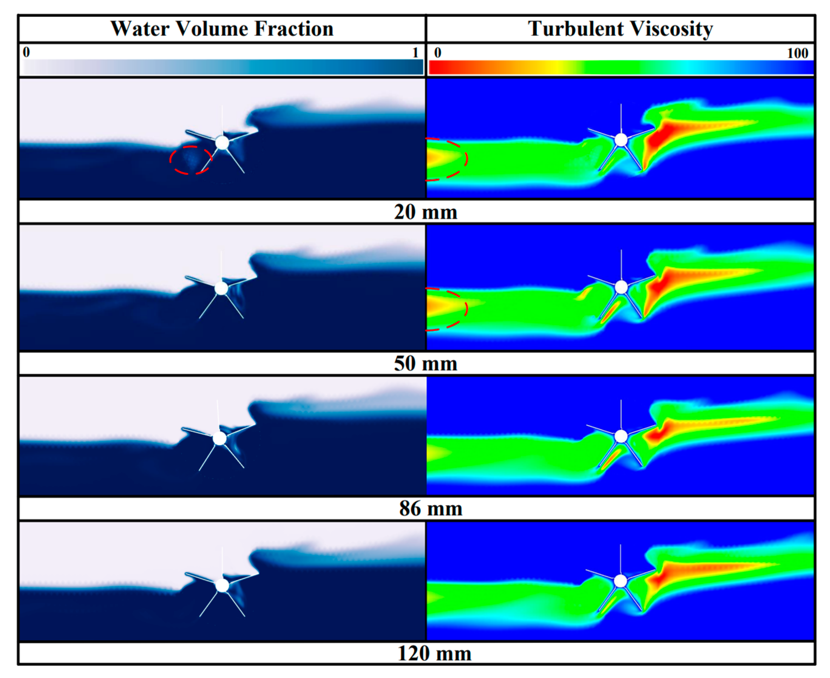
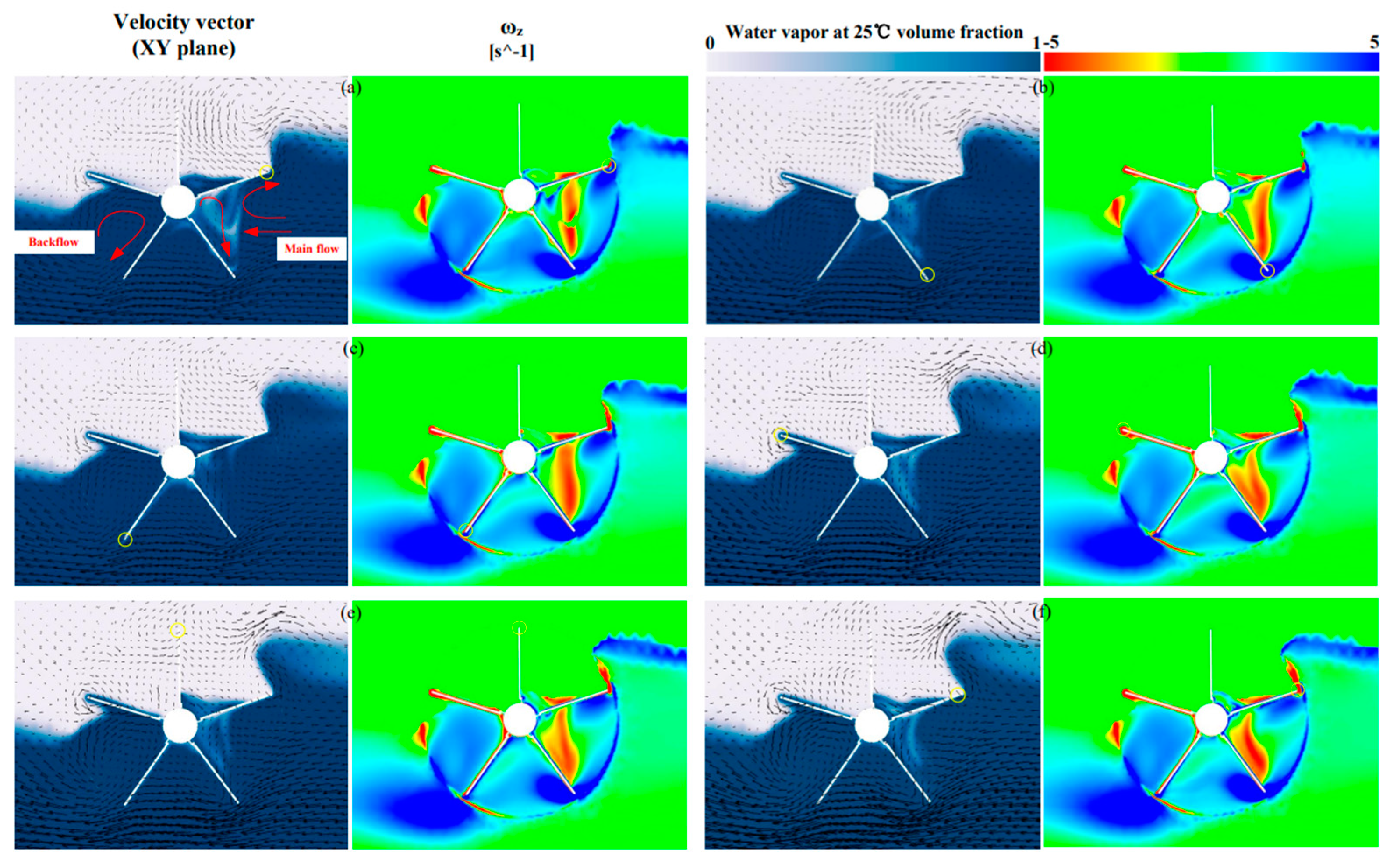
4.2. Analysis of Flow Fields

Since the clearance effects between the blade and hub in a water wheel affect the transfer efficiency of kinetic energy from the flow to the water wheel, it is necessary to analyze the flow field of water wheels to better choose appropriate clearance to improve efficiency in design. Two points are, respectively taken from the center of the width of the water wheel to 2D length in the inlet and outlet directions. The upstream and downstream water depths are measured in these two points, Δd. To better describe the fluctuation of Δd, a non-dimensional parameter Δd_p is defined as:

Δd_p = (Δd_i − Δd_ave)/Δd_ave

(23)

where Δd_i is defined as the torque at each time step. Δd_ave is a time-average depth between the upstream and downstream.

The water level difference and fluctuation between upstream and downstream water wheels under different clearance effects in a cycle are shown in Figure 6a,b. The average difference in the water level reaches the highest in the 86 mm clearance configuration while its fluctuation amplitude is the gentlest, indicating that it can capture the highest water energy and stable operation in the four configurations. Interestingly, the Δd values are elevated considerably at the water wheel with a 20 mm clearance, which is slightly smaller than the 120 mm clearance configuration, and larger than that of the 50 mm clearance configuration. It verifies the previous result that the efficiency and torque of a water wheel with 20 mm clearance are greater than the water wheel with 50 mm clearance. Figure 6b shows that the fluctuation amplitude of clearance 20 mm is significantly larger than the other three types. Therefore, smaller clearances can increase flow complexity and reduce the performance of these water wheels. From an experimental point of view, the larger fluctuation range of upstream and downstream water level difference indicates that the more severe collision between the hub and blade, resulting in complex changes in the flow field, pulse noise signal and vibration, and other adverse problems, and ultimately easily lead to the destruction of the system.

In order to better analyze the different performances of water wheels with different clearance configurations, characteristics of the flow field around the wheel at different circumferential angles (θ) were studied by numerical analysis. Herein, before calculation, a point located in the middle of the width as well as the top of the outer circumference of the water wheel is selected to study. The increased direction of the circumference angle θ is the same as the rotation direction of the rotating domain. Figure 7 illustrates the comparison of time-averaged volume fractions of water at the outer circumference in four configurations. To clearly distinguish the air-water interface and combined with the power coefficient (C_P) of water wheels, the results are divided into two groups of data for comparison, within the water area is α = 1, the air area is α = 0, and α = 0.5 is the air-water interface. Figure 7a shows a comparison between water wheels with 20 mm clearance and 50 mm clearance, and water wheels with 86 mm clearance and 120 mm clearance are demonstrated in Figure 7b.

Significantly, the water wheel with an 86 mm clearance configuration (optimal clearance) occupies the longest water domain, from 61.92° to 208.8°. In addition, the clearance of 120 mm has the second-longest water domain, while the water wheel with a clearance of 20 mm and 50 mm has a similar water area. However, the water wheel with a 20 mm clearance configuration has the considerably longest air–liquid mixing region, as illustrated in Figure 7a. It indicated that a large amount of air enters at its inlet and outlet, owning to the blocking phenomenon and violent fluctuation of the water level difference between the upstream and downstream in the outlet region. Furthermore, by comparing the water volume fraction in Figure 7b, it can be seen that the value of water volume fractions of the clearance of 120 mm fluctuates intensively in the inlet region and only achieves α = 1 until θ = 77.76°.

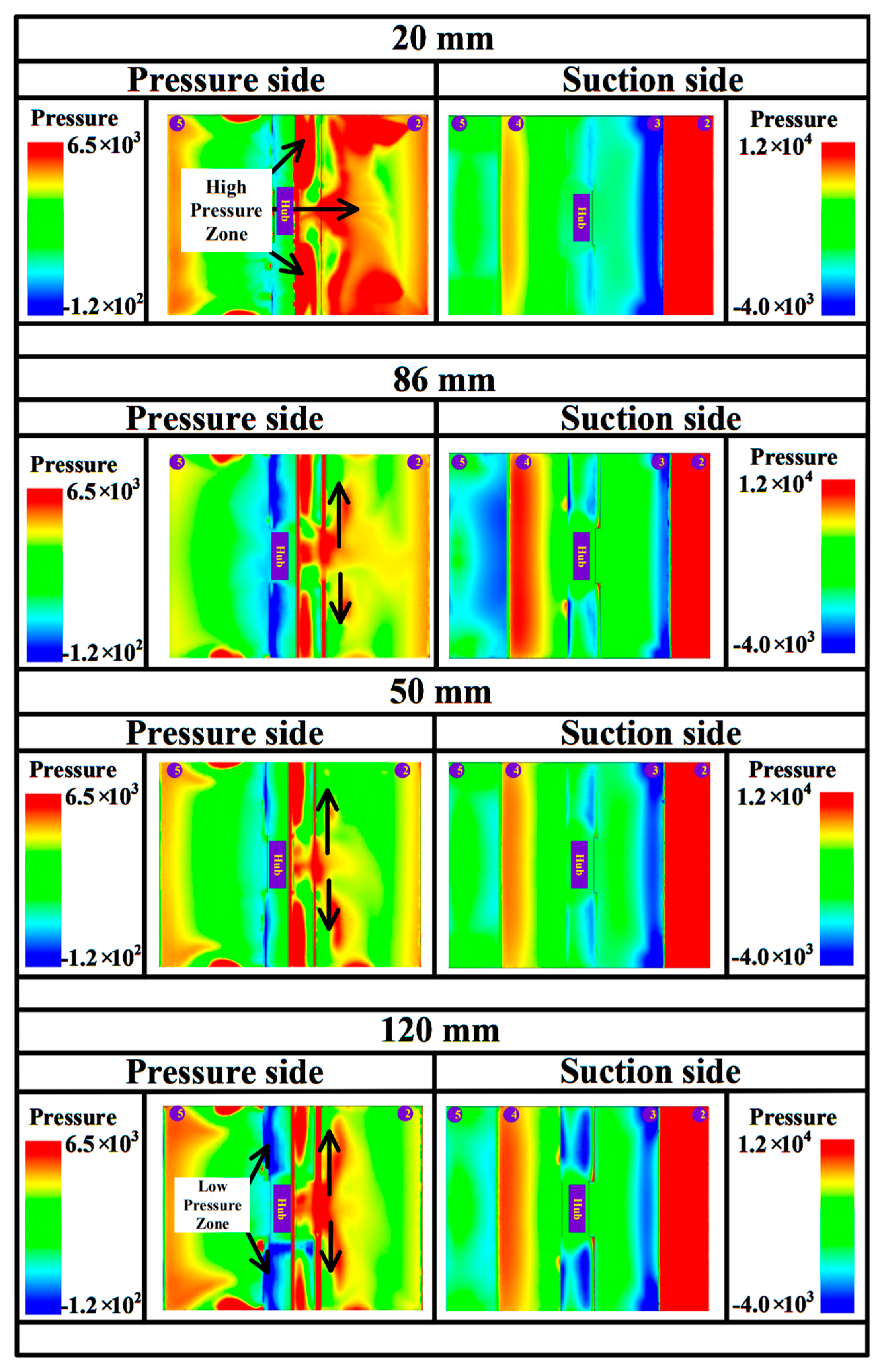
4.3. Energy Dissipation Analysis and Coupling Mechanism of Vorticity-Pressure

The reduction in flow energy dissipation in hydraulic machines is important in improving their energy conversion efficiency [32]. To further study the turbulent characteristics in one cycle of the water wheels, the turbulent viscosity which can characterize the energy dissipation mechanism is introduced.

In Figure 8, a significant amount of air enters the inlet and outlet of the 20 mm clearance water wheel, causing violent turbulent movement in the water flow. This result substantiates that the value of Δd_p of the water wheel with 20 mm clearance fluctuates strongly, as shown in Figure 6, and is consistent with the complicated air–liquid mixing region shown in Figure 7a. Moreover, it can be observed that the outlet exhibits a large number of turbulent viscosity owning to an unsteady flow field under the operation of the 120 mm clearance water wheel. With the clearance enlarged to 50 mm, the turbulent viscosity distributed in the vicinity of the inlet between the left blades decreases; besides, the turbulent viscosity under the hub enhances to the largest during the operation of the water wheel with 50 mm clearance. Further, when the clearance increases to 86 mm, the turbulent viscosity distributed between the left blades abates to the minimum. The 86 mm clearance water wheel has the smallest turbulent viscosity over all the configurations, which presents that the 86 mm clearance water wheel has the steadiest operation flow field and the least energy losses. When the clearance increases to 120 mm, the excessive clearance will let a larger amount of air enters the water, causing unnecessary kinetic energy dissipation.

As can be seen from Figure 6, it is worth noting that water wheels with 20 mm clearance and 120 mm clearance have the largest clearance difference but little difference between upstream and downstream water levels. In comparison to the water wheel with 20 mm clearance, the value, as well as the range of turbulent viscosity of 120 mm clearance, are smaller and narrower. The turbulent viscosity distributed in the outlet has significantly diminished. This result strongly proved that the setting of water wheel clearance can attenuate outcomes of the blocking effect of the river channel and reduce the potential energy loss and kinetic energy dissipation while maintaining high efficiency.

The high hydraulic loss regions are always accompanied by vortices and backflows. To analyze the reason for the energy transport and dissipation of water wheels, the flow field and the distribution of velocity vectors visualized in the XY plane and vorticity in the Z component are delineated in Figure 9 and Figure 10. In an 86 mm clearance water wheel, when the blade marked with yellow circle contacts the water surface, a swirling flow begins to generate. Observing that a vortex is cut off into two parts owning to the main flow and blade tips shows a large number of negative values of vorticity. When the water wheel rotates about θ = 72° in Figure 9b, the vortex attached between the two right blades shows the maximum value while the region is the smallest. The region directly below the hub shows negative vorticity, which shows the minimum scope in the whole period at this time. In Figure 9c, the anti-clockwise vortex is fully developed and occupies a wide range of positive values of vorticity. The negative values of vorticity under the hub start to increase while the clockwise vortex on the left hand of the water wheel remains a large area of negative vorticity. From Figure 9d–f, the anti-clockwise vortex is mostly attached to the right-hand blade submerged in the water. It firstly diminishes in Figure 9e and then increases to the maximum in Figure 9f, which demonstrates a quasi-periodicity of the vortex progress.

For the water wheel with 120 mm clearance, the anti-clockwise vortex is much larger than the 86 mm configuration. In Figure 10a, there are few positive values of vorticity attached to the right-hand blade submerged in the water. It reflects that excessive clearance would cause a more complex flow to consume energy. In Figure 10b, it can be observed that the positive values show a more concentrated distribution. Meanwhile, the vorticity under the hub exhibits the minimum values, which represent the air entering through the clearance into the water causing a chaotic effect. While in Figure 10c, the positive values of vorticity decrease to the minimum in the whole period. Then, the anti-clockwise vortex demonstrates a hollow heart phenomenon, which means the intense flow during the operation of the water wheel. As shown in Figure 10e, the positive values of vorticity represent a twist phenomenon. Due to the blade pushing into the water, a tip vortex is formed on the right-hand blade. At end of the period, the vorticity gradually decreases. Based on the aforementioned analysis, it is found that the exaggerated clearance can induce the flow separation phenomenon and form a large-scale vortex, significantly attenuating the efficiency of the water wheel.

The complexity of the water wheel flow field results in an uneven pressure distribution on blade surfaces. In Figure 11, the pressure distribution of water wheels from bird’s eye views of the pressure side and suction side under different clearance configurations. On the pressure side of the number 2 blade, the high-pressure values are mainly distributed at the hub side of the blades and increase from the middle to both sides. This phenomenon occurs because the remains water crushes into the area between the number 1 blade and the number 2 blade, which will produce flow shock in these regions and further result in the high-pressure zone (HPZ). Furthermore, the HPZ is basically concentrated at the hub corresponding to the clearance region and gradually decreases in the direction of the black arrow. It is noticeable that with the increase in the width of clearance, the HPZ in these regions gradually attenuated, but too large clearance (120 mm) results in uneven pressure distribution of the hub and even a negative pressure phenomenon. As for the suction side of blade surfaces, the HPZ is distributed on the number 2 blade surfaces and the edge of the number 4 blade away from the hub side. Observing that far away from the pressure side of the number 3 blade occurs different levels of low pressure under different clearance effects. Interestingly, the negative pressure scope shows a similar pattern, increasing from the middle of the number 3 blade to both sides in these configurations.

Observing that the 86 mm clearance of the water wheel has the most uniform distribution of pressure, indicating that the more proper the clearance, the more even the pressure distribution is. By setting an appropriate clearance, it can effectively reduce the fatigue damage of the blade and hub caused by water impact, better withstand vibration, and avoid the adverse impact of noise oscillation unit, which is one of the important reasons that the torque and efficiency of other clearance configurations are lower than the optimal clearance configuration. The combined present and future findings might help to find ways to enhance the efficiency and increase the lifespan of water wheels.

5. Characteristics and Distribution of Entropy Production

However, the relationship between vorticity–pressure and irreversible energy loss of water wheels under different clearance effects is still unclear, and needs further discussion. In the existing studies, the energy characteristic of water wheels merely concentrated on the analysis of the flow field, it is urgent to find a new method to directly show the location of energy loss. In addition, the performance of water wheels is closely linked to their energy loss characteristics, hence further investigating the energy loss mechanism of water wheels could contribute to its performance prediction and design of optimal clearance.

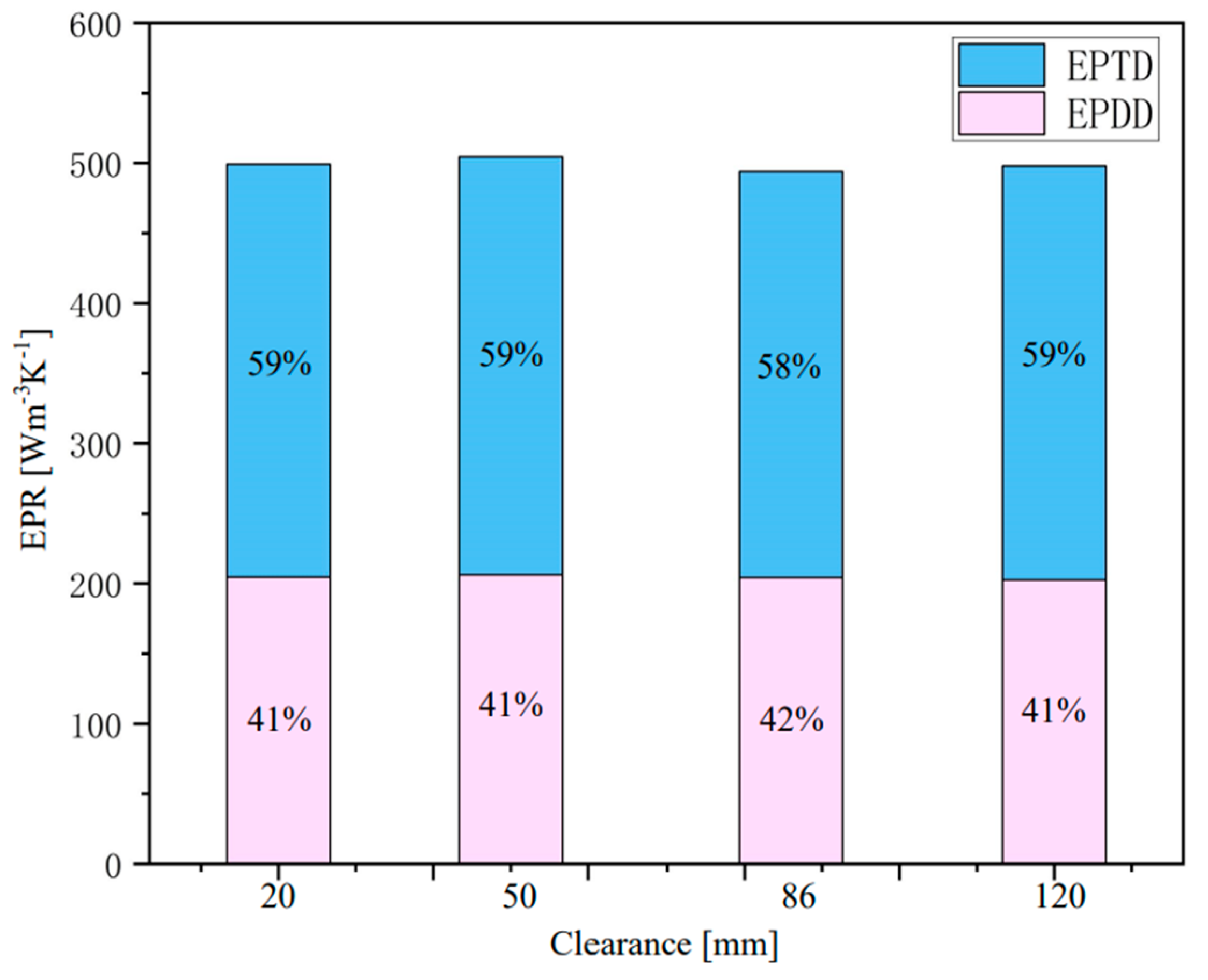
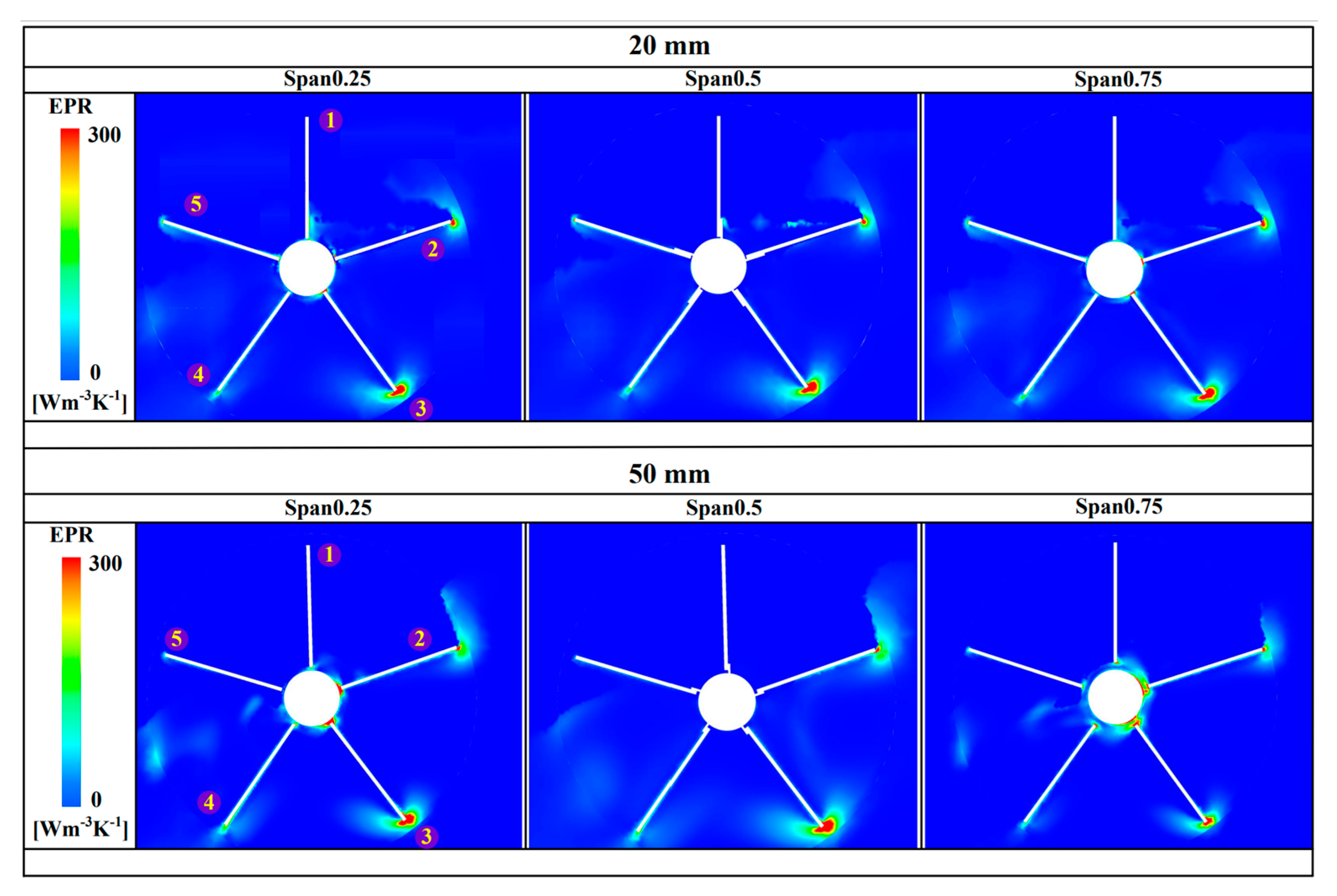
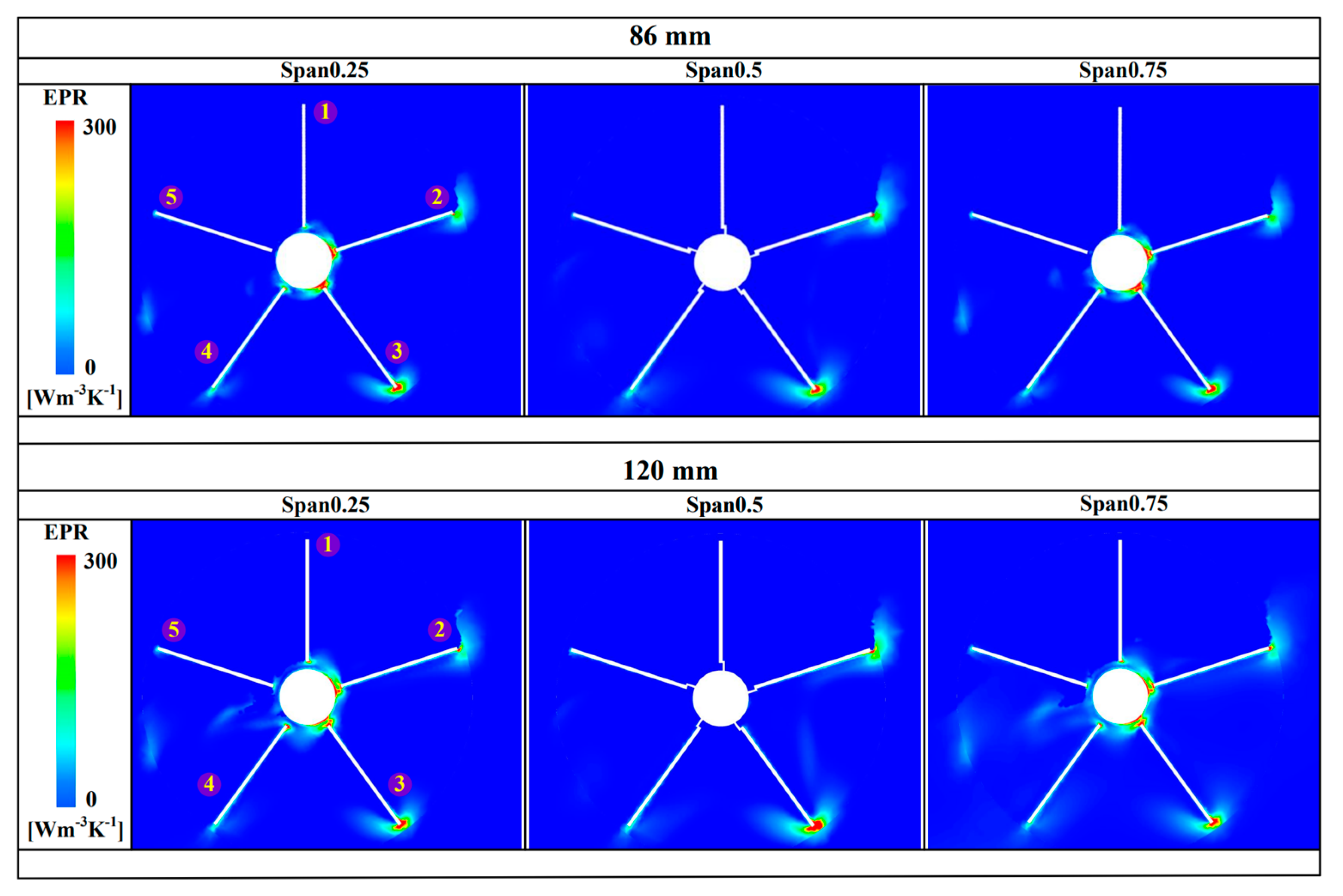
5.1. Distributions of EPR of Water Wheels

To better reveal the value of the entropy production under different clearance configurations of water wheels, the distribution of entropy production is shown in Figure 12. The entropy production is mainly composed of EPR (EPDD and EPTD), while the proportion of EPWS is too small but cannot be ignored, the detail of the distribution of EPWS will be discussed in Section 5.2. It is obvious that the percentage of EPTD is larger than EPDD under four different clearance configurations of water wheels. Moreover, the value of EPR reaches the minimum at 86 mm clearance water wheel while the 50 mm clearance water wheel has the maximum value under the four conditions.

To further reveal the detail of the irreversible energy loss in the water wheels, distributions of EPR (EPDD and EPTD) on the three different sections (span 0.25, span 0.5, and span 0.75) of the water wheels, as shown in Figure 13 and Figure 14. In general, it can be observed that the energy loss is mainly concentrated in the region of the tips of blades submerged in the water due to the flow separation in the tip of the blades. Combined with the low-vorticity region as shown in Figure 9 and Figure 10, it is evident that the flow separation results in the separation vortex and further leads to energy loss and high-value distributions of EPR. Moreover, the regions between blades number 4 and number 5 show a different extent of high EPR distribution under four different clearance configurations, corresponding to the blade wake effect. Owing to the clearance effect, the EPR value of span 0.5 is small than span 0.25 and span 0.75. For the 20 mm clearance water wheel, it can be observed that the small clearance results in the blocking effect occurring between blades number 1 and number 2, further forming the high-level EPR regions. However, for the water wheel with the largest clearance (120 mm), a large number of EPR occur in the clearance between the hub and the blade. It indicates that excessive clearance can also result in unnecessary energy loss.

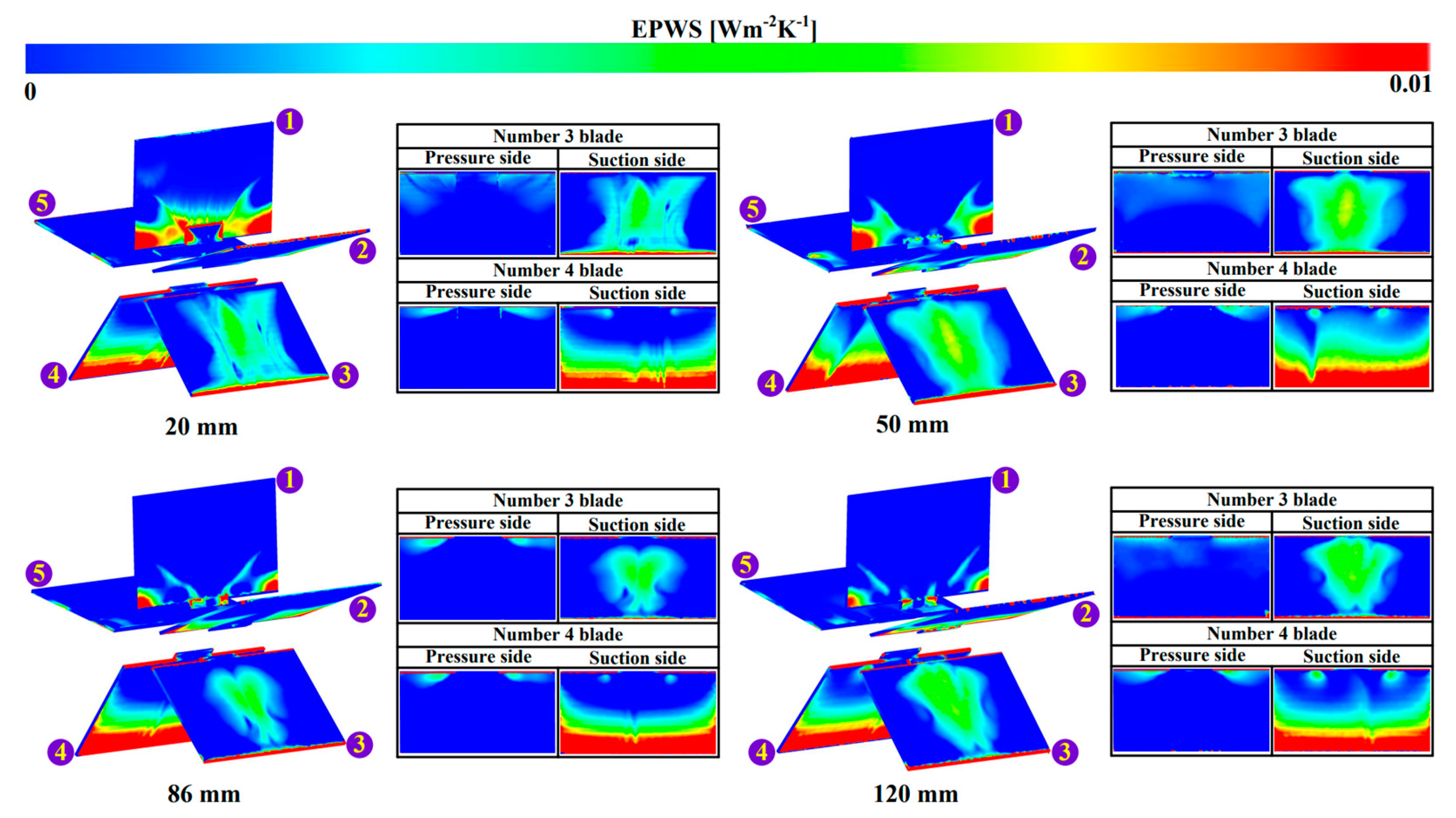
5.2. Distributions of EPWS of Water Wheels

To further investigate the energy loss under different clearances of water wheels, the detailed distribution of EPWS should not be ignored. Figure 15 demonstrates the distribution of EPWS on the hub of water wheels. The maximum EPWS is mainly concentrated on the regions submerged in the water and the areas without settings of clearance, corresponding to the low-pressure region that appears in the hub as shown in Figure 11. The 86 mm clearance water wheel has the most uniform distribution of EPWS in the hub under these four configurations. It is evident that the 86 mm clearance configuration has a better flow regime and reduces energy loss to some extent.

Figure 16 delineates the EPWS distribution of blades under different clearances of water wheels. The overall distribution law of EPWS is similar under different clearances. The maximum EPWS is distributed on the tip region of blades which indicates that the flow separation causes the energy loss. Moreover, the high value of EPWS concentrated on the margin region of the number 1 blade where near the hub, in correspondence to the fluid shock and water-blocking effect. With the setting of appropriate clearance, the EPWS shown in these regions is attenuated. The best distributed EPWS is shown in the water wheel with the 86 mm clearance configuration, indicating that the flow regime near the blade’s wall is well.

Since the situation of the number 3 and number 4 blades is complicated, the detailed distribution of EPWS under different clearance effects is further shown in Figure 15 and Figure 16. Generally, the maximum EPWS is distributed on the suction side of the number 3 and number 4 blades. It is found that the high level of EPWS is shown in the middle of the number 3 blades and decreases to both sides, which corresponds to the high-vorticity region shown in Figure 9 and Figure 10. It is interesting that the maximum EPWS appears on the suction side of the number 3 blade far away from the hub side, corresponding to the low-pressure region shown in Figure 11. This is because the low-pressure region in these areas induced relatively intense velocity and velocity gradients, which result in a large value of EPWS generation [22]. For the suction side of the number 4 blade, it can also find that the maximum value of EPWS is consistent with the maximum distribution of HPZ. Therefore, the coupling mechanism of vorticity–pressure will induce irreversible energy loss in the water wheel while the clearance between blades and hub can affect the performance of water wheels, the appropriate setting of clearance can decrease the irreversible energy loss and improve the efficiency of water wheels.

6. Conclusions

In this research, experimental and numerical simulation methods were used to evaluate the performance and based on the entropy production theory to investigate the energy loss characteristics of the water wheel under different clearance effects. Thus, the following conclusions can be drawn:

• The numerical simulation and experimental results represent a relatively good agreement, with a maximum error of 3.5%.
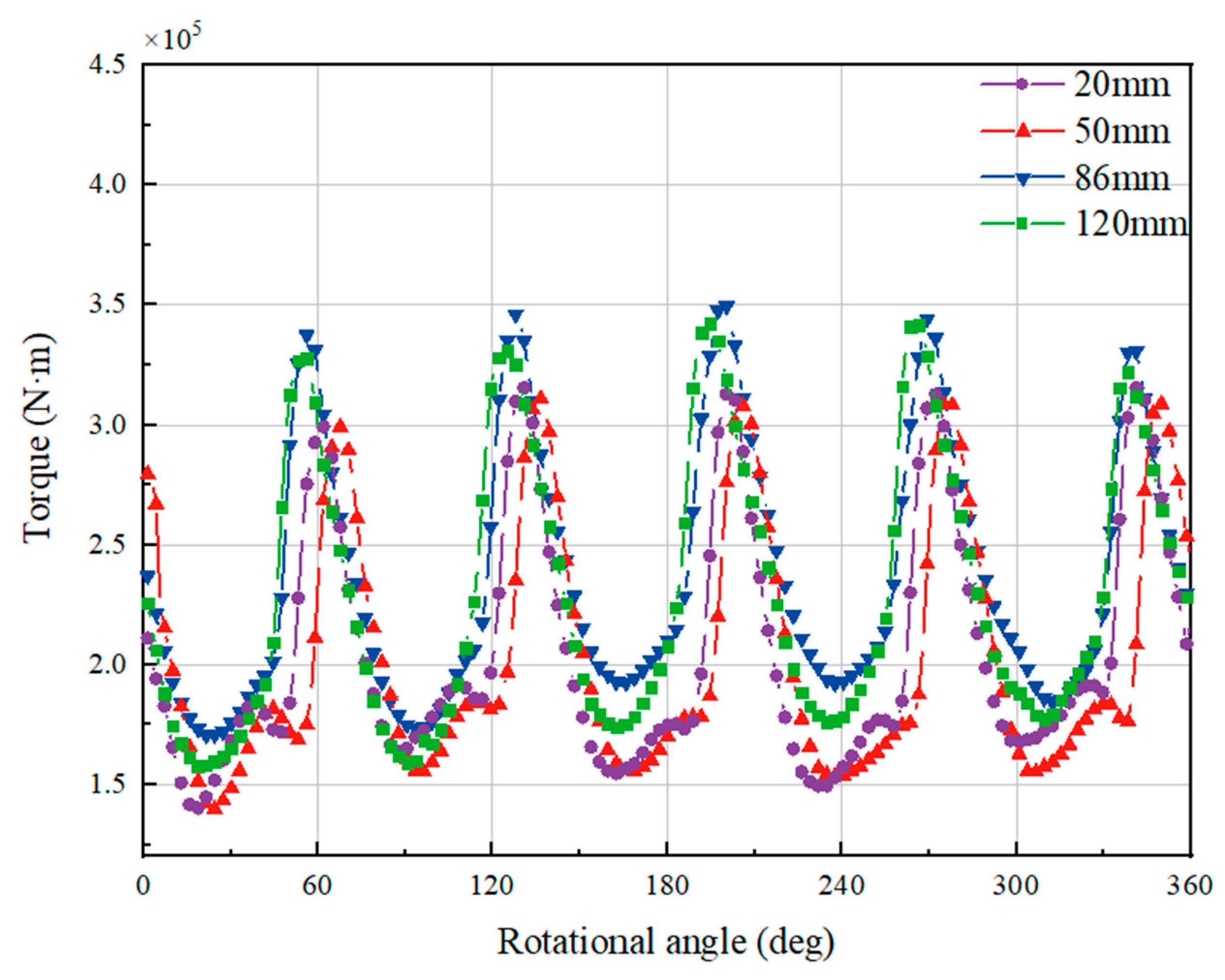
• The torque of the water wheel has periodic transformation within a cycle of rotation, the maximum torque is reached at approximately 70.5° per period. Under the same working conditions, the performance of water wheels can be elevated by 8.7% by setting appropriate clearance.
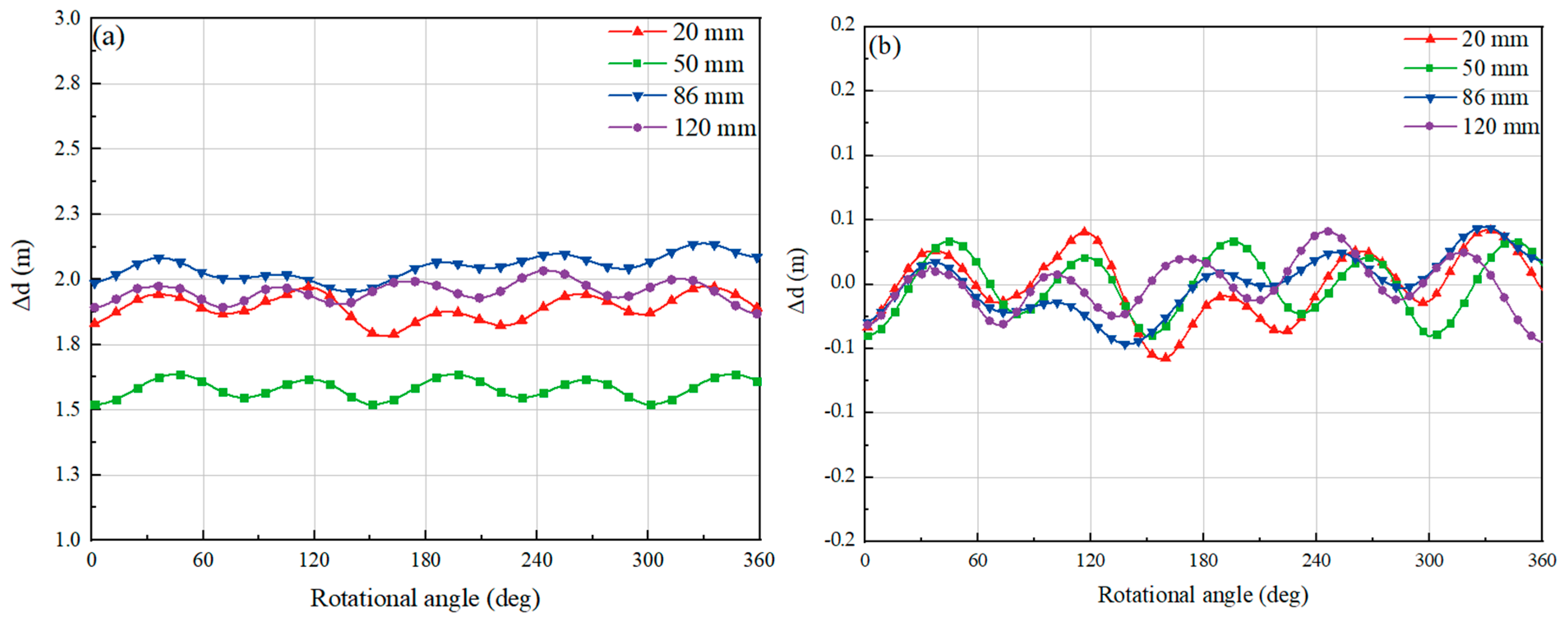
• It was found that the average difference in water level is the highest in the water wheel with the 86 mm clearance configuration, and its fluctuation amplitude is the gentlest. The water wheels with 20 mm clearance and 120 mm clearance have a slight difference in the average difference in water level but the efficiency of maximum clearance (120 mm) is greater than that of minimum clearance (20 mm). The water wheel with optimal clearance can reduce air intruding into the water and attenuate the complexity of the water flow, potentially enhancing the performance of water wheels.
• It proved that the setting of water wheel clearance can attenuate outcomes of the blocking effect of the river channel and reduce the potential energy loss and kinetic energy dissipation while maintaining high efficiency. By comparing the most efficient two configurations of the vortex evolution and pressure distribution, it is illustrated that the optimal clearance can target eliminating vortical flow and improving flow adaptability, avoiding unnecessary energy losses, and decreasing the uneven pressure.
• As a new method, the irreversible energy loss characteristics can be intuitively diagnosed by using the entropy production method in water wheels under different clearance effects. The coupling mechanism of vorticity–pressure which will induce irreversible energy loss of the water wheel under different clearance effects is investigated. Hence, this research can provide a reference for the optimization of clearance between the hub and blade of water wheel performance.

References

1. Cassan, L.; Dellinger, G.; Maussion, P.; Dellinger, N. Hydrostatic Pressure Wheel for Regulation of Open Channel Networks and for the Energy Supply of Isolated Sites. Sustainability 2021, 13, 9532. [Google Scholar] [CrossRef]
2. Bachan, A.; Ghimire, N.; Eisner, J.; Chitrakar, S.; Neopane, H.P. Numerical analysis of low-tech overshot water wheel for off grid purpose. J. Phys. Conf. Ser. 2019, 1266, 012001. [Google Scholar] [CrossRef]
3. Senior, J.; Saenger, N.; Müller, G. New hydropower converters for very low-head differences. J. Hydraul. Res. 2010, 48, 703–714. [Google Scholar] [CrossRef]
4. Quaranta, E.; Revelli, R. Gravity water wheels as a micro hydropower energy source: A review based on historic data, design methods, efficiencies and modern optimizations. Renew. Sustain. Energy Rev. 2018, 97, 414–427. [Google Scholar] [CrossRef]
5. Paudel, S.; Saenger, N. Effect of channel geometry on the performance of the Dethridge water wheel. Renew. Energy 2018, 115, 175–182. [Google Scholar] [CrossRef]
6. Quaranta, E.; Müller, G. Sagebien and Zuppinger water wheels for very low head hydropower applications. J. Hydraul. Res. 2017, 56, 526–536. [Google Scholar] [CrossRef] [Green Version]
7. Ceran, B.; Jurasz, J.; Wróblewski, R.; Guderski, A.; Złotecka, D.; Kaźmierczak, Ł. Impact of the Minimum Head on Low-Head Hydropower Plants Energy Production and Profitability. Energies 2020, 13, 6728. [Google Scholar] [CrossRef]
8. Quaranta, E.; Müller, G. Noise Generation and Acoustic Impact of Free Surface Hydropower Machines: Focus on Water Wheels and Emerging Challenges. Int. J. Environ. Res. Public Health 2021, 18, 13051. [Google Scholar] [CrossRef]
9. Butera, I.; Fontan, S.; Poggi, D.; Quaranta, E.; Revelli, R. Experimental Analysis of Effect of Canal Geometry and Water Levels on Rotary Hydrostatic Pressure Machine. J. Hydraul. Eng. 2020, 146, 04019071. [Google Scholar] [CrossRef]
10. Nguyen, M.H.; Jeong, H.; Yang, C. A study on flow fields and performance of water wheel turbine using experimental and numerical analyses. Sci. China Technol. Sci. 2018, 61, 464–474. [Google Scholar] [CrossRef]
11. Jasa, L.; Priyadi, A.; Purnomo, M.H. Experimental Investigation of Micro-Hydro Waterwheel Models to Determine Optimal Efficiency. Appl. Mech. Mater. 2015, 776, 413–418. [Google Scholar] [CrossRef]
12. Tevata, A.; Inprasit, C. The Effect of Paddle Number and Immersed Radius Ratio on Water Wheel Performance. Energy Procedia 2011, 9, 359–365. [Google Scholar] [CrossRef] [Green Version]
13. Quaranta, E.; Revelli, R. Hydraulic Behavior and Performance of Breastshot Water Wheels for Different Numbers of Blades. J. Hydraul. Eng. 2016, 143, 0401607. [Google Scholar] [CrossRef]
14. Quaranta, E.; Revelli, R. CFD simulations to optimize the blade design of water wheels. Drink. Water Eng. Sci. 2017, 10, 27–32. [Google Scholar] [CrossRef] [Green Version]
15. Quaranta, E.; Revelli, R. Performance Optimization of Overshot Water Wheels at High Rotational Speeds for Hydropower Applications. J. Hydraul. Eng. 2020, 146, 06020011. [Google Scholar] [CrossRef]
16. Warjito, A.D.; Budiarso, P.A. The effect of bucket number on breastshot waterwheel performance. IOP Conf. Ser. Earth Environ. Sci. 2018, 105, 12031. [Google Scholar] [CrossRef]
17. Licari, M.; Benoit, M.; Anselmet, F.; Kocher, V.; Clement, S.B.; Faucheux, P.L. Study of low-head hydrostatic pressure water wheels for harnessing hydropower on small streams. In Proceedings of the Congrès Français de Mécanique, Brest, France, 26–30 August 2019. [Google Scholar]
18. Lin, T.; Li, X.; Zhu, Z.; Xie, J.; Li, Y.; Yang, H. Application of enstrophy dissipation to analyze energy loss in a centrifugal pump as turbine. Renew. Energy 2020, 163, 41–55. [Google Scholar] [CrossRef]
19. Kock, F.; Herwig, H. Local entropy production in turbulent shear flows: A high-Reynolds number model with wall functions. Int. J. Heat Mass Transf. 2004, 47, 2205–2215. [Google Scholar] [CrossRef]
20. Herwig, H.; Fabian, K. Direct and indirect methods of calculating entropy generation rates in turbulent convective heat transfer problems. Heat Mass. Tran. 2006, 43, 207–215. [Google Scholar] [CrossRef]
21. Duan, L.; Wu, X.; Ji, Z.; Xiong, Z.; Zhuang, J. The flow pattern and entropy generation in an axial inlet cyclone with reflux cone and gaps in the vortex finder. Powder Technol. 2016, 303, 192–202. [Google Scholar] [CrossRef]
22. Yu, A.; Tang, Q.; Zhou, D. Entropy production analysis in thermodynamic cavitating flow with the consideration of local compressibility. Int. J. Heat Mass Transf. 2020, 153, 119604. [Google Scholar] [CrossRef]
23. Yu, A.; Tang, Q.; Chen, H.; Zhou, D. Investigations of the thermodynamic entropy evaluation in a hydraulic turbine under various operating conditions. Renew. Energy 2021, 180, 1026–1043. [Google Scholar] [CrossRef]
24. Zhao, M.; Zheng, Y.; Yang, C.; Zhang, Y.; Tang, Q. Performance Investigation of the Immersed Depth Effects on a Water Wheel Using Experimental and Numerical Analyses. Water 2020, 12, 982. [Google Scholar] [CrossRef] [Green Version]
25. Acharyax, N.; Kim, C.G.; Thapa, B.; Lee, Y.H. Numerical analysis and performance enhancement of a cross-flow hydro turbine. Renew. Energy 2015, 80, 819–826. [Google Scholar] [CrossRef]
26. Zhong, H.Z. Fluid’s Engineering Simulation Examples and Applications of Fluent; Beijing Institute of Technology Press: Beijing, China, 2004; ISBN 7564026049. (In Chinese) [Google Scholar]
27. Setyawan, E.Y.; Djiwo, S.; Praswanto, D.H.; Suwandono, P.; Siagian, P.; Naibaho, W. Simulation model of vertical water wheel performance flow. IOP Conf. Ser. Mater. Sci. Eng. 2020, 725, 012020. [Google Scholar] [CrossRef]
28. Adanta, D.; Muhammad, N.; Rizwanul, F.I.M. Comparison of standard k-ε and sst k-ωturbulence model for breastshot waterwheel simulation. J. Mech. Sci. Eng. 2020, 7, 39–44. [Google Scholar] [CrossRef]
29. Launder, B.E.; Spalding, D.B. The Numerical Computation of Turbulent Flows. Comput. Methods Appl. Mech. Eng. 1974, 3, 2269–2289. [Google Scholar] [CrossRef]
30. Li, D.; Wang, H.; Qin, Y.; Han, L.; Wei, X.; Qin, D. Entropy production analysis of hysteresis characteristic of a pump-turbine model. Energy Convers. Manag. 2017, 149, 175–191. [Google Scholar] [CrossRef]
31. Yah, N.F.; Oumer, A.N.; Aziz, A.A.; Sahat, I.M. Numerical investigation on effect of blade shape for stream water wheel performance. IOP Conf. Ser. Mater. Sci. Eng. 2018, 342, 012066. [Google Scholar] [CrossRef]
32. Tao, R.; Wang, Z. Comparative numerical studies for the flow energy dissipation features in a pump-turbine in pump mode and turbine mode. J. Energy Storage 2021, 41, 102835. [Google Scholar] [CrossRef]
Figure 1. Geometric model and operating condition of the water wheel.
Water 14 03640 g001
Figure 2. Computational domain and boundary conditions.
Water 14 03640 g002
Figure 3. The five-blade water wheel model was used in experiments.
Water 14 03640 g003
Figure 4. Torque variation of four different clearance scales in a cycle.
Water 14 03640 g004
Figure 5. Comparison of efficiency among different clearance dimensions.
Water 14 03640 g005
Figure 6. Difference in water level, Δd in a cycle (a); Difference in non-dimensional parameter Δdp in a cycle (b).
Water 14 03640 g006
Figure 7. Water volume fractions at the wheel’s outer circumference. (a) Between the clearance of 20 mm and 50 mm; (b) Between the clearance of 86 mm and 120 mm.
Water 14 03640 g007
Figure 8. Profiles of water volume fraction and turbulent viscosity of water wheels under different clearance effects at circumferential angle θ = 288°.
Water 14 03640 g008
Figure 9. Contours of velocity vectors, water volume fraction, and vorticity in a cycle of the 86 mm clearance water wheel. (a) The circumferential angle θ = 0°; (b) The circumferential angle θ = 72°; (c) The circumferential angle θ = 144°; (d) The circumferential angle θ = 216°; (e) The circumferential angle θ = 288°; (f) The circumferential angle θ = 360°.
Water 14 03640 g009
Figure 10. Contours of velocity vectors, water volume fraction, and vorticity in a cycle of the 120 mm clearance water wheel. (a) The circumferential angle θ = 0°; (b) The circumferential angle θ = 72°; (c) The circumferential angle θ = 144°; (d) The circumferential angle θ = 216°; (e) The circumferential angle θ = 288°; (f) The circumferential angle θ = 360°.
Water 14 03640 g010
Figure 11. Pressure distribution on water wheels from bird’s eye views of the pressure side and suction side under different clearance configurations.
Water 14 03640 g011
Figure 12. Distribution of EPR under different clearance configurations.
Water 14 03640 g012
Figure 13. Distribution of EPR in the midsection of water wheels under 20 mm and 50 mm clearances.
Water 14 03640 g013
Figure 14. Distribution of EPR in the midsection of water wheels under 86 mm and 120 mm clearances.
Water 14 03640 g014
Figure 15. Distribution of EPWS in the hub of water wheels under different clearance configurations.
Water 14 03640 g015
Figure 16. Distribution of EPWS in the blades of water wheels under different clearance configurations.
Water 14 03640 g016