Organic Contamination Distribution Constrained with Induced Polarization at a Waste Disposal Site

Abstract

Waste disposal sites are a serious concern due to their potential contamination threat. Site characterizations are the basis for contamination remediation, among which borehole-based methods are time-consuming. This study aims to utilize time-domain induced polarization (TDIP) to constrain groundwater and soil organic contamination. Fourteen TDIP profiles were arranged using three acquisition methods at a disposal site contaminated with benzene. A data quality analysis was first conducted to overcome poor signals in high-salinity groundwater conditions. The TDIP results show that solid waste can be classified into two distinct types based on chargeability. The results of induced polarization measurements and X-ray fluorescence analysis proved the presence of metal substances causing high chargeability. The waste with metals was the benzene contamination source. Finally, we propose a procedure for the integration of geophysical and geochemical methods to delineate contaminated areas. A new roll-along survey protocol was developed to meet the needs of long-profile surveys of contaminated shallow groundwater and soil sites.

1. Introduction

Groundwater contamination caused by waste disposal sites is a serious concern. Contamination related to waste disposal is due to the presence of inorganic substances, organic contaminants and heavy metals in solid wastes [1]. The contaminants penetrate native geological layers because most disposal sites were constructed without an impermeable system underneath [2,3,4], especially in the suburbs of developing countries, where most waste disposal sites are unauthorized [5,6]. Ecosystems and public health are under serious threat after these contaminants enter aquifer systems [7,8]. As a result, organic contamination may cause serious health issues, such as liver, eye, skin and neurological diseases [9,10].

The investigation of contaminated groundwater and soil sites is the basis for remediation [11], which can provide essential information so that the source and the resultant plume can be delineated and remediation areas can be constrained [12,13,14]. Drilling techniques based on sample analysis are the most direct and common means and can accurately acquire the types and concentrations of contaminants [15]. However, there are drawbacks to the application of drilling techniques, such as high costs and time-consuming operations for drilling and the chemical analysis of samples, discontinuous underground information between the boreholes and the risk of contaminants spreading vertically during the drilling process [16,17].

Geophysical methods have recently been increasingly applied for the detection and monitoring of contaminated sites in the field because of their high efficiency, low cost, continuous underground information, and fast data acquisition and processing [18,19], especially for electrical resistivity tomography (ERT) [20]. The induced polarization (IP) method is an extension of the electrical resistivity method, and it can reduce the uncertainty of resistivity results. The IP response can be measured in the time domain (TDIP) and frequency domain (FDIP), and TDIP is often used for field surveys because of the shorter data acquisition time. The TDIP method has been used to characterize groundwater and soil contaminant distributions in landfills [21,22,23], organic-contaminated sites [24,25,26], heavy-metal-contaminated sites [27], etc. In addition, TDIP has also been applied in a large number of waste disposal sites’ delineation, including the characterization of contaminants [1,28,29], the characterization of waste mass [30,31,32] and geological delineation [33].

The TDIP method measures the decay of the secondary voltage after the current is shut off in the underground medium. Unlike the primary voltage measured by ERT, the secondary voltage is more vulnerable to electromagnetic coupling [34] and electrode polarization [35]. In addition, the secondary voltage is low in magnitude, and thus, the data quality is vulnerable to ambient noise [36], especially in sites with high groundwater salinity. Data acquired with a high signal-to-noise ratio (SNR) are the basis for the effective utilization of the IP signal in contaminated sites, and therefore, many studies on data acquisition methods have been conducted [37,38,39].

In general, the interpretation of IP data in waste disposal sites needs to establish a correlation between contamination and IP parameters [23]. Therefore, raw data were processed by de-noising, drift correction [40] and manual removal [41] and were inverted by a full-decay inversion model [42]. Furthermore, laboratory FDIP data for samples were used to aid the TDIP interpretation in contaminated sites because of the rich spectral information [43,44].

In this study, we have characterized a waste disposal site contaminated with benzene using the TDIP method. Three data acquisition methods were tested to ascertain a reliable IP data acquisition method in a high groundwater salinity site. In addition, a laboratory analysis of soil samples was conducted to verify the field results. A link between conductivity from a field survey and that from laboratory measurements was derived. The contamination source was indirectly constrained by the difference in chargeability. Finally, we summarized the procedure for the integration of geophysical and geochemical methods to characterize contaminated areas. A new roll-along measurement method was developed to meet the needs of long and shallow contaminated profile surveys.

2. Materials and Methods

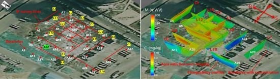
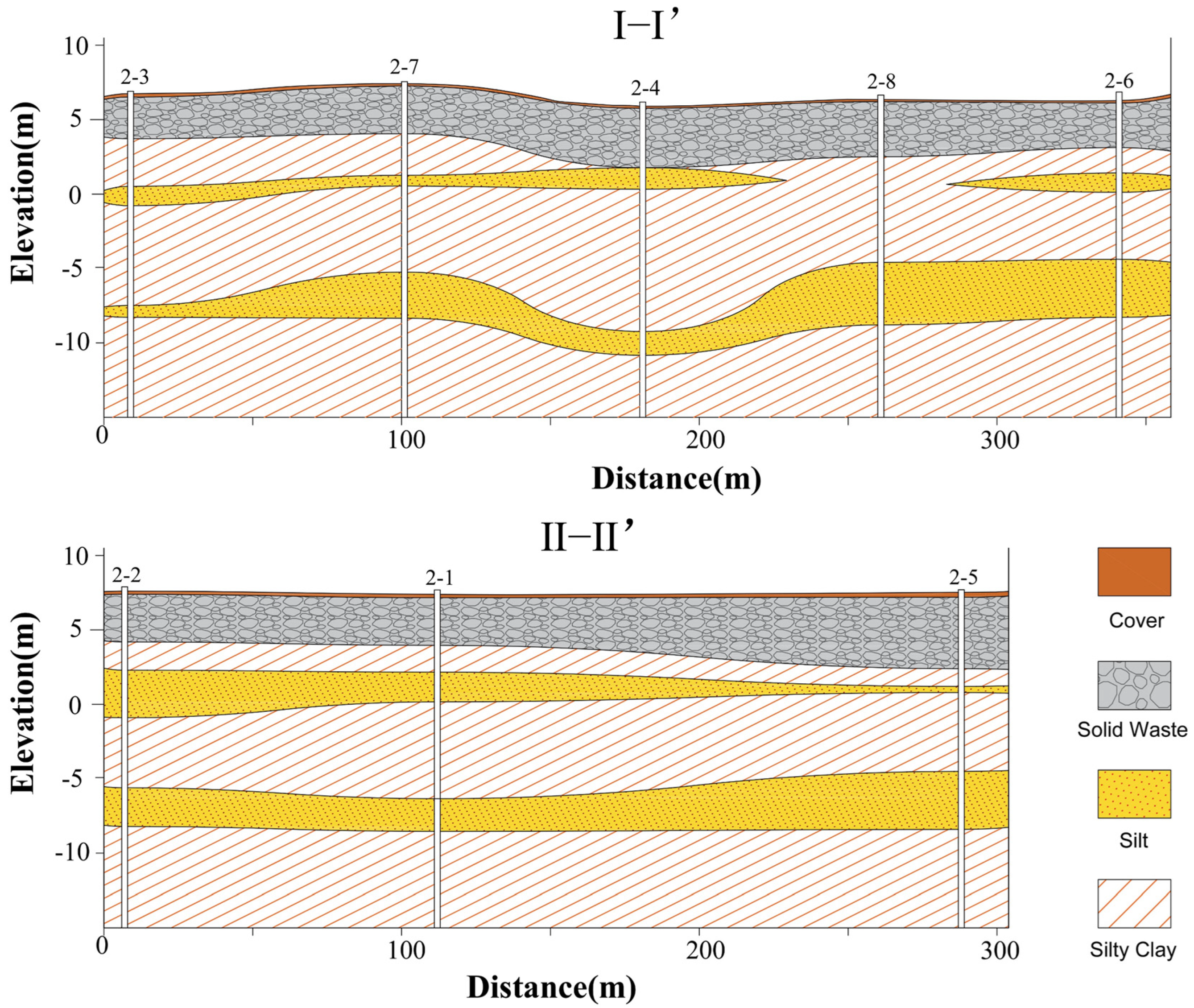
2.1. Site Description

The waste disposal site in this research is situated in the center of Shandong Province, China. A satellite image of this site is shown in Figure 1. This area was woodland before it was landfilled with solid waste. Industrial solid wastes, mainly including salt mud, white mud, coal fly ash and desulfurization gypsum, gradually emerged in this region from 2008 to 2014. The waste deposit takes up around two-thirds of the area, which is approximately 93,400 m². Benzene contamination was distributed in the area above 5 m below the ground surface in the eastern part of the site, but a detailed investigation was required to characterize the benzene contamination source and the resultant plume.

Hydrogeological investigations were carried out between October 2019 and February 2021. Two hydrogeological profiles were located in the north and south of the survey area (Figure 1), and the results are shown in Figure 2. The solid waste overlies native silt and silty clay sediments. The thickness of solid wastes at the site varies from 2.8 to 4.8 m. Hydraulic conductivity values are in the order of 3.75 × 10⁻⁸ m/s for silty clay and 3 × 10⁻⁷ m/s for silt. A low-permeability silty clay layer and silt layer limit the vertical downward migration of contaminants, resulting in the distribution of contamination in a solid waste layer rather than native sediment layers. The direction of groundwater flow is from north to south, with a low hydraulic gradient of 2.5‰. The water table is 5.5 m below the ground surface in the dry season and 5 m in the rainy season. Therefore, the contaminants mainly exist in the unsaturated zone above the water table and hardly migrate horizontally with groundwater.

2.2. Field Time-Domain Induced Polarization Survey

In November 2021, fourteen TDIP profiles were surveyed around the eastern part of the site (Figure 1), where the benzene concentration was high. The existence of solid wastes and the high TDS of groundwater (4677–29,860 mg/L) caused low background resistivity. Acquiring reliable IP data is challenging in such a high groundwater salinity site due to weak second voltage signals [34,35].

The capacitive/inductive coupling and electrode polarization can be reduced by separating the current and potential cables and using non-polarization electrodes [38]. Therefore, three different TDIP data acquisition methods can be used: the standard single-cable layout, separating current and potential cables with stainless steel electrodes, and separating current and potential cables with stainless steel current electrodes and non-polarization potential electrodes. The above three data acquisition methods were tested in profile L1 to ascertain which one was the best choice in the high groundwater salinity site before the whole TDIP survey.

All data profiles were acquired with 32 electrodes spaced 2 m apart with a total length of 62 m. One cable with 32 stainless steel electrodes was used in all profiles for the standard single-cable layout. Two parallel cables shifted by 0.5 m relative to each other gave a total layout of 64 electrodes for double-spread cable layouts. There were 32 stainless steel electrodes used as current electrodes and 32 Pb-PbCl₂ electrodes used as potential electrodes in all profiles, while stainless steel electrodes were used throughout the current and potential cables only in profile L1 to evaluate the data quality of different acquisition methods.

The ABEM Terrameter LS2 was used to obtain TDIP data with a 100 percent duty-cycle. The current was injected in cycles of 4 s, and the voltage decays were recorded in 12 time gates, approximately log-sampled with a time range from 20 ms to 3960 ms (

Table 1. Available apparent chargeability data quantity of TDIP field survey.

IP Gate	Off Time (ms)	Separating Current and Potential Cables		Single Cable
		Stainless Steel Current Electrodes and Non-Polarized Potential Electrodes	Stainless Steel Current and Potential Electrodes
Gate 1	20	204	21	39
Gate 2	60	280	91	88
Gate 3	120	289	146	152
Gate 4	200	293	151	165
Gate 5	300	293	161	173
Gate 6	440	293	162	178
Gate 7	620	293	165	175
Gate 8	880	293	162	175
Gate 9	1280	289	162	172
Gate 10	1880	284	151	168
Gate 11	2760	270	143	157
Gate 12	3960	75	85	52
Total		3156	1600	1694

). Meanwhile, full waveform data of 1000 Hz were collected during measurement. Before measuring TDIP data, the electrodes were wetted with water to diminish the contact resistance and consequently induce capacitive coupling. The multiple-gradient array protocol with 294 quadrupole data points was used for the data acquisition because of its low geometrical factor. Furthermore, the multiple-gradient protocol was modified by recoding the spread file and protocol file to add extra cable and separate current and potential cables to match double-cable layouts.

The TDIP data were manually diagnosed and inverted using Aarhus Workbench [45]. Firstly, apparent resistivity data and the corresponding decay curves were removed when they were negative or had a severely disturbed appearance. Afterward, each gate of the TDIP decay curves was manually inspected. When apparent chargeability decay curves were negative, non-decaying, or overly slow or steep in their decay, they were eliminated. The purpose was to ensure that each decay curve can be reasonably fitted with Cole–Cole model. Finally, the retained data were inverted using full-wave inversion method, obtaining the distributions of resistivity, chargeability, relaxation time and the Cole–Cole exponent [42].

2.3. Soil Sampling and Processing

Soil sample boreholes were drilled immediately after the TDIP survey (Figure 1). A total of 196 soil samples were collected in 29 boreholes at depths of 0.5 to 8 m. In order to delineate the contamination source and plume, 189 soil samples were analyzed for 64 organic contamination indexes, including 2-butanone, benzene, methylbenzene, ethylbenzene, methyl chloride, chlorobenzene, naphthalene, etc. In addition, the conductivity of all soil samples was determined by measuring the conductivity of the extract solution of dried soil according to Soil quality—determination of conductivity—Electrode method (Ministry of Environmental Protection of the People’s Republic of China, HJ 802-2016). Naturally dried soil samples were added to water at a ratio of 1:5 and extracted at 20 °C. The conductivity of the extract solution was determined at 25 °C.

Chemical data were collected by XRF analysis for samples at a depth of 2.5 m from boreholes A12 and A14. The samples were solid wastes. A Thermo Scientific Niton XL3t 960 GOLDD+ handheld X-ray fluorescence analyzer (Thermo Fisher Scientific, Waltham, MA USA) mounted in the National Engineering Laboratory for Site Remediation Technologies in Beijing was used. Each homogenized sample was subjected to a 90 s analysis routine.

2.4. Laboratory Frequency-Domain Induced Polarization Measurement

Laboratory FDIP measurement was conducted to verify the field TD results and aid the TDIP interpretation because of the rich spectral information [43,44]. Samples for the laboratory FDIP column test were collected for two soil samples in the aforementioned XRF analysis. All samples were dried at 180 °C for 10 h and then were saturated using NaCl solution. The conductivity of the solution was 1000 and 10,000 μS/cm according to the TDS of field groundwater.

FDIP spectra were measured for each sample using an Ontash PSIP instrument from Ontash & Ermac, Inc. River Edge, NJ, USA (www.ontash.com). The measurement data included 25 current frequencies between 0.01 and 10,000 Hz that were spread logarithmically. A sinusoidal signal with a 5 V maximum amplitude was used on the current electrodes and a resistor with a 1 kΩ reference. The impedance of the samples was measured, and the complex resistivity was acquired by multiplying the magnitude of the impedance by the geometric factor. The acquired parameters are the magnitude of complex resistivity and phase shifts (phase) of the received potential sinusoid:

$${\rho }^{*}=\left|\rho \right|e^{i\phi },$$

where ${\rho }^{*}$ is the complex resistivity, $\left|\rho \right|$ is the resistivity magnitude and $\phi$ is the phase. The measured phase data were corrected to remove the errors from interactions between the parasitic capacitive coupling and the sample holder at a high frequency according to the model of Wang and Slater [46]. In order to enable a comparison with TDIP survey results, Cole–Cole parameters at the same location as the laboratory samples were extracted and interpolated from field TDIP inversion profiles. The complex resistivity from the field TDIP survey can be computed by the following equation [47,48]:

$${\rho }^{*}\left(\omega \right)={\rho }_0\left[1-m\left(1-\frac{1}{1+{\left(i\omega \tau \right)}^c}\right)\right]$$

where ${\rho }_0$ is the low-frequency resistivity, $m$ is the intrinsic chargeability, $\tau$ is the relaxation time and $c$ is the Cole–Cole exponent. In addition, the laboratory data were fitted using the Cole–Cole model, and the four parameters above were inverted.

3. Results

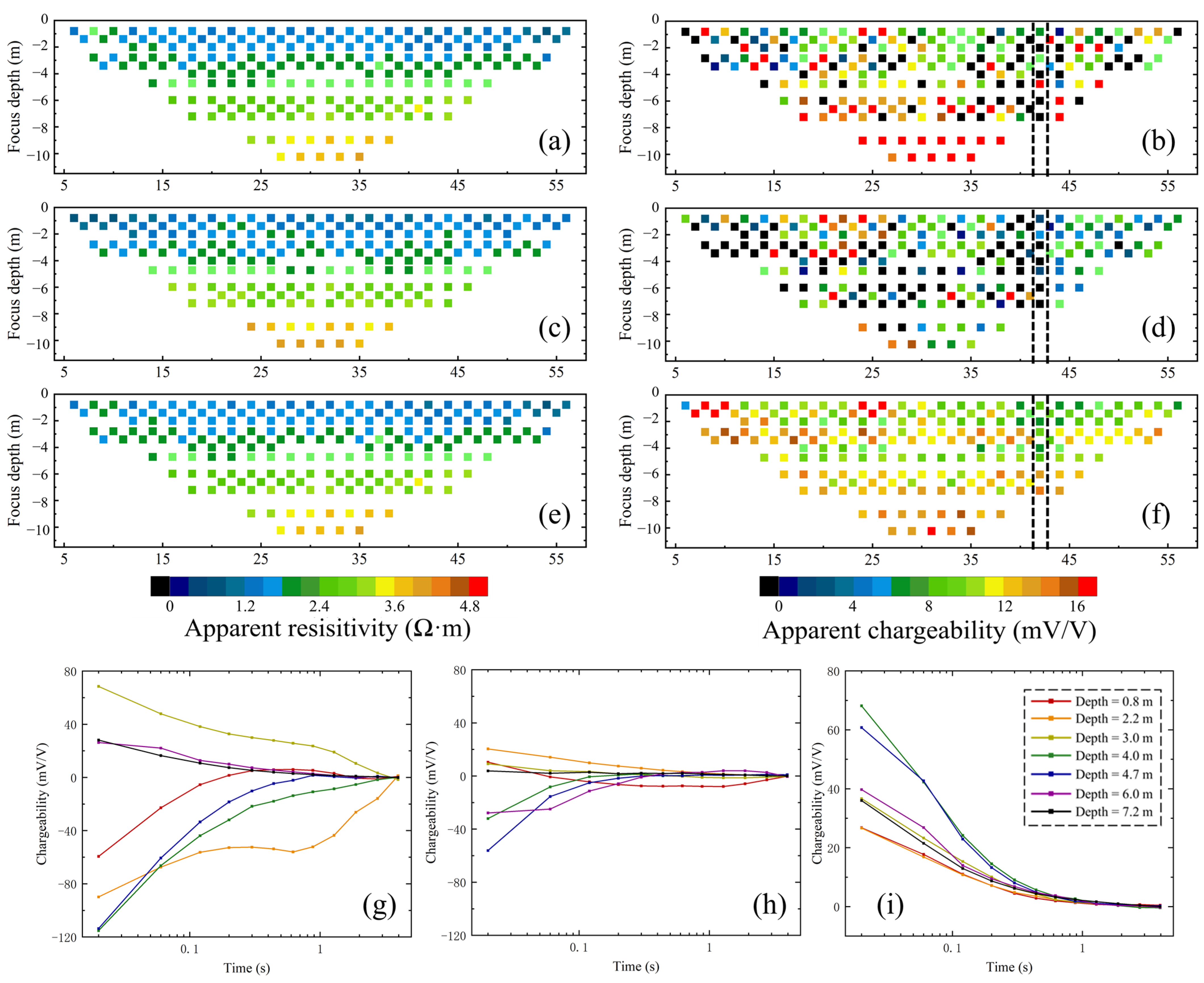
3.1. Data Quality Analysis of Field IP Data

The apparent resistivity profile obtained using the single-cable layout (Figure 3a) appears to be quite layered and smooth, with apparent resistivity ranging from around 1 to 4.5 Ω·m. However, the chargeability pseudosection (Figure 3b) shows a severely disturbed appearance and contains a large number of negative values at both small and large focus depths. The resistivity pseudosection measured using double-cable layouts with stainless steel current and potential electrodes (Figure 3c) is very similar to that from the single-cable layout, but the chargeability pseudosection (Figure 3d) also has a severely disturbed and negative appearance. The resistivity pseudosection (Figure 3e) measured using the last method is similar to the one from the single-cable layout, whereas the chargeability pseudosection (Figure 3f) is not repeatable compared to the results of the first two methods. The result shows a smooth and consistent appearance without negative chargeability values.

Figure 3g–i show chargeability decay curves at seven pseudo-depths. The decay curves of three different methods from the same location vary significantly. Most curves exhibit a non-decaying or even an increasing trend with the first two methods. However, all curves show a smooth decay with non-polarized electrodes, and the appearance is not indicated to be influenced by noise.

All of the apparent resistivity data were retained, and the available apparent chargeability data quantity is shown in Table 1. The first two methods left only 48% and 45.4% of the total data. The last method had an effective data utilization rate of 89.5%, and the available data from gate 4 to gate 8 are up to 293 of the total 294 data points. The data of early and late time gates were mostly removed because capacitive coupling is generally serious at early stages after a variation in the current, and the IP signals are low at very late stages, causing the signal to be easily drowned in noise. Both the chargeability pseudosections and decay curves show that the data quality using double-cable layouts with stainless steel current electrodes and non-polarized potential electrodes is visibly better than that using the two other data acquisition methods. The critical factor in obtaining reliable raw data at the site is the application of non-polarization electrodes that can reduce the electrode polarization between the soil and electrode. Thus, only this data acquisition method can obtain credible data at such a low groundwater salinity waste disposal site.

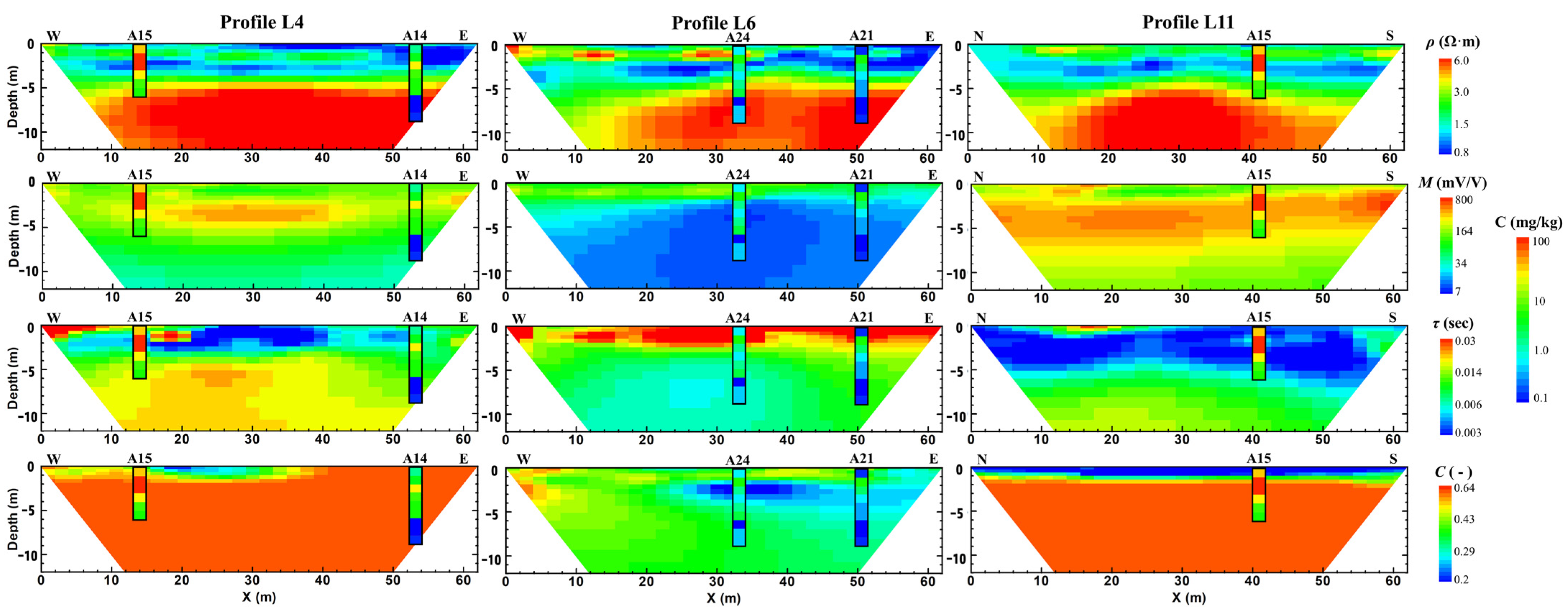
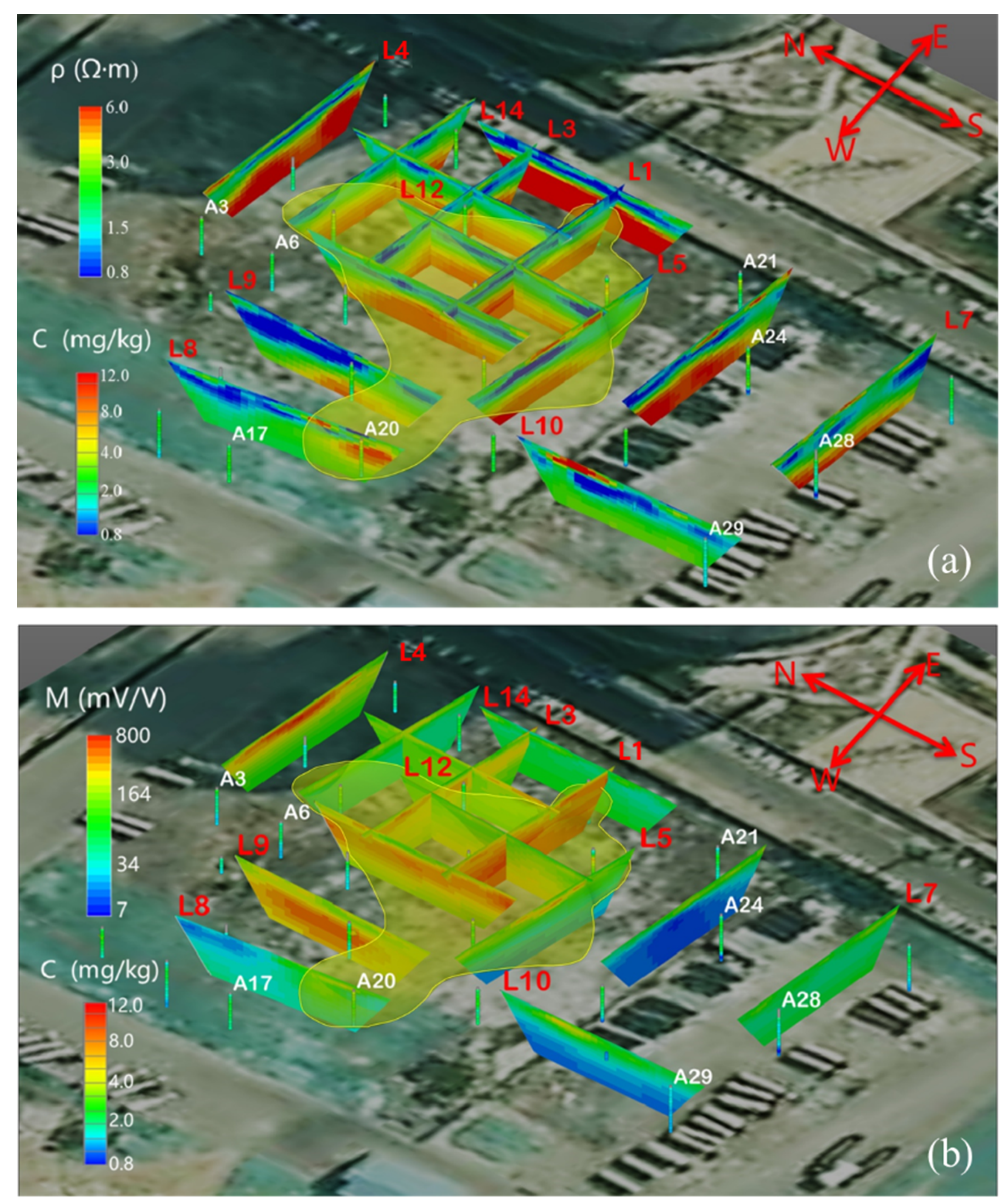
3.2. Inversion Results of Field IP Investigation

In Figure 4, we show the IP inversion profiles for data acquired along L1, L6 and L11 as examples. The profile results are exhibited in terms of the resistivity, chargeability, relaxation time and Cole–Cole exponent. The benzene concentrations from boreholes A14, A15, A21 and A24 were superposed for the interpretation of the TDIP results. The hydrogeological profiles show that the underground medium can be divided into two layers: an upper solid waste layer and the underlying native soil layer up to the depth of investigation. The groundwater geochemical results show that the ion concentration in the solid waste layer is high, and the release of ions at the interface between the pore water and waste could result in increasing conductivity in groundwater and decreasing bulk resistivity. In addition, the moisture content of waste was 59.27%, while those of silty clay and silt were 26.34 and 21.55 percent, which also caused the decrease in resistivity. Therefore, the top solid water layer would show a low-resistivity response, and the underlying native soil would indicate a relatively high-resistivity response, which agrees with the resistivity imaging profiles along all profiles.

Previous borehole surveys show that solid waste is made up of several different types. However, the distribution of waste types cannot be delineated because of the discontinuous underground information between sparse boreholes. Meanwhile, the chargeability profiles can be classified into two distinct types: dramatically high chargeability (e.g., L1 and L11) and normal chargeability (e.g., L6). The IP response in the high-chargeability profiles is much higher than those observed from unconsolidated soils. Such a high polarization magnitude is common in the presence of metal substances. Almost the whole profile of L11 exhibits high chargeability, including the native sediments below 5 m. We assume that the solid waste in high-chargeability areas contains metallic content and the weak IP response of native soil was shielded by the high-IP response from metal substances.

Similarly, the profiles of the relaxation time and Cole–Cole exponent can also be classified into two distinct types based on different characteristics. The high-chargeability profiles L1 and L11 show a short-relaxation-time response, which is also interpreted as the existence of metals. The relaxation time for metallic polarization is rapid because the mobility of the n- and p-charge carriers is much higher than the mobility of the ions in the pore water [49]. The Cole–Cole exponent describes the broadness of the relaxation time distribution and is usually high in a porous medium with metallic particles [50,51]. Therefore, the Cole–Cole exponent is high in profiles L1 and L11, while it is low in profile L6.

It is worth noting that the IP parameters will indicate an anomalous response when organic contaminants are present. However, the IP parameters did not vary significantly in the zones of high and low benzene concentrations. We assume that the underground medium with dramatically low resistivity and high chargeability dominated the direct current and IP effect. Thus, it is insensitive to organic contamination.

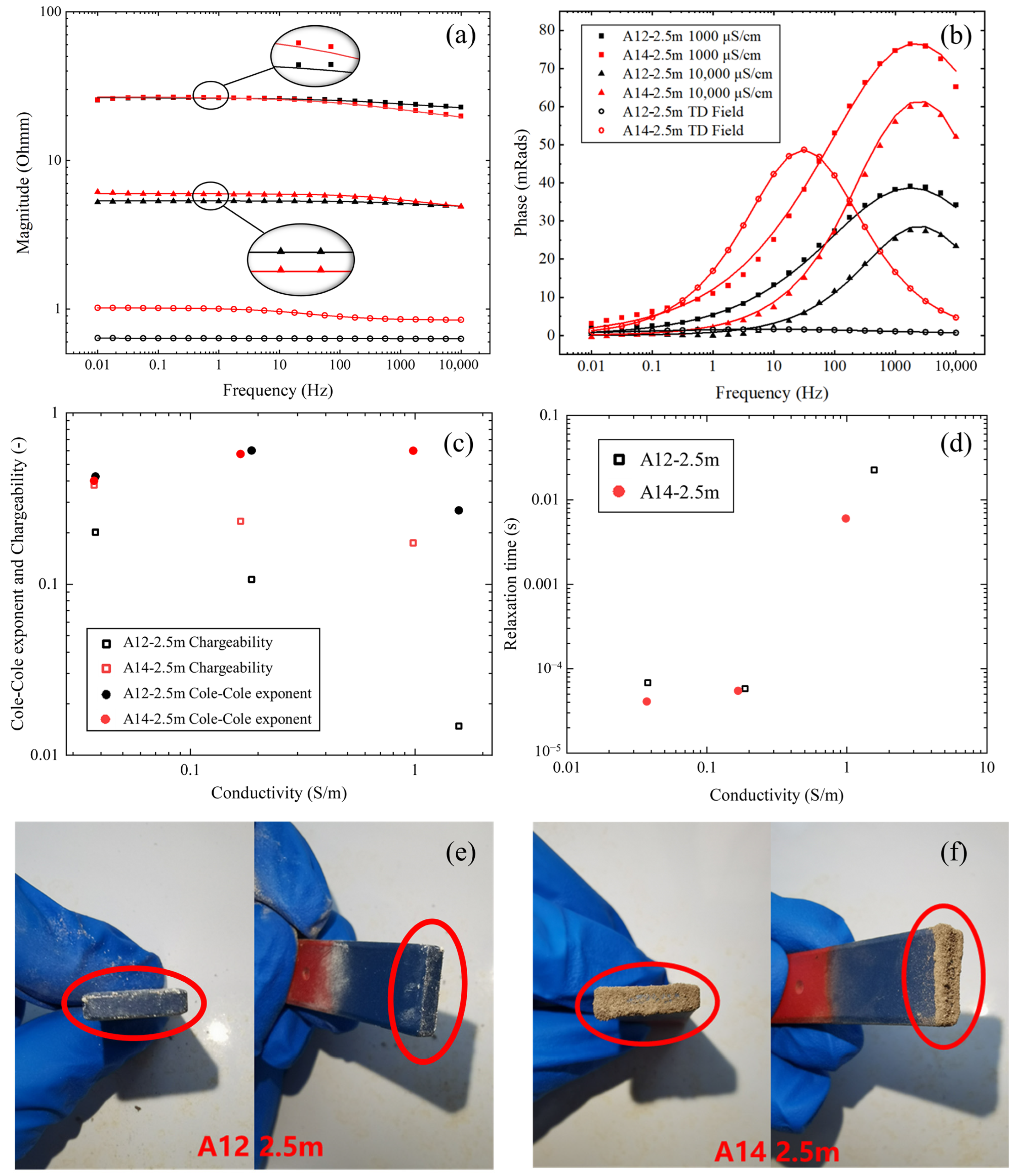
3.3. FDIP Experiment Results

The spectral information of the FDIP experiment on samples and the comparison with field results are shown in Figure 5. The complex resistivity magnitudes measured in the laboratory were dominated by the conductivity of the pore water, with 26 Ω·m for a pore water conductivity of 1000 μS/cm and about 6 Ω·m for 10,000 μS/cm. The slight difference in FDIP complex resistivity magnitudes for the same pore water conductivity from three samples may be caused by differences in porosity or surface conductivity. The large differences in TDIP resistivity magnitudes between two samples could be interpreted as differences in groundwater conductivity. The magnitudes in A12-2.5m and A14-2.5m are lower than the FDIP results with a pore water conductivity of 10,000 μS/cm, which is interpreted as the groundwater conductivity in the solid waste layer being higher than 10,000 μS/cm, as proved by the borehole results (22,490 μS/cm for 3 m and 25,130 μS/cm for 3.5 m).

The measured phases and magnitudes of all laboratory samples were fitted using the Cole–Cole model, and the four parameters of resistivity, chargeability, relaxation time and the Cole–Cole exponent were acquired. The solid lines in Figure 5 show that the fitted curves and the fitting degrees of the Cole–Cole model are high. The measured phases of all laboratory samples have obvious peaks at high frequency, which describe a similar particle size distribution in three samples, and this is proved by the inverted relaxation time (Figure 5d) because the relaxation time is relevant to the grain radius [52]. The inverted chargeability (Figure 5c) shows that A14-2.5m is higher than A12-2.5m in each conductivity, and the chargeability of both samples is higher than 100 mV/V, which is interpreted as a finer particle size. However, the chargeability of A12-2.5m from the field survey is quite low (only 14.79 mV/V). One such large difference between the laboratory and the field is attributed to the scale effect [44]. In addition, the chargeability is dependent on the conductivity since lower conductivity commonly leads to a greater impact on the current transferring through the electrical double layers around the grains [53]. Therefore, larger chargeability values were collected from samples from a lower-conductivity environment. The Cole–Cole exponent is similar in two samples, but the field results show a large difference. The Cole–Cole exponent in A14-2.5m is relatively high, and the high Cole–Cole exponent is suspected to be due to the presence of metal substances [54]. In general, the relaxation time constant is lower in laboratory measurements (<10⁻⁴ s) and smaller than the field data (10⁻² s). The short relaxation time indicates the existence of fine materials.

The XRF results (

Table 2. XRF values of the soil samples, in mg/kg.

Borehole and Depth	Cr	K	Ca	Sc	Mn	Fe	Cu	Zn
A12-2.5m	123.59	2506	215,621	1588	280	9576	58	152
A14-2.5m	139.56	4135	106,089	811	449	31,683	56	150

) indicate that the A14-2.5m samples contained more Fe (31,683 mg/kg) compared to A12-2.5m (9576 mg/kg). This confirms the presence of polarizable minerals in A14-2.5m. In addition, the magnet attracted a large number of particles when it touched the A14-2.5m sample, while few particles were attracted when it touched A12-2.5m (Figure 5c,d), which further proved the presence of metal substances in the sample of A14-2.5m. The higher metallic content is consistent with the high chargeability of A14-2.5m.

3.4. Contaminant Concentration from Sampling

The main contaminant was benzene, according to the geochemical analysis results of 189 soil samples for 64 organic contamination indexes. The benzene concentration results from all samples are shown in

Table 3. Benzene concentration results for soil samples collected from the boreholes, in mg/kg.

Borehole	0.5 m	1.5 m	2.5 m	3.5 m	4.5 m	5.5 m	6.5 m	8 m
A1	0.07	1.28	0.50	0.39 *	0.11	—
A2	—	0.10	0.3 *	0.33	0.12	—
A3	3.12	0.37	0.43 *	0.28	0.07	0.08	—	—
A4	1.60	1.90	2.853 *	1.08	0.22	0.30
A5	23.90	19.60	15.75 *	0.71	0.13	—	—	—
A6	0.43	0.89	0.99 *	0.15	0.05	0.05	—	—
A7	0.46	0.31	0.08 *	—	—	—	—	—
A9	1.35	5.10	2.12 *	0.79	0.17	—	—	—
A10	2.41	1.95	1.23 *	0.09	0.14	—
A11	—	2.37	0.37 *	0.17	0.11	0.10
A12	0.00	0.19	1.88 *	0.39	0.17	0.06	0.05	0.03
A13	0.12	1.77	1.70	0.59 *	0.26	0.18	0.03	0.04
A14	1.51	2.33 *	15.90	7.84	2.91	3.06	0.05	0.00
A15	24.80	2460.00	183.00 *	12.50	7.21	3.46
A16	0.55	5.30	3.65 *	0.33	0.16	0.07
A17	0.34	1.78	1.74	1.38 *	0.52	0.44
A18	0.26	292.00	48.30 *	7.15	1.77	1.33	—	—
A19	45.50	6.99	16.80	4.11 *	2.57	1.20
A20	38.70	15.60	4.21	3.60 *	0.54	0.06
A21	0.12	3.30	1.51 *	0.29	0.18	0.18	0.00	0.00
A23	1.06	3.32	3.63 *	0.34	0.99	0.76	—	—
A24	0.51	3.20	1.30 *	0.57	1.10	1.72	0.01	0.26
A25	2.77	1.07	1.25 *	0.43	0.28	0.01	—	—
A26	0.03
A27	0.35	0.89 *	1.78	0.52	0.30	0.11	0.04	0.01
A28	—	0.70	0.12	0.09	0.37	0.08	0.00	0.85
A29	0.11	0.08	0.1 *	0.04	0.06	0.04	0.05	0.02

* The average of two repeated samples. — The concentration was below the detection limit (1.9 μg/kg).

. The highest concentration of 2460 mg/kg was found in borehole A15 at a depth of 1.5 m. Benzene levels above 4 mg/kg were found in eight boreholes (A5, A9, A14, A15, A16, A18, A19 and A20), and this level is the threshold value for soil remediation adopted from the Soil Environmental Quality Risk Control Standard for Soil Contamination of Development Land (Ministry of Ecology and Environment of the People’s Republic of China, GB 36600-2018).

In general, contaminants were basically distributed in the center of the survey area, with lower distributions in the south and north. The vertical distribution first increased and subsequently decreased, mainly in the range from 0.5 to 4.5 m below the ground surface. Most of the contaminated samples came from the solid waste layer, and the original sediment layer was less contaminated due to the low-permeability silty clay and silt beneath the wastes.

4. Discussion

4.1. Verification with Laboratory Soil Samples and IP Field Survey

According to the laboratory FDIP sample analysis results, the calculated Cole–Cole spectral curves from field TDIP data were not in good agreement with laboratory measurement results (Figure 5b). One reason is that the porosity of samples would vary when they were transferred from the field to the laboratory column. Large variations between field and soil core samples can be anticipated to result in more differences in the size and location of relaxation peaks [52]. Scale effects are also a possible factor for the differences between the results of the field and laboratory [55]. The measurement scale in the field is roughly d³ (where d is the electrode spacing; in this study, it is 2 m), but the measurement scale in laboratory tests is about 10 cm³. A large sample volume may contain some fractures and preferential flow paths that may change the resistivity in the field. In addition, Cole–Cole models utilized for TDIP inversion just fit a single relaxation peak and do not consider the spectral information at other frequencies. The frequency range of the laboratory FDIP measurements is 0.01–10,000 Hz in this research, while the waveform period for the TDIP survey is 4 s, and the sampling frequency is 1000 Hz, corresponding to 0.25–500 Hz in the frequency domain according to the Nyqvist sampling theorem [56], whereas the true frequency range is reduced by the gating of full-waveform IP data and the removal of early-time data. Although full-wave inversion was used, the first gate starts at 20 ms, which means that frequencies above 50 Hz are absent in the TDIP data information. Thus, the spectral curves from TD data at high frequencies/short times are not dependent on the FD results [44].

The correlation between conductivity from laboratory measurements and conductivity from the field TDIP survey is shown in Figure 6. The selection of soil samples in the survey area for comparison and analysis was based on the following three criteria: (1) Boreholes only within a horizontal distance of 2 m (one electrode spacing) from TDIP survey lines were chosen. (2) The depth of soil samples was only within the depth of investigation of TDIP profiles. (3) The interpolated values of model cells according to the actual position and depth of borehole samples were selected. Based on the above criteria, a total of 78 soil samples in 11 boreholes out of 196 soil samples in 29 boreholes were qualified for the correction plot.

In addition, the range of conductivities measured in the laboratory is large (about 0.4 to 20 mS/cm), while the range of field results is limited (1 to 17 mS/cm). The conductivity measured in the laboratory decreases quickly with depth, while that measured in the site decreases slowly with depth. One reason is that the inversion strategy follows a smooth constraint, resulting in the maximum conductivity being less than the true value and the minimum conductivity being greater than the true value [57]. Moreover, the inverted parameters are influenced by model constraints and a resolution that decreases with depth [58]. When the low-resistivity layer overlies the high-resistivity layer, the interface of inversion results between them is gradual, and the depth of the interface may be overestimated. Generally, the inverted resistivity value is smaller than the true value of resistivity for the underlying high-resistivity layer, causing the conductivity measured in the field to be higher at a large depth, which will be further proved in Section 4.4.

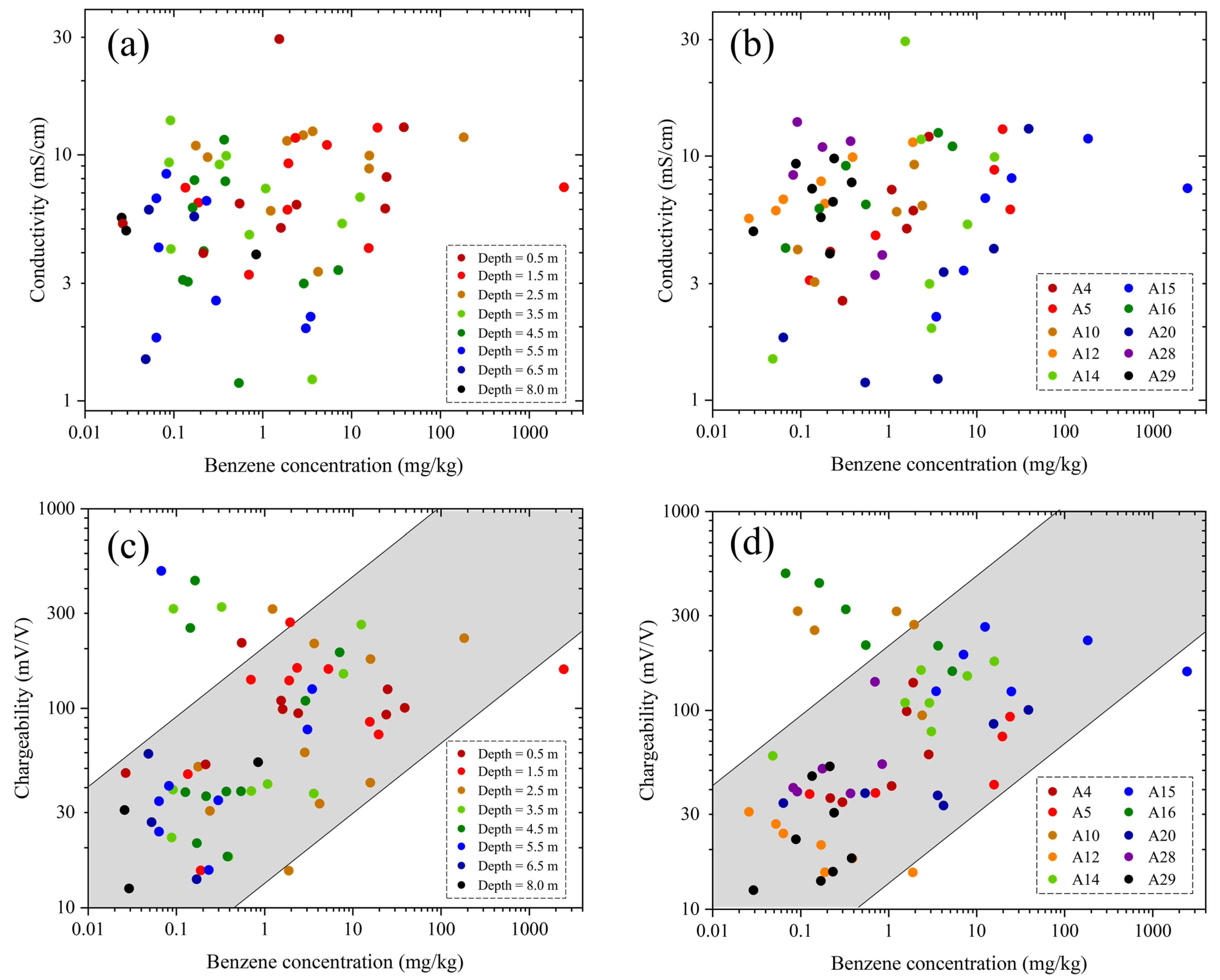
4.2. TDIP Parameters versus Benzene Concentration

The organic contamination has strong responses in relation to conductivity and chargeability [24,25,26], so those parameters were chosen to analyze the correlation with benzene concentration. The correlation plots are shown in Figure 7. As we all know, benzene is a light non-aqueous phase liquid (LNAPL), which is a type of non-conductive organic contaminant. When the conductive groundwater in pores is replaced by non-conductive benzene, the conductivity measured in the field will decrease. Thus, the conductivity will decrease with increasing benzene concentration [59]. However, no correlation could be established between the conductivity and benzene concentration for the current dataset (Figure 7a,b). According to Figure 7a, the benzene concentration decreases with increasing depth, while the conductivity does not increase with depth. The increase in ion concentration in the pore water seems to cause the conductivity to increase vertically, which outbalances the increase in benzene concentration.

Horizontally, the boreholes with a high benzene concentration mainly include A5, A14, A15 and A20 (Figure 7b). The conductivity of those samples did not show an obvious decrease compared to the low-concentration samples. We speculate that the conductive underground medium in the solid waste layer is hardly affected by the resistive benzene contaminant considering the relatively low concentration (<300 mg/kg, except for A15-1.5m). Therefore, it is difficult to distinguish between low-concentration organic contamination and non-contamination at sites with low background resistivity.

Theoretically, the replacement of pore water by organic contaminants will repress the Stern layer and membrane polarization, resulting in decreasing chargeability. For less organic-contaminated sites, the organic contaminant is present as isolated blobs in the pores of the underground media. The oil–water interfaces will form an electrical double layer (EDL) like the EDL of the grain–water interface, resulting in increasing chargeability [25]. However, the chargeability in this site is dramatically high due to the presence of metallic substances. The secondary voltage decays with the drift of the charge carriers in the metallic grains, and hence, ion migration in the EDL is neglected because of their low concentrations [49]. As a result, we speculate that a correlation also could not be established between the chargeability and benzene concentration. However, a slightly positive correlation can be noticed in the gray zone (Figure 7c,d). Most samples are within the gray area, except for the ones in boreholes A10 and A16. Such large variations in chargeability are clearly not caused by differences in benzene contamination concentrations. According to differences in chargeability, solid waste is divided into two different types in the previous section. We assumed that benzene contamination is mainly present in solid waste with high chargeability. This type of solid waste is the source of benzene contamination. Thus, we can indirectly delineate the potential organic contamination by classifying the solid waste types.

4.3. Organic Contamination Constrained with Chargeability

The spatial distribution of the benzene concentration and the TDIP survey results in the study area are shown in Figure 8. The benzene concentration is shown in the interpolated image with semi-opaque volumes indicating a concentration over 4 mg/kg, and the resistivity and chargeability are shown in the fence diagram. Benzene contamination is mainly distributed in the solid waste layer at the center and extends to the east and west boundaries at boreholes A14 and A20, respectively. The northern and southern boundaries are around profiles L2 and L5, respectively. No resistivity anomalies were found in the contaminated area.

A low spatial correlation between contamination distribution and chargeability is found in Figure 8b. The contaminant is mainly distributed in the center of this area, where the chargeability is high. The high-chargeability response was proved to link to the presence of Fe hereinabove, and another major difference between the two solid waste types is Ca (Table 2). The main solid wastes are salt mud, white mud, coal fly ash and desulfurization gypsum in this site, where the coal fly ash contains a large amount of Fe and the salt mud and desulfurization gypsum contain more Ca. Thus, the solid waste with high chargeability probably consists of coal fly ash, and that with normal chargeability consists of salt mud and desulfurization gypsum. The benzene may have been dumped on the site along with the coal fly ash. However, the boundary of interpolated contaminants does not precisely follow the chargeability result. The contaminant is not found in profile L4 or to the north of L9, where the chargeability is high. The reason is that the correlation between contamination and chargeability is indirect, and the benzene-contaminated areas do not exactly coincide with areas of high chargeability. Even so, the TDIP survey results can help build detailed geochemical investigation strategies: a high borehole density in a high-chargeability zone and a low borehole density in a normal-chargeability zone.

This study provides a new method for contamination characterization at waste disposal sites. Solid waste types can be easily distinguished by geophysical parameters and used to identify contamination sources when the relationship between contaminants and geophysical parameters cannot be established because of the low contamination concentration or complex geophysical background. We therefore summarize the procedure for the integration of geophysical and geochemical methods to delineate a contaminated area at a waste disposal site.

Step 1: Preliminary geophysical investigation. The purpose is to obtain the hydrogeological conditions and to classify the types of solid waste. Step 2: Preliminary geochemical investigation. The position and depth of geochemical investigation are determined by geophysical investigation results. This is to verify hydrogeological conditions and solid waste types and to make an initial assessment of the type and extent of contamination. Step 3: Detailed geophysical investigation. The purpose is to delineate geophysical anomalies in areas of interest and to interpret them in detail. Step 4: Detailed geochemical investigation. The position and depth are determined by the initial geochemical investigation and interpretation results of the detailed geophysical survey. This is to verify interpretation results and to establish a correlation between contamination parameters and geophysical parameters. Step 5: Data fusion. Based on the geochemical and geophysical data, a detailed characterization of the site can be obtained.

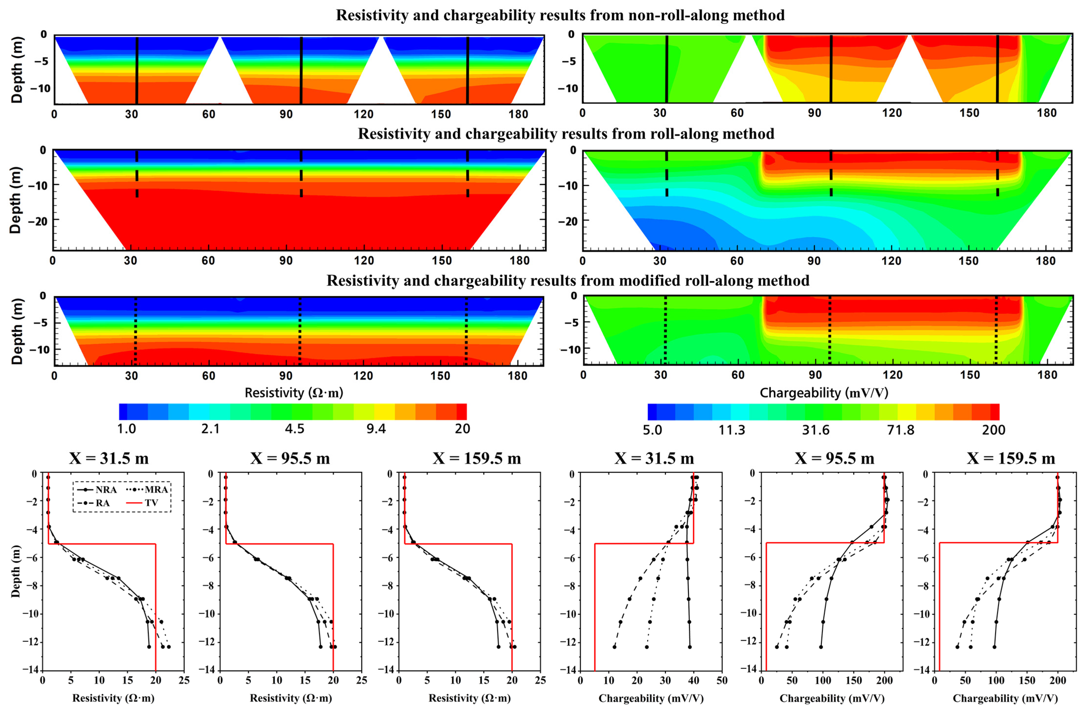
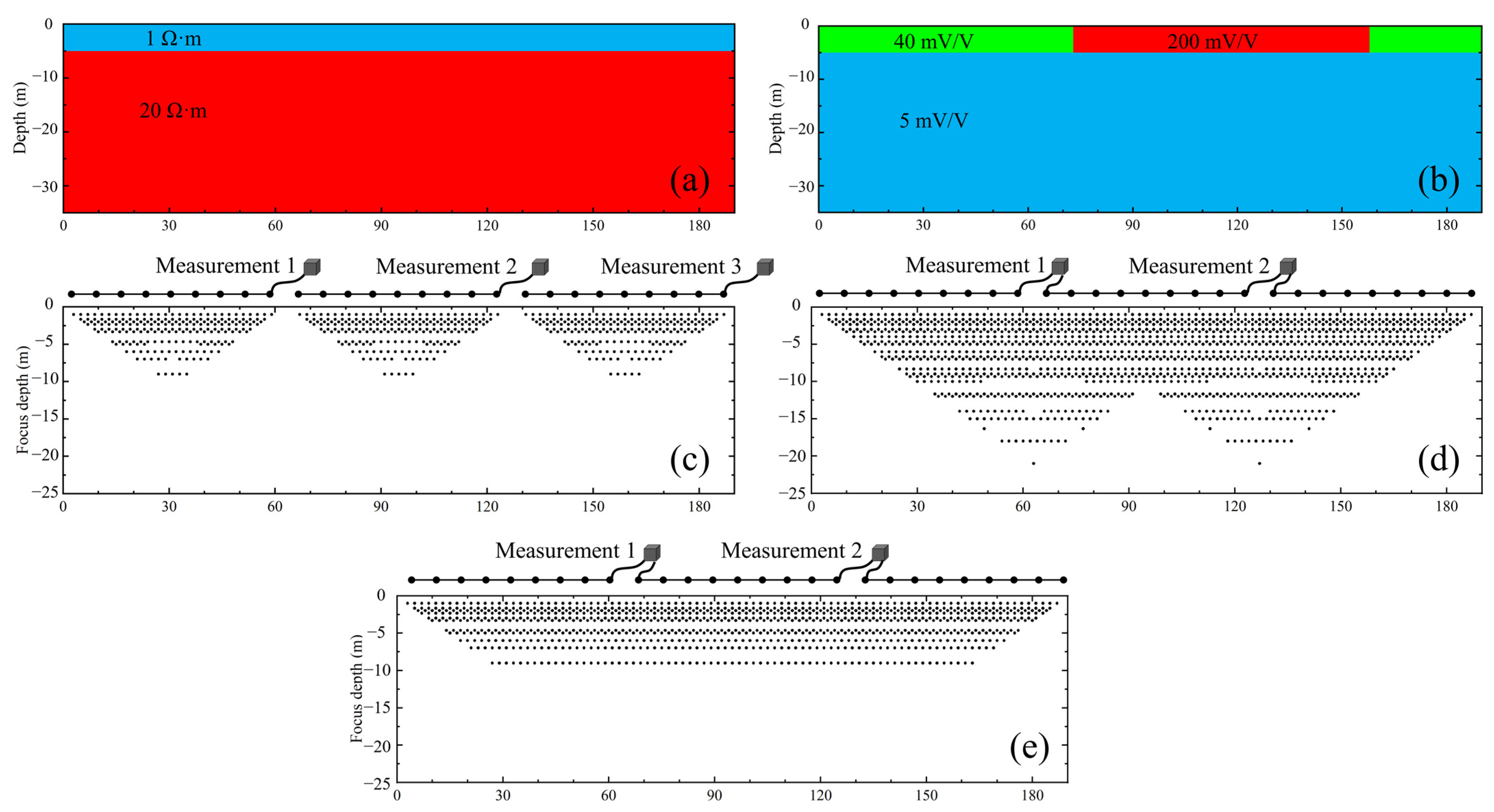
4.4. Improvement of Roll-Along Measurement Protocol

For such a large area of a contaminated shallow groundwater and soil site, fourteen TDIP profiles were measured because of the limited time. However, this is not the best way to integrally delineate the whole waste disposal site, according to Figure 8. A better way is to arrange long profiles across the entire site parallelly, where the distance between profiles is between 10 and 20 m, depending on survey accuracy requirements. For long profiles, the electrode spacing cannot be increased due to resolution issues. Thus, the electrodes and cables should be added in sequence to match the length of the profile. There are two different ways to conduct the long-profile measurement now: the measurement of a single cable in turn (Figure 9c) and roll-along measurement (Figure 9d).

It would be efficient if the profiles were measured separately using the non-roll-along method (NRA). However, conventional electrical protocols have the drawback that the data density is low at both ends of the profile (Figure 9c), resulting in limited contamination or hydrogeological information at both ends. The errors in the splicing of the profiles further devalue the survey results. In contrast, the roll-along method (RA) will acquire data between profiles and improve the reliability there. However, if the contamination at the waste disposal site is mainly distributed at a shallow depth, the DOI of the roll-along method will be much greater than the depth of interest, and the deeper part of the profile will not be effectively used. In addition, the low SNR of raw data and the poor horizontal continuity in deep locations result in limited accuracy, as shown in Figure 9d. Therefore, we modified the roll-along measurement protocol based on the maximum pseudo-depth of the NRA multiple-gradient array. The protocol was modified by adding missing data points between cables. The modified roll-along method (MRA) has higher data density and reliability compared to the NRA method and higher measurement efficiency compared to the RA method. The MRA method takes only 2/3 of the data acquisition time of the RA method because of the reduced data quantity in deep locations.

The feasibility of the three methods was compared using numerical examples based on this waste disposal site. Our resistivity and chargeability models are shown in Figure 9. According to the hydrogeological conditions and solid waste distribution in the current study, a relatively low-resistivity (1 Ω·m) and high-chargeability layer was considered to approximate the solid waste layer (0–5 m). Two different types of solid waste were characterized by high chargeability (200 mV/V) and relatively low chargeability (40 mV/V). The native sediment layer was described by a resistivity value of 20 Ω·m and a chargeability value of 5 mV/V. There were 96 electrodes and 3 cables deployed, and the electrode spacing was 2 m according to the size of this site. The forward simulation was modeled using RES2DMOD, and the data were inverted using RES2DINV (www.geotomosoft.com). There were 882 quadrupole data points collected using the NRA method, and it took approximately 45 min to complete the measurement using data acquisition parameters in this study. The data quantity and acquisition time were 2450 and 125 min for RA and 1638 and 83 min for MRA.

The results are shown in Figure 10. The DOI of the RA method is up to 28 m below the ground surface, while the DOI is about 13 m for NRA and MRA. Qualitatively, the main character of the resistivity profiles is similar for all three methods. In the chargeability profiles, differences are clearly shown, especially in the high-chargeability solid waste area and below. The interface of the chargeability transition is vague, and the chargeability in the native soil layer is overestimated by the NRA method. The chargeability profiles of the other two methods are in better agreement with the numerical model.

In order to quantify the differences in the results obtained by the three methods, the resistivity and chargeability were abstracted from model cells in all depths of 31.5, 95.5 and 159.5 m horizontally. The data below the 13 m depth obtained with RA were removed for direct comparison with the other two methods. Both the resistivity and chargeability results show the estimated values, which are close to the true values (TVs) at shallow depths. However, the values are not in good agreement with TVs in the underlying native sediment layer because of the vertical constraints and a resolution that decreases with depth, especially in the chargeability results. In contrast, the RA method gives results closer to TVs due to high data density, while the results of the NRA method are far away from TVs. Although the MRA method has only 2/3 of the data quantity of the RA method, its results are close to those of the RA method. Therefore, our MRA method can be used to delineate shallow contamination more efficiently and accurately.

5. Conclusions

Our study reveals a method to constrain organic contamination indirectly by classifying solid waste types with the application of TDIP. For measurements collected using three acquisition methods, we demonstrated that the data quality using stainless steel current electrodes and non-polarized potential electrodes is visibly better. Only by using this acquisition method can reliable data be obtained at such a high groundwater salinity waste disposal site. Our results are useful for contaminated site characterization.

Based on the induced polarization survey, solid wastes can be classified into two distinct types: dramatically high chargeability and normal chargeability values. The presence of metals in wastes was assumed to cause a high-chargeability response, which was proved by the laboratory FDIP measurements and XRF analysis. The geochemical results showed that benzene contamination is mainly distributed in the area with high chargeability, and a low correlation between the benzene concentration and chargeability was established. In addition, we established the correlation between conductivity from laboratory sample measurements and that from the field TDIP survey.

We summarized the procedure for the integration of geophysical and geochemical methods to delineate contaminated areas at waste disposal sites according to this research. A new roll-along measurement method was developed to meet the needs of long and shallow contaminated site surveys. The modified roll-along method has higher data density and reliability compared to the non-roll-along method and higher measurement efficiency compared to the roll-along method.

References

1. Ustra, A.T.; Elis, V.R.; Mondelli, G.; Zuquette, L.V.; Giacheti, H.L. Case study: A 3D resistivity and induced polarization imaging from downstream a waste disposal site in Brazil. Environ. Earth Sci. 2012, 66, 763–772. [Google Scholar] [CrossRef] [Green Version]
2. Kjeldsen, P.; Bjerg, P.L.; Rügge, K.; Christensen, T.H.; Pedersen, J.K. Characterization of an old municipal landfill (Grindsted, Denmark) as a groundwater pollution source: Landfill hydrology and leachate migration. Waste Manag. Res. 1998, 16, 14–22. [Google Scholar] [CrossRef]
3. Christensen, T.H.; Kjeldsen, P.; Bjerg, P.L.; Jensen, D.L.; Christensen, J.B.; Baun, A. Review: Biogeochemistry of landfill leachate plumes. Appl. Geochem. 2001, 16, 659–718. [Google Scholar] [CrossRef]
4. Poulsen, T.G.; Moldroup, P.; Sørensen, K.; Hansen, J.A. Linking landfill hydrology and leachate chemical composition at a controlled municipal landfill (Kåstrup, Denmark) using state-space analysis. Waste Manag. Res. 2002, 20, 445–456. [Google Scholar] [CrossRef] [PubMed]
5. Wemegah, D.D.; Finadaca, G.; Auken, E.; Menyeh, A.; Danuor, S.K. Spectral time-domain induced polarisation and magnetic surveying—An efficient tool for characterisation of solid waste deposits in developing countries. Near Surf. Geophys. 2017, 15, 75–84. [Google Scholar] [CrossRef] [Green Version]
6. Umar, U.M.; Naibbi, A.I. Analysis and suitability modeling of solid waste disposal sites in Kano metropolis, Nigeria. Geocarto Int. 2021, 36, 1409–1427. [Google Scholar] [CrossRef]
7. Bjerg, P.L.; Tuxen, N.; Reitzel, L.A.; Albrechtsen, H.-J.; Kjeldsen, P. Natural attenuation processes in landfill leachate plumes at three Danish sites. Groundwater 2011, 49, 688–705. [Google Scholar] [CrossRef]
8. Baderna, D.; Caloni, F.; Benfenati, E. Investigating landfill leachate toxicity In Vitro: A review of cell models and endpoints. Environ. Int. 2019, 122, 21–30. [Google Scholar] [CrossRef]
9. Khan, M.S.; Shahid, M. Metal−Organic Frameworks for Environmental Remediation; American Chemical Society: Washington, DC, USA, 2021; pp. 171–191. [Google Scholar] [CrossRef]
10. Kamal, S.; Khalid, M.; Khan, M.S.; Shahid, M. Metal organic frameworks and their composites as effective tools for sensing environmental hazards: An up to date tale of mechanism, current trends and future prospects. Coord. Chem. Rev. 2022, 474, 214859. [Google Scholar] [CrossRef]
11. Khan, M.S.; Khalid, M.; Shahid, M. What triggers dye adsorption by metal organic frameworks? The current perspectives. Mater. Adv. 2020, 1, 1575–1601. [Google Scholar] [CrossRef]
12. Rinne, J.; Pihlatie, M.; Lohila, A.; Thum, T.; Aurela, M.; Tuovinen, J.; Laurila, T.; Vesala, T. Nitrous Oxide Emissions from a Municipal Landfill. Environ. Sci. Technol. 2005, 39, 7790–7793. [Google Scholar] [CrossRef] [PubMed]
13. Milosevic, N.; Thomsen, N.I.; Juhler, R.K.; Albrechtsen, H.-J.; Bjerg, P.L. Identification of discharge zones and quantification of contaminant mass discharges into a local stream from a landfill in a heterogeneous geologic setting. J. Hydrol. 2012, 446–447, 13–23. [Google Scholar] [CrossRef]
14. Wang, K.; Reguyal, F.; Zhuang, T. Risk assessment and investigation of landfill leachate as a source of emerging organic contaminants to the surrounding environment: A case study of the largest landfill in Jinan City, China. Environ. Sci. Pollut. Res. 2020, 28, 18368–18381. [Google Scholar] [CrossRef] [PubMed]
15. Lenhard, R.J.; Parker, J.C. Estimation of free hydrocarbon volume from fluid levels in monitoring wells. Groundwater 1990, 28, 57–67. [Google Scholar] [CrossRef]
16. Chambers, J.E.; Wilkinson, P.B.; Wealthall, G.P.; Loke, M.H.; Dearden, R.; Wilson, R.; Allen, D.; Ogilvy, R.D. Hydrogeophysical imaging of deposit heterogeneity and groundwater chemistry changes during DNAPL source zone bioremediation. J. Contam. Hydrol. 2010, 118, 43–61. [Google Scholar] [CrossRef] [Green Version]
17. Liao, Q.; Deng, Y.; Shi, X.; Sun, Y.; Duan, W.; Wu, J. Delineation of contaminant plume for an inorganic contaminated site using electrical resistivity tomography: Comparison with direct-push technique. Environ. Monit. Assess. 2018, 190, 187. [Google Scholar] [CrossRef]
18. Revil, A.; Karaoulis, M.; Johnson, T.; Kemna, A. Review: Some low-frequency electrical methods for subsurface characterization and monitoring in hydrogeology. Hydrogeol. J. 2012, 20, 617–658. [Google Scholar] [CrossRef]
19. Mao, D.; Lu, L.; Revil, A.; Zuo, Y.; Hinton, J.; Ren, Z.J. Geophysical Monitoring of Hydrocarbon-Contaminated Soils Remediated with a Bioelectrochemical System. Environ. Sci. Technol. 2016, 50, 8205–8213. [Google Scholar] [CrossRef]
20. Meng, J.; Dong, Y.H.; Xia, T.; Ma, X.M.; Gao, C.L.; Mao, D.Q. Detailed LNAPL plume mapping using electrical resistivity tomography inside an industrial building. Acta Geophys. 2022, 70, 1651–1663. [Google Scholar] [CrossRef]
21. Leroux, V.; Dahlin, T. Dense resistivity and induced polarization profiling for a landfill restoration project at Härlöv, Southern Sweden. Waste Manag. Res. 2007, 25, 49–60. [Google Scholar] [CrossRef] [Green Version]
22. Donno, G.D.; Cardarelli, E. Tomographic inversion of time-domain resistivity and chargeability data for the investigation of landfills using a priori information. Waste Manag. 2017, 59, 302–315. [Google Scholar] [CrossRef] [PubMed] [Green Version]
23. Flores-Orozco, A.; Gallistl, J.; Steiner, M.; Brandstätter, C.; Fellner, J. Mapping biogeochemically active zones in landfills with induced polarization imaging: The Heferlbach landfill. Waste Manag. 2020, 107, 121–132. [Google Scholar] [CrossRef] [PubMed]
24. Sogade, J.A.; Scira-Scappuzzon, F.; Vichabian, Y.; Shi, W.; Rodi William Lesmes, D.P.; Morgan, F.D. Induced-polarization detection and mapping of contaminant plumes. Geophysics 2006, 71, B75–B84. [Google Scholar] [CrossRef]
25. Johansson, S.; Fiandaca, G.; Dahlin, T. Influence of non-aqueous phase liquid configuration on induced polarization parameters: Conceptual models applied to a time-domain field case study. J. Appl. Geophys. 2015, 123, 295–309. [Google Scholar] [CrossRef] [Green Version]
26. Sparrenbom, C.J.; Åkesson, S.; Johansson, S.; Hagerberg, D.; Dahlin, T. Investigation of chlorinated solvent pollution with resistivity and induced polarization. Sci. Total Environ. 2017, 575, 767–778. [Google Scholar] [CrossRef]
27. López-González, A.E.; Tejero-Andrade, A.; Hernández-Martínez, J.L.; Prado, B.; Chávez, R.E. Induced Polarization and Resistivity of Second Potential Differences (SPD) with Focused Sources Applied to Environmental Problems. J. Environ. Eng. Geophys. 2019, 24, 49–61. [Google Scholar] [CrossRef]
28. Wemegah, D.D.; Fiandaca, G.; Auken, E.; Menyeh, A.; Danuor, S.K. Spectral time-domain induced polarilation and magnetic for mapping municipal solid waste deposits in Ghana. In Proceedings of the 20th European Meeting of Environmental and Engineering Geophysics, Athens, Greece, 14–18 September 2014. [Google Scholar] [CrossRef]
29. Frid, V.; Sharabi, I.; Frid, M.; Averbakh, A. Leachate detection via statistical analysis of electrical resistivity and induced polarization data at a waste disposal site (Northern Israel). Environ. Earth Sci. 2017, 76, 233. [Google Scholar] [CrossRef]
30. Leroux, V.; Dahlin, T.; Rosqvist, H. Time-domain IP and resistivity sections measured at four landfills with different contents. In Proceedings of the Near Surface 2010—16th EAGE European Meeting of Environmental and Engineering Geophysics, Zurich, Switzerland, 6–8 September 2010; p. 9. [Google Scholar] [CrossRef]
31. Gazoty, A.; Fiandaca, G.; Pedersen, E.; Auken, E.; Christiansen, A.V. Mapping of landfills using time-domain spectral induced polarization data: The Eskelund case study. Near Surf. Geophys. 2012, 10, 575–586. [Google Scholar] [CrossRef] [Green Version]
32. Elis, V.R.; Ustra, A.T.; Hidalgo-Gato, M.C.; Pejon, O.J.; Hiodo, F.Y. Application of induced polarization and resistivity to the environmental investigation of an old waste disposal area. Environ. Earth Sci. 2016, 75, 1338. [Google Scholar] [CrossRef]
33. Gazoty, A.; Fiandaca, G.; Pedersen, E.; Auken, E.; Christiansen, A.V.; Pedersen, J.K. Application of time domain induced polarization to the mapping of lithotypes in a landfill site. Hydrol. Earth Syst. Sci. 2012, 16, 1793–1804. [Google Scholar] [CrossRef] [Green Version]
34. Nielsen, T.I. The effect of electrode contact resistance and capacitive coupling on Complex Resistivity measurements. SEG Tech. Program Expand. Abstr. 2006, 25, 1376–1380. [Google Scholar] [CrossRef]
35. Dahlin, T. Short note on electrode charge-up effects in DC resistivity data acquisition using multi-electrode arrays. Geophys. Prospect. 2000, 48, 181–187. [Google Scholar] [CrossRef]
36. Zarif, F.; Kessouri, P.; Slater, L. Recommendations for Field-Scale Induced Polarization (IP) Data Acquisition and Interpretation. J. Environ. Eng. Geophys. 2017, 22, 395–410. [Google Scholar] [CrossRef]
37. Dahlin, T.; Leroux, V.; Nissen, J. Measuring techniques in induced polarisation imaging. J. Appl. Geophys. 2002, 50, 279–298. [Google Scholar] [CrossRef] [Green Version]
38. Dahlin, T.; Leroux, V. Improvement in time-domain induced polarization data quality with multi-electrode systems by separating current and potential cables. Near Surf. Geophys. 2012, 10, 545–565. [Google Scholar] [CrossRef] [Green Version]
39. Gündoğdu, N.Y.; Demirci, İ.; Özyildirim, Ö.; Aktarakçi, H.; Candansayar, H.E. Investigating the Use of Stainless Steel Electrodes with the IP Method: A Metallic Ore Deposit Example. Pure Appl. Geophys. 2022, 179, 265–274. [Google Scholar] [CrossRef]
40. Olsson, P.I.; Fiandaca, G.; Larsen, J.J.; Dahlin, T.; Auken, E. Doubling the spectrum of time-domain induced polarization by harmonic de-noising, drift correction, spike removal, tapered gating and data uncertainty estimation. Geophys. J. Int. 2016, 207, 774–784. [Google Scholar] [CrossRef]
41. Barfod, A.S.; Lévy, L.; Larsen, J.J. Automatic Processing of Time Domain Induced Polarisation Data using Supervised Artificial Neural Networks. Geophys. J. Int. 2020, 224, 312–325. [Google Scholar] [CrossRef]
42. Fiandaca, G.; Ramm, J.; Binley, A.; Gazoty, A.; Christiansen, A.; Auken, E. Resolving spectral information from time domain induced polarization data through 2-D inversion. Geophys. J. Int. 2013, 192, 631–646. [Google Scholar] [CrossRef]
43. Maurya, P.K.; Fiandaca, G.; Christiansen, A.V.; Auken, E. Field-scale comparison of frequency- and time-domain spectral induced polarization. Geophys. J. Int. 2018, 214, 1441–1465. [Google Scholar] [CrossRef] [Green Version]
44. Johansson, S.; Lindskog, A.; Fiandaca, G.; Dahlin, T. Spectral Induced Polarization of limestones: Time domain field data, frequency domain laboratory data and physicochemical rock properties. Geophys. J. Int. 2020, 220, 928–950. [Google Scholar] [CrossRef]
45. Auken, E.; Viezzoli, A.; Christensen, A. A single software for processing, inversion, and presentation of AEM data of different systems: The Aarhus Workbench. ASEG Ext. Abstr. 2009, 2009, 1. [Google Scholar] [CrossRef]
46. Wang, C.; Slater, L.D. Extending Accurate Spectral Induced Polarization Measurements into the kHz Range: Modeling and Removal of Errors from Interactions between the Parasitic Capacitive Coupling and the Sample Holder. Geophys. J. Int. 2019, 218, 895–912. [Google Scholar] [CrossRef]
47. Cole, K.S.; Cole, R.H. Dispersion and absorption in dielectrics I. Alternating current characteristics. J. Chem. Phys. 1941, 9, 341–351. [Google Scholar] [CrossRef] [Green Version]
48. Pelton, W.H.; Ward, S.H.; Hallof, P.G.; Sill, W.R.; Nelson, P.H. Mineral Discrimination and Removal of Inductive Coupling with Multifrequency IP. Geophysics 1978, 43, 588–609. [Google Scholar] [CrossRef]
49. Revil, A.; Florsch, N.; Mao, D. Induced polarization response of porous media with metallic particles—Part 1: A theory for disseminated semiconductors. Geophysics 2015, 80, D525–D538. [Google Scholar] [CrossRef]
50. Mao, D.; Revil, A.; Hinton, J. Induced polarization response of porous media with metallic particles—Part 4: Detection of metallic and nonmetallic targets in time-domain induced polarization tomography. Geophysics 2016, 81, D359–D375. [Google Scholar] [CrossRef]
51. Revil, A.; Sleevi, M.F.; Mao, D. Induced polarization response of porous media with metallic particles—Part 5: Influence of the background polarization. Geophysics 2017, 82, E77–E96. [Google Scholar] [CrossRef]
52. Tarasov, A.; Titov, K. On the use of the Cole–Cole equations in spectral induced polarization. Geophys. J. Int. 2013, 195, 352–356. [Google Scholar] [CrossRef]
53. Slater, L.; Lesmes, D.P. Electrical-hydraulic relationships observed for unconsolidated sediments. Water Resour. Res. 2002, 38, 1213. [Google Scholar] [CrossRef]
54. Revil, A.; Coperey, A.; Mao, D.; Abdulsamad, F.; Ghorbani, A.; Rossi, M.; Gasquet, D. Induced polarization response of porous media with metallic particles—Part 8. Influence of temperature and salinity. Geophysics 2018, 83, E435–E456. [Google Scholar] [CrossRef]
55. Maineult, A.; Revil, A.; Camerlynck, C.; Florsch, N.; Titov, K. Upscaling of spectral induced polarization response using random tube networks. Geophys. J. Int. 2017, 209, 948–960. [Google Scholar] [CrossRef] [Green Version]
56. Johansson, S.; Hedblom, P.; Dahlin, T. Spectral analysis of time domain induced polarization waveforms. J. Appl. Geophys. 2020, 177, 104077. [Google Scholar] [CrossRef]
57. Auken, E.; Christiansen, A.V. Layered and laterally constrained 2D inversion of resistivity data. Geophysics 2004, 69, 752–761. [Google Scholar] [CrossRef]
58. Loke, M.H.; Barker, R.D. Rapid least-squares inversion of apparent resistivity pseudosections by a quasi-Newton method. Geophys. Prospect. 1996, 44, 131–152. [Google Scholar] [CrossRef]
59. Xia, T.; Dong, Y.; Mao, D.; Meng, J. Delineation of LNAPL contaminant plumes at a former perfumery plant using electrical resistivity tomography. Hydrogeol. J. 2021, 29, 1189–1201. [Google Scholar] [CrossRef]
Figure 1. Satellite image showing the measurement layout of the waste disposal site in Shandong Province, China. Time-domain induced polarization (TDIP) profiles are marked with red lines. Soil sample boreholes were arranged around the IP profiles. Two hydrogeological profiles (I–I’ and Ⅱ–Ⅱ’) were located in the north and south of the survey area.
Water 14 03630 g001
Figure 2. The two hydrogeological cross-sections of the waste disposal site. The solid waste overlies the low-permeability silty clay layer and silt layer.
Water 14 03630 g002
Figure 3. TDIP data of profile L1. (a,b) Resistivity and chargeability pseudosections from single-cable acquisition method. (cf) Resistivity and chargeability pseudosections by separating current and potential cables. (c,d) Stainless steel current and potential electrodes. (e,f) Stainless steel current electrodes and non-polarized potential electrodes. (gi) IP decay curves from the pseudosection areas highlighted by the black dotted bordered rectangle in Figure 3b,d,f. Both the chargeability pseudosections and decay curves show that the data quality using non-polarized potential electrodes is better than that using the other two acquisition methods.
Water 14 03630 g003
Figure 4. TDIP inversion results of profiles L1, L6 and L11 superposed with benzene concentration data. The imaging results are expressed in terms of the resistivity, chargeability, relaxation time and Cole–Cole exponent. Inversion results for data collected along all profiles revealed a similar resistivity distribution. The chargeability, relaxation time and Cole–Cole exponent can be classified into two distinct types.
Water 14 03630 g004
Figure 5. Complex resistivity spectra. The spectral information is shown as (a) magnitude and (b) phase measured with FDIP method and calculated with TDIP surveys. The red and black lines in Figure 5 show the fitted curves. The inverted parameters are shown as (c) Cole–Cole exponent and chargeability and (d) relaxation time. Magnet attraction tests were conducted with samples (e) A12-2.5m and (f) A14-2.5m. The magnet attraction test shows the presence of metals in A14-2.5m.
Water 14 03630 g005
Figure 6. Conductivity from field TDIP survey versus conductivity from laboratory measurement. Both the laboratory and field data show that the conductivity was high at shallow depths and low at large depths. The correlation coefficient between conductivity in the field and laboratory is only 0.53. The range of conductivities measured in the laboratory is large (about 0.4 to 20 mS/cm), while the range of field results is limited (1 to 17 mS/cm). Both the laboratory and field data show that the conductivity was high at shallow depths and low in large-depth areas, corresponding to solid waste and native sediments, respectively. However, the correlation coefficient between the conductivity in the field and laboratory is only 0.53. The small correlation coefficient is partly due to the different measurement methods. The measurement method of the field TDIP survey obtains the conductivity of the underground medium, including solid, liquid and gas phases. Thus, the conductivity is influenced by variability from the salinity of groundwater, porosity, water content, pore path, surface conductivity, etc., while laboratory measurements are dominated by the ions in core samples and the soil itself.
Water 14 03630 g006
Figure 7. Resistivity and chargeability versus benzene concentration. No correlation could be established between conductivity (a,b) and benzene concentration, while a slightly positive correlation between chargeability (c,d) and benzene concentration can be noticed inside the gray zone.
Water 14 03630 g007
Figure 8. The spatial distribution of TDIP and geochemical results. (a) Resistivity profiles and (b) chargeability profiles with benzene concentration. The benzene concentration is shown in the interpolated image with yellow semi-opaque volumes indicating a concentration over 4 mg/kg. Benzene contamination is mainly distributed in the solid waste layer at the central part and extends to the east and west boundaries at boreholes A14 and A20.
Water 14 03630 g008
Figure 9. Numerical model configuration and measurement sketch. It shows numerical model setup of resistivity (a) and chargeability (b). Sketches of measurement pseudo data points are shown for NRA (c), RA (d) and MRA (e).
Water 14 03630 g009
Figure 10. The inversion results for numerical simulations. The main character of the resistivity profiles is similar for all three methods. In the chargeability profiles, differences are clearly shown, especially in the high-chargeability area. The RA method gives results closer to TVs due to the larger data quantity, while the results of the NRA method are far from TVs.
Water 14 03630 g010