Article

Novel Salinity Modeling Using Deep Learning for the Sacramento–San Joaquin Delta of California

1
Department of Electrical and Computer Engineering, University of California, Davis, CA 95616, USA
2
California Department of Water Resources, 1516 9th Street, Sacramento, CA 95814, USA
3
Department of Computer Science, University of California, Davis, CA 95616, USA
4
Department of Mathematics, University of California, Davis, CA 95616, USA
*
Authors to whom correspondence should be addressed.
Water 2022, 14(22), 3628; https://doi.org/10.3390/w14223628
Submission received: 1 September 2022 / Revised: 26 October 2022 / Accepted: 4 November 2022 / Published: 11 November 2022

Abstract

:
Water resources management in estuarine environments for water supply and environmental protection typically requires estimates of salinity for various flow and operational conditions. This study develops and applies two novel deep learning (DL) models, a residual long short-term memory (Res-LSTM) network, and a residual gated recurrent unit (Res-GRU) model, in estimating the spatial and temporal variations of salinity. Four other machine learning (ML) models, previously developed and reported, consisting of multi-layer perceptron (MLP), residual network (ResNet), LSTM, and GRU are utilized as the baseline models to benchmark the performance of the two novel models. All six models are applied at 23 study locations in the Sacramento–San Joaquin Delta (Delta), the hub of California’s water supply system. Model input features include observed or calculated tidal stage (water level), flow and salinity at model upstream boundaries, salinity control gate operations, crop consumptive use, and pumping for the period of 2001–2019. Meanwhile, field observations of salinity at the study locations during the same period are also utilized for the development of the predictive use of the models. Results indicate that the proposed DL models generally outperform the baseline models in simulating and predicting salinity on both daily and hourly scales at the study locations. The absolute bias is generally less than 5%. The correlation coefficients and Nash–Sutcliffe efficiency values are close to 1. Particularly, Res-LSTM has slightly superior performance over Res-GRU. Moreover, the study investigates the overfitting issues of both the DL and baseline models. The investigation indicates that overfitting is not notable. Finally, the study compares the performance of Res-LSTM against that of an operational process-based salinity model. It is shown Res-LSTM outperforms the process-based model consistently across all study locations. Overall, the study demonstrates the feasibility of DL-based models in supplementing the existing operational models in providing accurate and real-time estimates of salinity to inform water management decision making.

1. Introduction

1.1. Background

This study develops novel machine learning (ML) approaches in salinity modeling in an estuarine environment. The innovations include (a) proposing inventive ML models never explored in the literature before and (b) a novel application of the proposed ML models at a finer hourly time scale in both simulation and prediction.
Salinity management in estuarine environments can impact the region’s water supply and ecology. Estuarine salinity is linked to changes in migration patterns, spawning habitat, fish distribution, and survivability, and affects the water quality of freshwater withdrawals [1,2]. Globally, many examples of estuarine systems sensitive to salinization exist. In Chesapeake Bay, the largest estuary in the United States, salinity impacts the habitat characteristics and influences the distribution, survival, and growth of a variety of species [1,3]. The Mekong Delta in Vietnam is critically important to the country’s economy and is vulnerable to salinity intrusion due to sea level rise and upstream flow regulation [4]. Mulamba et al. [5] studied the sea-level rise impacts on the lower St. Johns River in Florida, where salinity change due to sea-level rise can potentially alter its estuarine ecosystem and threaten groundwater and surface water supplies. The Murray–Darling Basin Authority is engaged in strategic salinity management in Australia’s Murray–Darling River Basin, where salinization affects municipal, industrial, and agricultural water supply, soil salinity, and ecosystem health [6,7]. Salinity management is actively pursued worldwide and is of particular importance for estuarine environments with significant social, economic, and environmental values, including the Sacramento–San Joaquin Delta in California, United States (U.S.).
The Sacramento–San Joaquin Delta (Delta) is the largest estuary on the west coast of the U.S. and is formed by the confluence of the two largest river systems in California, the Sacramento River and the San Joaquin River. The river flows across the Delta and through the Delta’s downstream boundary at Martinez and into San Francisco Bay. Tides from the Pacific Ocean bring salty water upstream into the Delta. The Delta provides a habitat for 750 species of animals and plants and is a globally important biodiversity hot spot [8,9]. The Delta also provides drinking and irrigation water for California through the state, federal, and local water distribution systems, including the State Water Project (SWP) and the Central Valley Project (CVP). The SWP and CVP projects provide water to over 25 million people and 15,000 km2 of farmlands [10]. The Delta is also used by millions for recreation and transportation [11]. Upstream riverine runoff (typically controlled by reservoirs) provides water to meet the water supply needs of the projects, and to meet Delta salinity requirements for both agriculture and wildlife. Within the Delta, consumptive uses of water include evaporation, seepage, and crop evapotranspiration. Salinity levels across the Delta depend upon the complex interactions between fresh water and seawater, which vary by location and are affected by river channel geometry, physical structures such as gates and barriers, diversions, and upstream reservoir releases.

1.2. Literature Review

Optimizing the operation of the SWP and CVP requires estimating salinity for a wide range of climate and operational scenarios. Process-based models have been traditionally developed and utilized for this purpose [12,13,14,15,16,17,18,19,20]. However, applying these models can be time-consuming, particularly in studies that require numerous model runs with long simulation periods. There is a need for fast simulation models with reasonable accuracy. Data-driven ML models have been explored to that end.
The earliest attempt was probably using the multi-layer perceptron (MLP), a type of artificial neural network (ANN), to simulate flow–salinity relationships in the Delta [21]. The study developed MLP models with one hidden layer or two hidden layers and showed that they could outperform empirical models significantly. The MLP model was refined later in terms of (a) identifying the most effective input features and training strategy; (b) increasing their robustness by training them using a variety of hydrology and operational conditions; and (c) simplifying their implementation into operational water planning models [22,23,24,25]. The resulting MLP model with seven input variables and two-hidden layers (with eight and two neurons, respectively) was implemented into California’s latest water resources planning model, CalSim3 [26]. CalSim3 simulates the operations of SWP and CVP under different planning scenarios constrained by regulatory requirements, including allowable salinity levels at various locations across the Delta [26]. Ref. [27] further enhanced the MLP models of [26] in the context of (a) changing the learning paradigm from single-task learning (one MLP per study location) to multitask learning (MTL; one MLP model for all study locations together); and (b) adding a convolution layer before the hidden layers to pre-process input data. These enhancements helped reduce training time and increase the accuracy of the salinity estimates.
In addition to simulating the flow–salinity relationships, ANNs have also been developed to emulate process-based models directly in the Delta. Ref. [2] incorporated the Bayesian ANNs with the delta salinity gradient (DSG) model [17] in a hybrid manner for salinity simulation in the Delta. Ref. [28] utilized ANNs to emulate DSM2 in simulating volumetric fingerprints of flow sources for several study locations across the Delta. Salinity levels at these locations were then derived by multiplying the fingerprints by their corresponding salinity levels at flow source locations. Ref. [10] developed deep learning models, including the long short-term memory (LSTM) networks and convolutional neural networks, to emulate a salinity generation model at the downstream boundary of the Delta. Ref. [29] explored the use of both conventional ML models and deep learning models in emulating DSM2 for salinity estimation at 28 locations across the Delta. However, Ref. [29] did not explore the forecasting capability of the ML models and focused only on the daily scale using simulated salinity data.
Despite their scientific advances and practical values, those Delta salinity ML studies generally have four limitations in common [29]. Firstly, the ML models developed in these studies were mostly applied in simulating salinity under different planning scenarios. The forecasting capability of the ML models was largely unexplored. Reliable and intelligent forecasting is one major practical application for water-resource studies. Over the past decades, machine learning (ML) methods have gained more and more popularity in this area [30,31], due to their ability to handle big data at different scales as well as their flexible structure for identifying non-linear and complex relationships between input and output data. Researchers worldwide have applied novel ML methods in forecasting various variables that are important to water resources management, including streamflow [32,33,34,35,36]; groundwater level [37], groundwater quality [38], groundwater storage change [39], and sediment [40,41], among others. Popular ML algorithms explored include random forest [42,43,44], artificial neural network [45,46], support vector regression [45,47], LSTM [48], regression trees [49], extreme learning machine [45,50], wavelet transform [46,50,51], and adaptive neuro-fuzzy inference system [50,51].
Secondly, those Delta salinity ML studies focused on daily or coarser temporal scales probably due to the prohibitively expensive computing requirement associated with finer time scales. However, sub-daily scales (e.g., tidal scale, hourly scale) are also meaningful for water resources planning and management practices in the Delta. For instance, farmers may need to make water diversion schedules on when to pump water from Delta channels to irrigate their crop lands during a day. Understanding the sub-daily variations of salinity would help inform their relevant decision making to avoid diverting salty water that may have a detrimental effect on crops.
Thirdly, ML models in those studies were typically trained using salinity simulations from process-based models. Simulated data are generally “noise-free”, as they follow the physical laws embedded in the advection–dispersion governing equations hardwired in process-based models. This characteristic makes it straightforward for ML models to learn the underlying patterns or signals in simulated data. This limits the application of those ML models for certain applications, including forecasting. To forecast the spatial and temporal variations of salinity in the near future, it would be ideal for the ML models to be trained and tested using field observations directly so that they can be utilized to predict what would happen in the field. These field observations reflect the real-world salinity conditions containing information not captured by process-based models, which are, at most, simplified representations of reality.

1.3. Scope of the Current Work

The current study attempts to tackle these limitations highlighted above. Specifically, built upon the success of previous studies, particularly the study of [29], which developed four ML models (MLP, LSTM, GRU, and ResNet) to simulate salinity at multiple locations in the Delta, this study proposes two novel ML models, Res-LSTM and Res-GRU, which are less complex but more efficient compared to their vanilla versions (i.e., LSTM and GRU). This study utilizes salinity observations as the target to train these six ML models and assesses their performance on both daily and hourly time scales. Moreover, this study explores the forecasting capability of the two proposed novel ML models. Furthermore, the study discusses the overfitting potential of the proposed models and evaluates model performance against that of a process-based model.
The paper is organized as follows. In Section 2, we describe the methodology applied, including the study ML models proposed and their setup, study locations, study dataset, and study metrics. In Section 3, we illustrate the performance of these models as well as their forecasting capability. In Section 4, we discuss the results, scientific and practical values of the study, and potential future work. The study is concluded in Section 5.

2. Methodology

2.1. Study Area and Dataset

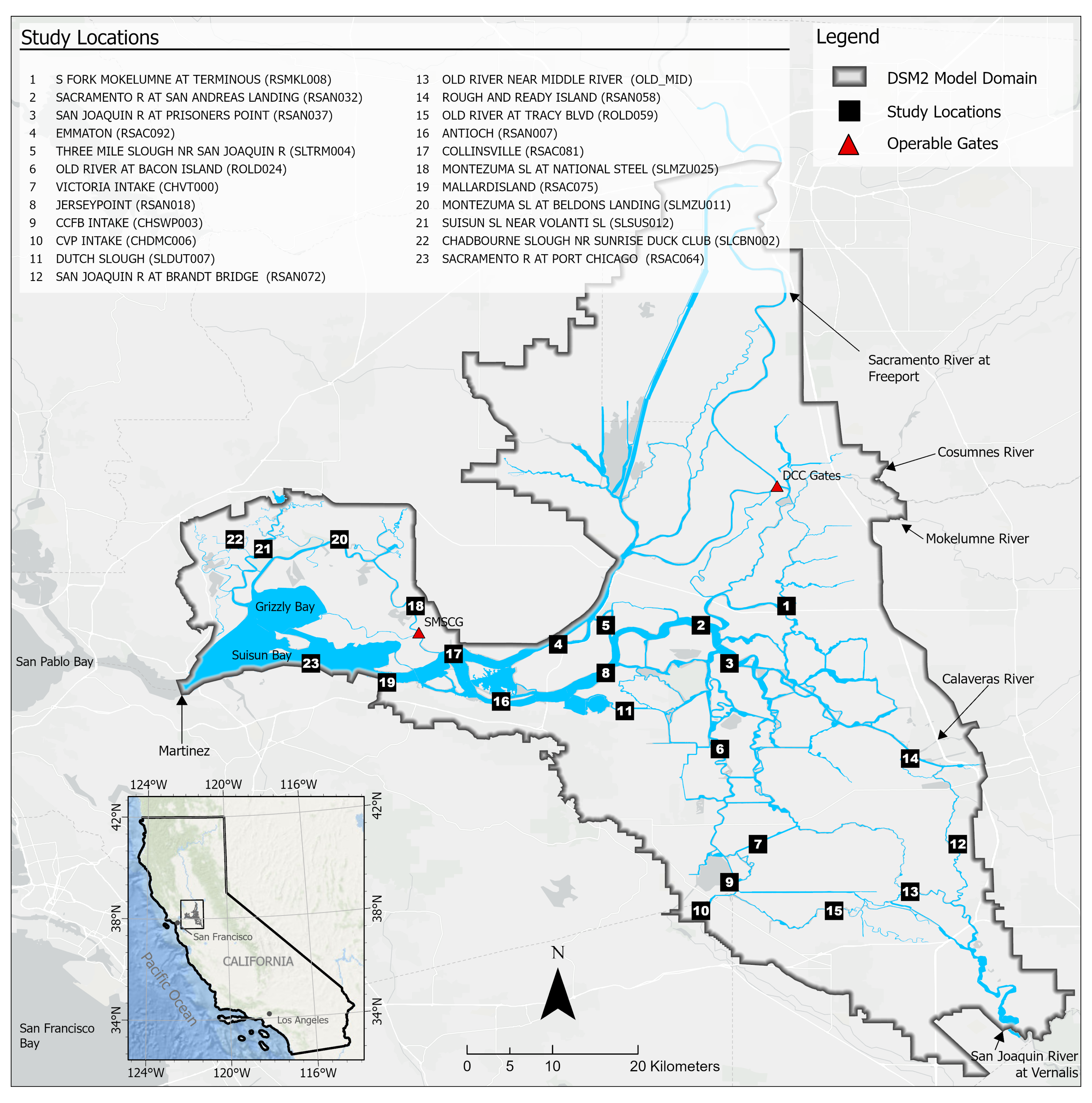
This study exemplifies the development and use of novel ML models in an estuarine system: the Delta of California (Figure 1). The Delta is a transition zone between freshwater and saltwater, where freshwater inflows from the Sacramento and San Joaquin rivers are conveyed westward toward the San Francisco Bay through a series of channels and tributaries. Managing Delta salinity is important to maintain the region’s ecological health, freshwater water supply reliability, and regulatory compliance. Salinity is monitored at sparse locations across the Delta and is typically represented as electrical conductivity (EC) in micro-Siemens/cm ( μ S/cm) which indicates the amount of dissolved salt in water. Specifically, this study focuses on 23 salinity-monitoring locations with a reasonably long record of observed data (Figure 1). These locations include freshwater pumping locations, key flow junctions, and locations of ecological significance in the Delta. Hourly salinity measurements during the study period from 1 January 2000 to 31 December 2019 at these 23 stations are used for ML model training and testing.
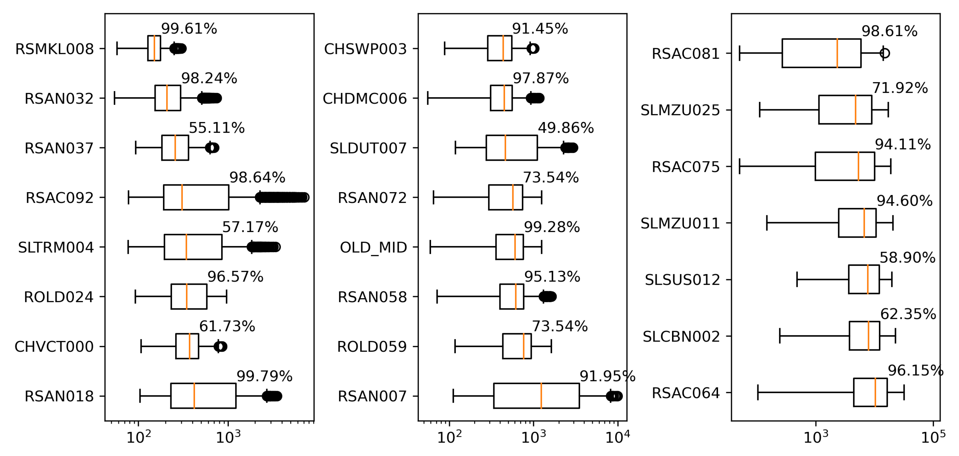
Salinity in the Delta can vary between fully marine to near-zero, depending on the location and interaction between tides and freshwater inflows [52]. Figure 2 visualizes the range of EC values at each station over the 20-year study period. The orange line on each box represents the median values of the corresponding metrics for each of the 23 study locations. Each box represents the interquartile range from the 25th to the 75th percentiles. The location of the upper bar indicates the maximum metric value within 1.5 times the interquartile range above the 75th percentile. The location of the lower bar indicates the minimum metric values within 1.5 times the interquartile range below the 25th percentile. The open circles represent outliers. Figure 2 illustrates that the EC between the least saline and most saline locations can span two orders of magnitude. Generally, water is least saline toward the northern Delta, where lower salinity water from the Sacramento River and eastern tributaries (e.g., Cosumnes River, Mokelumne River, and Calaveras River) enter the Delta. The northernmost locations considered in this study (RSMKL008 #1, RSAN032 #2 and RSAN037 #3) exhibit median EC between 100 and 300 μ S/cm. Median salinity near the major pumping locations (CHVT000 #7, CHSWP003 #8, CHDMC006 #9) ranges from 350 to 450 μ S/cm. San Joaquin River inflows into the southern Delta (RSAN072 #12) have a higher median EC between 600 and 800 μ S/cm, due to having higher salt content from agricultural drainage [53]. In the brackish Suisun Marsh (SLMZU011 #20, SLSUS012 #21, SLCBN002 #22), where the saltwater from the San Francisco Bay meets the freshwater from the Sacramento and San Joaquin Rivers, the median salinity ranges from 8000 to 10,000 μ S/cm. The westernmost locations considered in this study (RSAC075 #16 and RSAC064 #23) have high median salinity and variability due to their proximity to the ocean and influence from tidal cycles [53].
As with any real-time observations, there can be missing data. The ratios of available data in Figure 2, expressed in percent, indicate the data available during the 20-year observation period. An ideal ratio of 100% represents no missing data in the 20-year period. Most (14 out of 23) stations have over 90% data availability. Stations generally have low data availability because there are no observations for consecutive years in the early part of the 20-year period likely because sensors were not installed. For example, data for Dutch Slough (SLDUT007) are available starting from 2010. From 2010 onward, the data are continuously available for all stations with minor, intermittent, dropouts.
To maintain consistency with our previous study [29], we use the same set of eight variables as input features to the ML models proposed in the current study (Table 1). Both salinity measurements and input variables during the study period have been rigorously quality controlled and applied to calibrate Delta Simulation Model II (DSM2), the operational hydrodynamics and water quality model providing simulations on flow, water stage, and water quality variables (including salinity) to guide real-time and long-term planning of water operations in the Delta [54]. The source of data utilized in the current study is provided in Appendix A, and the details of the datasets utilized in previous studies are summarized in Appendix B. Following [29], we randomly select 70% of the historical salinity measurements for training and use the remaining 30% for testing the ML models proposed.

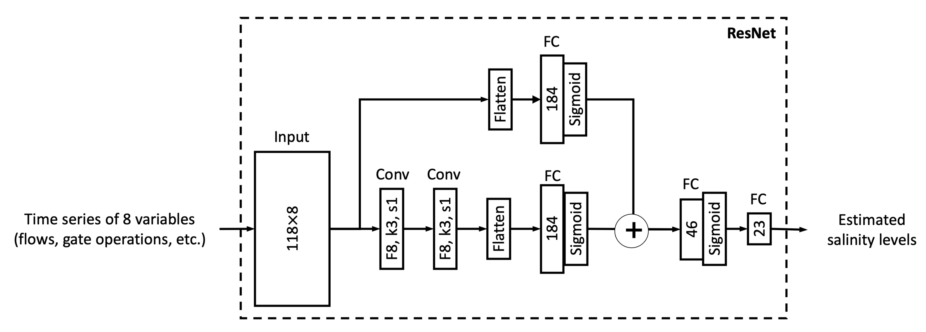
2.2. Machine Learning Models

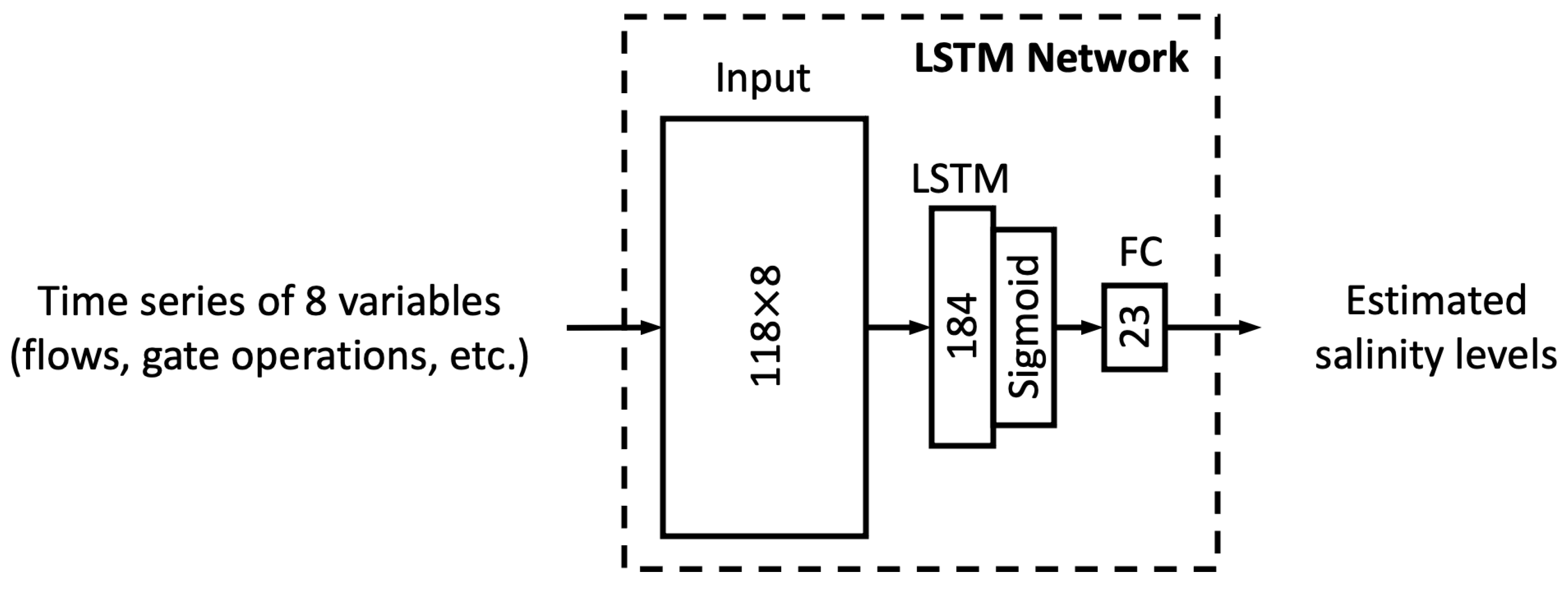
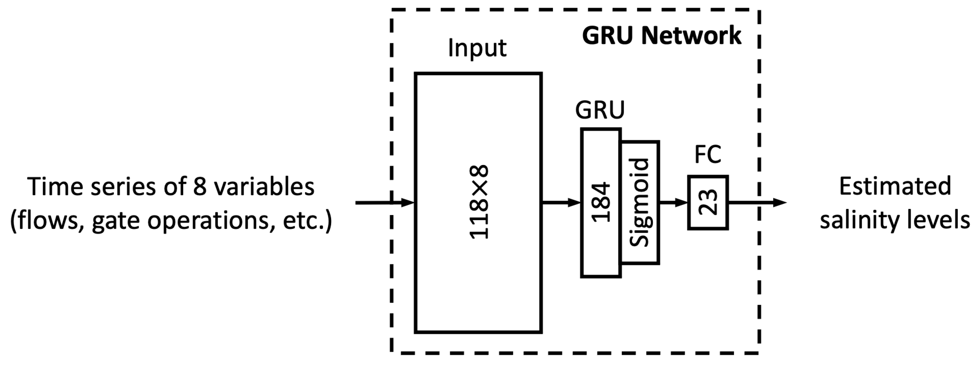
This study explores the use of six different ML models in a multi-task learning framework (i.e., one ML model for all study locations). Four of them were investigated in our previous study [29] where they were trained and tested using noise-free salinity simulations rather than real-world field observations of salinity. The current study adopts the same architectures applied in [29]: a multi-layer perceptron (MLP) network, a residual network (ResNet), a long short-term memory (LSTM) network, and a gated recurrent unit (GRU) network. The workflow of each of these four models is provided in Appendix C. These models are briefly described as follows. For detailed explanation on them, the readers are referred to [29].
The MLP model consists of one input layer, two fully connected (FC) hidden layers, and an output layer. The number of neurons in the two hidden layers is the number of study locations multiplied by 8 and 2, respectively. The input time series are pre-processed before being sent to the MLP model, which will be discussed in detail in Section 2.3. Results in [29] show that an MLP model achieves satisfactory salinity estimates, but the pre-defined input pre-processing procedure can still lead to unavoidable information loss in the input data. To improve the performance of the MLP model, a ResNet [55] model is developed by adding a shortcut side path including two convolutional layers and a FC layer to the vanilla MLP model to skip the pre-processing step so that the temporal information in the inputs is preserved. In addition to MLP and ResNet, Ref. [29] also explored two recurrent neural networks (RNNs): GRU and LSTM. RNNs maintain a memory internally in order to preserve essential temporal information from the inputs and have also achieved great success on time series analysis and processing tasks. GRU is one type of the popular RNN architecture designed for processing sequential data, which consists of a reset gate and an update gate connected to its hidden state. Similar to GRU, LSTM models keep a hidden state, which is the short-term memory, while storing an additional cell state, also known as long-term memory. Following [29], in the current study, we set the numbers of neurons in FC layers in ResNet, or numbers of RNN units in LSTM and GRU models equivalent to the numbers of neurons in the baseline MLP model.
In addition to these four models, we devise two novel architectures: Res-LSTM and Res-GRU. LSTM and GRU models applied in [29] are beneficial for time-series-related tasks, as they are capable of keeping track of memory when processing sequential inputs in an iterative manner. However, they have two major drawbacks. Firstly, they usually appear as complex models with more parameters than non-RNN models such that sufficient memory can be retained. Secondly, as the subsequent cell states in GRU and LSTM depend on the previous ones, computations cannot be processed in parallel, making them run slower than MLP or ResNet by design.
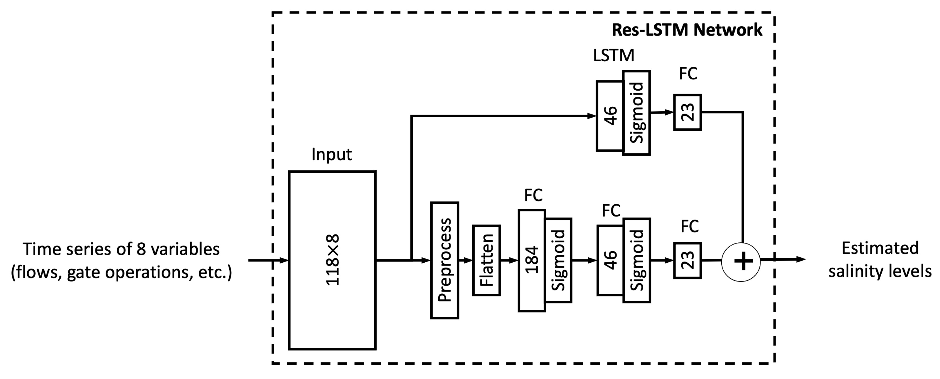
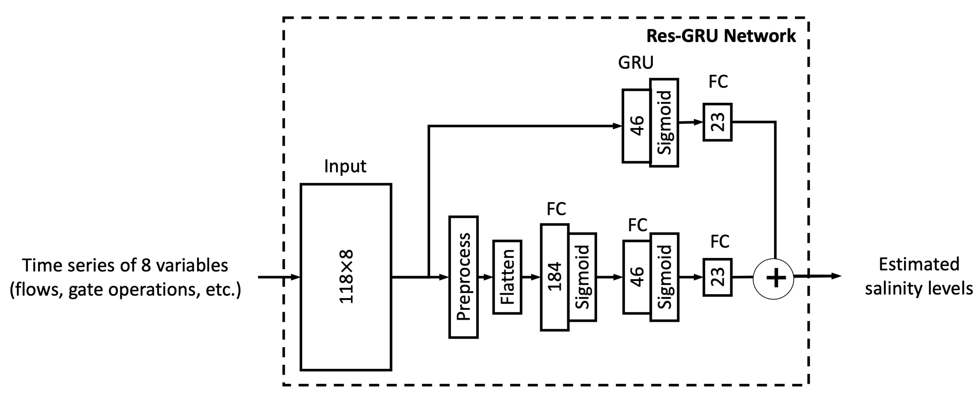
In order to address these two issues, inspired by the shortcut design in ResNet, we propose the Res-LSTM and Res-GRU models, which are less complex than the baseline LSTM or GRU models, respectively. According to our previous work [29], a vanilla MLP model already yields satisfactory results. Therefore, we directly use the MLP model as the main branch in Res-LSTM or Res-GRU models, as illustrated in Figure 3 and Figure 4 below. The numbers of neurons, 184 and 46, of the two hidden FC layers in the main branch are identical to those in the original MLP baseline model. In addition, we add the shortcut connection, consisting of a single LSTM or GRU layer, such that the error, or the residual, between the ground truth and the outputs of the MLP model can be captured. Taking advantage of the powerful MLP baseline model, we can reduce the complexity of the LSTM or GRU layer in the shortcut path in comparison with the baseline LSTM or GRU models. Here, we arbitrarily pick the number of units in the LSTM or GRU layers to be 46, which is equivalent to the number of neurons in the second hidden layer of the MLP baseline model. The number of parameters of the six aforementioned models can be found in Table 2.
The LSTM or GRU layers in the shortcut branch takes the time series of the eight input variables as inputs. At each of the 118 daily time steps in inputs, the RNN layers process one set of daily values of the eight input variables to update their hidden state and/or cell state accordingly. At the final 118-th daily time step, the LSTM or GRU layer outputs its final hidden state, which is supposed to fit the error or residual defined above. When applying the Res-RNN models for salinity forecasting, we simply shift the target salinity forward by a given lead time such that the outputs generated by these Res-RNN models represent the salinity values in the future.
As can be seen in Table 2, the Res-LSTM and Res-GRU use fewer parameters than their corresponding vanilla LSTM and GRU models. Meanwhile, in theory, they ought to outperform the vanilla MLP model since the shortcut side branch can learn to compensate for residual errors of the MLP main branch. Additionally, they need shorter training times.

2.3. Input Preprocessing

The inputs for the proposed ML models are generated using the same pre-processing strategy as introduced in [29]. Specifically, given the long memory of the Delta, where flow and operations in the past several months have lagged impacts the current salinity conditions [26,27,28], we aggregate 118 antecedent daily values of each of the 8 input variables into 18 values per input variable. These 18 values consist of one measurement from the current day and 7 daily measurements from the most recent 7 preceding days, together with 10 non-overlapping 11-day averages of the prior 110 days.
We use bold symbols for vectors and regular symbols for scalars. We utilize superscript to represent vector indices and subscript to represent input and output variable indices. For instance, x i t stands for the i-th input variable on day t. We write the mean of the i-th input variable computed based on a time frame from day t 1 to t 2 , with t 1 < t 2 , as x i t 1 t 2 ¯ , where
x t 1 t 2 ¯ = 1 t 2 t 1 + 1 t = t 1 t 2 x i t
We apply linear min-max normalization on the input time series and the salinity at each study station to the range of [0, 1]. That means that for each input feature or each salinity sequence at each station over the 20-year time span, the minimum value is transformed to 0, while the maximum value is transformed to 1. To be more specific, taking x i t , the i-th input variable on day t, as an example, it is normalized according to Equation (2), where T is the total number of samples.
x ^ i t = x i t ( min k = 1 , , T x i k ) ( max k = 1 , , T x i k ) ( min k = 1 , , T x i k )
The inputs for the proposed MLP network used to estimate reference salinity levels on day t consist of 8 daily values x ^ i t , , x ^ i ( t 7 ) ( 1 i 8 ), and 10 average values x ^ i ( t 8 ) ( t 18 ) ¯ , , x ^ i ( t 107 ) ( t 117 ) ¯ computed on 10 successive 11-day sliding windows, without overlapping, on the prior 110 days. The 18 processed values of each input variable make up the 8 × 18 = 144 inputs parameters for the MLP network. This pre-defined pre-processing method reduces the dimension of the input vector and avoids unnecessarily increasing the complexity of proposed MLP model, as well as preserving historical memory in the input time series.
For the proposed ResNet, LSTM, GRU, Res-LSTM and Res-GRU models, as they are designed to be more complex than the MLP model and require more detailed information from the input data, we directly input the 118 daily values x ^ i t , , x ^ i t 117 of each input variable x ^ i ( 1 i 8 ).
Model inputs are prepared in the same way as discussed above. For salinity estimation on day t, namely, the case where lead time t l = 0 , the salinity levels observed on day t at each of the 23 monitoring stations, depicted as y k t , where k = 1 , 2 , , 23 is the index of the monitoring stations, are set as target outputs during training or testing.

2.4. Forecasting Setup

In our previous work [10,29], we focused only on the investigation of same-day salinity estimation (i.e., the lead time is zero). In practice, forecasting near-term salinity is critical to informing real-time water management decision making. In this work, we extend the scope of proposed Res-LSTM and Res-GRU models to salinity forecasting up to 14 days into the future (lead time equals 14 days). Specifically, one ML model is trained for each lead day. A total of 14 Res-LSTM models and 14 Res-GRU models are developed.
For salinity forecasting on day t with a lead time of t l , we perform the following pre-processing steps:
Step 1:
We prepare model inputs the same way as discussed in Section 2.3, which consists of x ^ i t , , x ^ i ( t 7 ) ( 1 i 8 ) and x ^ i ( t 8 ) ( t 18 ) ¯ , , x ^ i ( t 107 ) ( t 117 ) ¯ .
Step 2:
We formulate the target output values by shifting the salinity values forward by t l days, represented by y k t + t l , k = 1 , 2 , , 23 .
In this way, after training, the models shall be capable of predicting daily salinity levels at the 23 monitoring stations ahead of time by t l days.
In the remaining of the paper, ML models trained with a lead time of zero ( t l = 0 ) are referred to as “salinity estimation” models, while models trained with a lead time of greater than or equal to 1 ( t l 1 ) are referred to as “salinity forecasting” models. It is worth noting that forecasting models here differ from models applied in real-time forecasting operations which use forecast model inputs to drive the model and generate forecasts. The forecasting models developed for each lead time (i.e., day 1 through day 14 into the future) in the current study use purely historical data up to the lead time of zero.

2.5. Evaluation Metrics

The proposed models are trained with the Adam optimization algorithm [56] based on the widely used mean squared error (MSE) loss function. Four statistical evaluation metrics, consisting of the square of the correlation coefficient ( r 2 ), bias, root mean standard deviation ratio (RSR), and the Nash–Sutcliffe efficiency coefficient (NSE), are employed to assess the ML model performance. Each of the four metrics evaluates the modeled salinity performance from a different perspective: r 2 quantifies the strength of the linear relationship between modeled salinity and the target salinity; percent bias indicates whether the models over- or underestimate the salinity; RSR is a standardized representation of the root mean squared error (RMSE) between model outputs and targets; and NSE compares the predictive capacity of the models with the global mean of target sequences. For r 2 and NSE, a value close to 1 indicates desirable model performance. For percent bias and RSR, a value close to 0 designates good model performance. Table 3 provides detailed descriptions and definitions of these five metrics. Here, S represents the salinity sequence, S ¯ indicates the overall average value of the salinity levels S, and the subscripts A N N and O b s e r v e d indicate ANN-estimated and observed salinity, respectively.

2.6. Implementation Details

Our experiments are carried out on a public platform: the Google Colaboratory. Hyper-parameters such as batch size, learning rate and numbers of epochs may affect model performance. The authors of a previous study [57] optimized some hyper-parameters in the backpropagation neural network (BPNN) architecture, including the number of nodes in the model, the learning rate, and number of epochs. In a different manner, we used a constant small learning rate of 0.001 with the Adam optimizer [56] to train our models and stopped training if the mean squared error (MSE) on the test set did not decrease for 50 epochs. In addition, to prevent overtraining, we limited the maximum number of epochs to 5000. In this way, we did not have to specifically optimize the learning rate or the number of epochs.

3. Results

This section presents the results of the proposed ML models, particularly those two novel models. Firstly, the training and testing performance of all six models is scrutinized in terms of the skill metrics described in Section 2.5 as well as visual inspection of modeled salinity against the corresponding observations. Next, the forecasting capability of the two proposed novel models is examined. Finally, model performance is evaluated on the hourly time step.

3.1. Model Performance on the Daily Scale

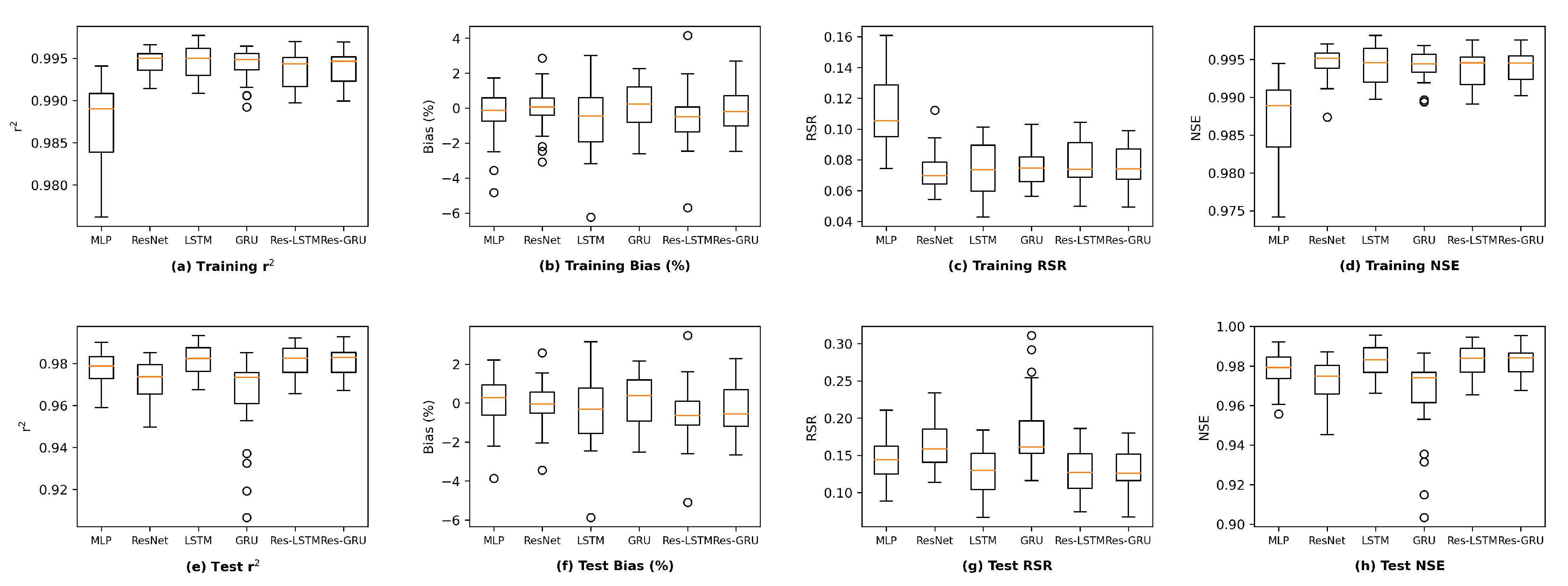
Figure 5 illustrates the performance of the two exploratory ANNs, Res-LSTM and Res-GRU, in comparison with the original four basic networks, MLP, ResNet, LSTM, and GRU, in terms of the four study metrics ( r 2 , Bias, RSR, and NSE). The figure reveals that the two new models (Res-LSTM and Res-GRU) have satisfactory performance. Specifically, the training results in Figure 5a–d indicate that both Res-LSTM and Res-GRU outperform MLP, while being at a similar level with ResNet, LSTM, and GRU. The former is most likely due to the learning compensation of the shortcut side branch from Res-LSTM and Res-GRU compared to MLP. The latter suggest that the new and simpler structures of Res-LSTM and Res-GRU could successfully achieve similar performance to their more complex counterparts, LSTM and GRU. Meanwhile, the test results in Figure 5e–h suggest that Res-LSTM and Res-GRU yield better or similar results to the four original models. All in all, Res-LSTM has a slight edge over other models, as it has slightly more desirable metrics. Simulations from Res-LSTM are further examined and compared with the observed salinity in different ways.
Figure 6 shows the corresponding exceedance probability curves and daily time series plots of Res-LSTM simulations compared with the observed data at selected locations. Both types of plots demonstrate that the simulations mimic the target observed salinity very well, with the latter showing capture of the temporal pattern and magnitude in general. Another notable pattern is that, despite the marginal discrepancies in the full salinity spectrum between the two models, time series plots reveal that Res-LSTM slightly underestimates high salinity, especially for RSAC092 and RSAN018.
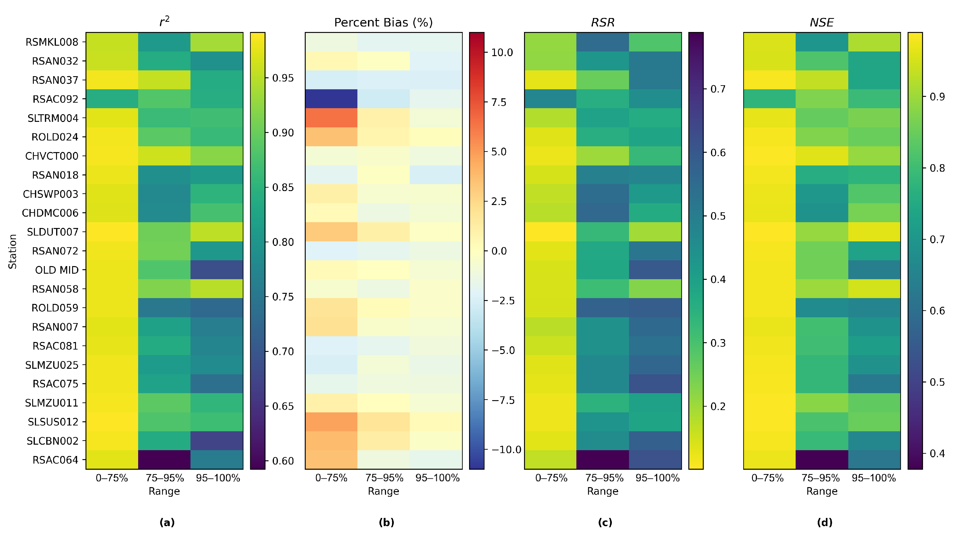
Figure 7 shows the statistical metrics for each study location, calculated at three ranges, illustrating the performance of the Res-LSTM model compared to observed data on a daily time step. For metrics r 2 , NSE, and RSR, “yellow” indicates satisfactory performance. For the percent bias metric, shaded blue and orange represent underestimation and overestimation, respectively. Overall, model performance is most satisfactory when the salinity is in the low–middle range (0–75%) and decreases with high (75–95%) and extremely high (95–100%) salinity ranges. Several notable observations are further discussed below.
Performance at location RSAC092 (Sacramento River at Emmaton) is lower in the low salinity range but is consistent with the other locations in the high and extremely high ranges. Despite the departure from the other stations, overall, r 2 , NSE, and RSR for RSAC092 are acceptable. The Res-LSTM model underestimates salinity in the low–middle range, where the percent bias is −11%. This is because the Res-LSTM often estimates zero EC at Emmaton, but this generally does not occur in the observed data. At location RSAC064 (Port Chicago), r 2 , NSE, and RSR are acceptable in the low–middle and extremely high ranges, but less satisfactory under the high range. The Res-LSTM is less able to capture the salinity variability at Port Chicago under the high range, but the percent bias is acceptable and consistent with other locations. At locations in the Suisun Marsh (SLMZU011, SLSUS012, SLCBN002), the Res-LSTM tends to overestimate salinity, especially in the low–middle range.
In short, the novel Res-LSTM and Res-GRU models can satisfactorily estimate salinity at the locations studied, while achieving similar or better performance compared with their more complex LSTM and GRU counterparts. Generally, performance is best at stations with lower median salinity and variability and degrades at stations with higher salinity and variability. The combination of a simpler architecture paired with comparably good performance to vanilla LSTM and GRU models indicate that the new models show promise in estimating Delta salinity on a daily time step.

3.2. Forecasting Performance

Figure 8 compares the forecasting performance of the Res-LSTM model during the training (Figure 8a–d) and test (Figure 8e–h) runs, using box and whisker plots for four types of metrics consisting of r 2 , percent bias, RSR, and NSE. Each plot includes one box and whisker for each lead time evaluated. The statistical meaning of the boxes, whiskers and circles is the same as in Figure 2.
Generally speaking, model performance declines smoothly as the lead time increases, and all the metrics are within a reasonable range. Even with a lead time of 14 days, the Res-LSTM model predictions are satisfactory. For all lead times evaluated under training and testing, NSE is above 0.94, r 2 is above 0.95, and percent bias centers around zero percent, indicating excellent predictive performance without a tendency to systematically underestimate or overestimate.
Figure 9 shows the corresponding performance of Res-GRU models based on four criteria ( r 2 , bias, RSR, and NSE) in two rows. The first row (Figure 9a–d) and the second row (Figure 9e–h) display the performance of Res-GRU for training and test datasets, respectively. As a performance indicator for ML algorithms, results of the test dataset (Figure 9e–h) indicate that the nowcasting (forecasting with 0 lead time) model has the best performance, and the forecasting model’s accuracy decreases when the lead time increases, which is reasonable for every forecasting model. However, the forecasting model with 6 and 12 days lead time does not follow this pattern, and the forecasting model with a 6-day lead time provides the worst performance but still is satisfactory ( r 2 and NSE are high, while RSR and bias are low). This suggests that the historical data up to lead time 0 alone may not be ideal to forecast these two days for the Res-GRU model. Overall, all the metrics are within a reasonable range. For all lead times evaluated under training and testing, NSE is above 0.94 and r 2 is above 0.94, indicating satisfactory performance overall. The percent bias metric indicates higher variability than the Res-LSTM predictions (Figure 5) but does not show a clear systematic bias toward underestimation or overestimation.
All in all, for all lead times considered, Res-LSTM and Res-GRU can forecast salinity levels at all study locations with satisfactory performance. Model performance generally decreases as the lead time increases.

3.3. Model Performance on the Hourly Scale

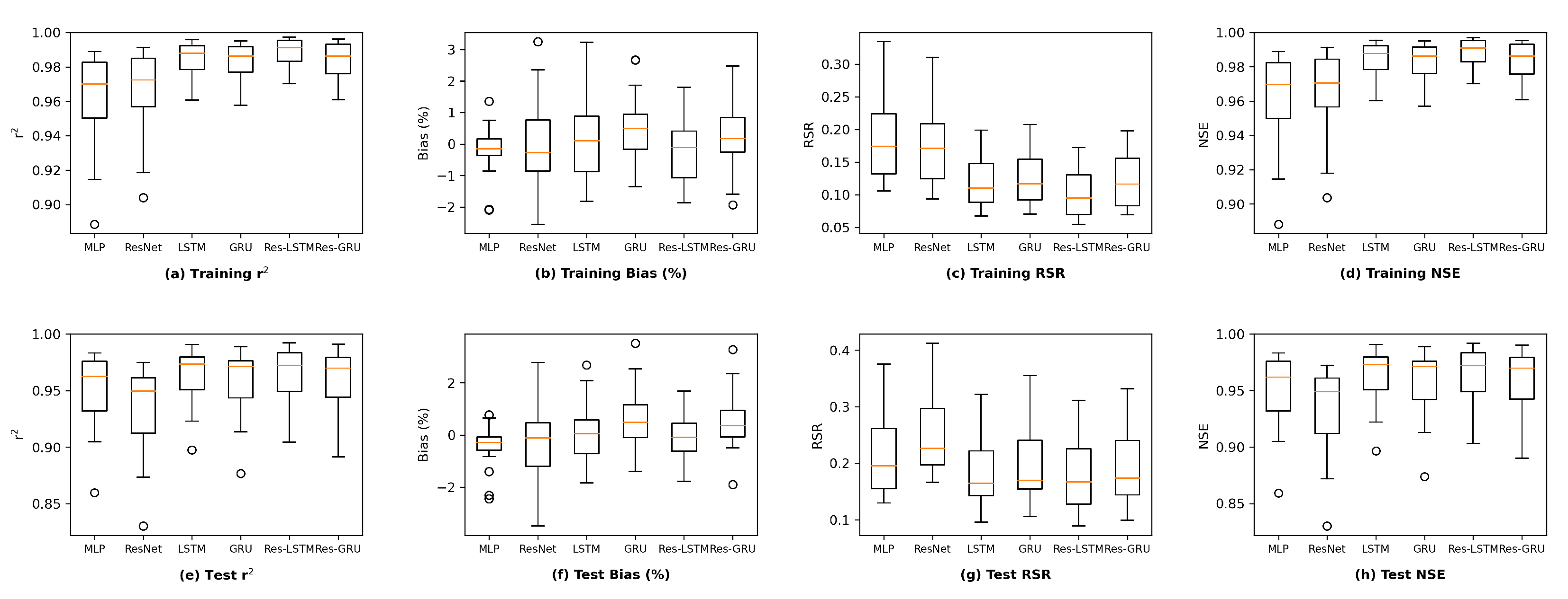
The results presented so far are all trained and tested using daily salinity data aggregated from the hourly observations of salinity. In this sub-section, the six ML models proposed are trained using the hourly observations directly though the input data supplied to the models and are still on the daily scale. Figure 10 compares the performance of these models during the training (Figure 10a–d) and test (Figure 10e–h) runs, using box and whisker plots for four types of metrics consisting of r 2 , percent bias, RSR, and NSE. Each plot includes one box and whisker for each model evaluated. Based on these metrics, the Res-LSTM model generally outperforms all the other ML models tested during training and test runs. On average, Res-LSTM has the highest r 2 and NSE. It also has the lowest bias and RSR for both training and testing. The performance of Res-GRU is close to but not as ideal as that of Res-LSTM. In contrast, ResNet has slightly inferior performance compared to other ML models, followed by MLP. Compared to their counterparts on the daily scale (Figure 5), the skill metrics r 2 , RSR, and NSE are notably inferior, indicative of stronger performance on the daily (versus hourly) scale for all six models.
Figure 11 shows the corresponding exceedance probability curve and hourly time series plots to evaluate the performance of Res-LSTM at six selected locations in the Delta. In general, the differences between model simulations and the corresponding observations are marginal. However, the time series subplots indicate that the Res-LSTM models slightly underestimate the peak values at some of these specified locations. Nevertheless, the plots show remarkable similarity between models and observations, and the Res-LSTM model can skillfully capture the temporal pattern of observed salinity. Comparing Res-LSTM performance on the daily scale (Figure 6) versus the hourly scale (Figure 11), the metrics associated with the daily scale are generally superior. In particular, the r 2 and NSE are slightly higher while the RSR is generally lower on the daily scale. This is also observed for other models as illustrated in Figure 5 and Figure 10.
As in Figure 7, Figure 12 shows heatmaps which summarize the performance of the Res-LSTM model with hourly time steps using the statistical metrics r 2 , percent bias, RSR, and NSE for each study location. In general, model performance is the most satisfactory for salinities in the low–middle range across most stations, but lower for the high and extreme high ranges. Compared to the daily time step simulation results in Figure 7, the metrics associated with the hourly time step are inferior for most locations. The detailed values of all four study metrics on both daily and hourly scales are provided in the Appendix D.
In a nutshell, all six proposed models can achieve satisfactory performance at a finer hourly scale, and Res-LSTM slightly outperforms the other five. The differences between model simulations and the corresponding observations are small on average. The performance of Res-LSTM is highest in the low–middle range, but relatively lower for the high and extreme high ranges. Compared to their counterparts on the daily scale, the ML models on the hourly scale generally have slightly degraded performance.

4. Discussions

This section first discusses the overfitting potential of the ML models proposed in the study. Second, the performance of a selected ML model is compared with that of the process-based model DSM2, which is widely used to inform water operations in the Delta. Next, the section discusses the scientific and practical implications of the study, followed by discussions on study limitations and planned future work.

4.1. Overfitting Potential versus Model Complexity

Overfitting happens when a ML model picks up the details, including noise, and fits exactly on the training data but does not generalize well on unseen data [58,59]. Overfitting is a central problem in the field of data-driven ML, as it negatively impacts the model’s generalization performance on new data. Overfitting is more likely to occur when a model’s structure is too complex for the task. To avoid this problem, the number of neurons or units in the layers need to be determined carefully.
In this study, we proposed six different ML models. In this sub-section, we explore the relationship between model complexity and salinity estimation performance by reducing the number of neurons in the hidden layers of each model. For the MLP, ResNet, Res-LSTM and Res-GRU models, we adjust the number of neurons in two fully connected hidden layers in the main branch, depicted by n 1 and n 2 , respectively. In addition to the original settings, where n 1 = 184 and n 2 = 46 , we pick four combinations, including { n 1 = 138 , n 2 = 46 } , { n 1 = 92 , n 2 = 46 } , { n 1 = 46 , n 2 = 46 } and { n 1 = 46 , n 2 = 23 } to build four simplified versions as well as five additional combinations of { n 1 = 184 , n 2 = 92 } , { n 1 = 184 , n 2 = 138 } , { n 1 = 184 , n 2 = 184 } , { n 1 = 368 , n 2 = 92 } , and { n 1 = 368 , n 2 = 184 } that lead to complicated versions for each of the four models. For the vanilla LSTM and GRU models, we change the number of units in the recurrent layer from 184 units to 322, 276, 230, 138, 92, 46 or 23 units. A detailed list of the number of parameters in these models can be found in Table A10 and Table A11 of Appendix E.
We plot the model performance (in terms of the average value of each evaluation metric across the 23 study locations) versus model complexity (in terms of number of parameters) in Figure 13. In general, model performance improves as complexity grows. In both the training and test plots of r 2 , RSR and NSE, MLP models show the best complexity–performance trade-off. Namely, the MLP model can achieve a comparable performance with other models with a relatively smaller number of parameters. However, during the grid search process when designing these models, we observed that the MLP model hits a performance plateau earlier than other models, namely, the test performance stops improving, even if we keep increasing the number of neurons in its hidden layers. In contrast, the ResNet model gives the worst complexity–performance trade-off because the extra FC hidden layer in its shortcut branch adds a large number of parameters to the model. Comparing the vanilla RNNs (i.e., LSTM and GRU) and their corresponding Res-RNN models, we see that the simple RNN module in the residual path ensures a satisfying model performance while bringing down the complexity.
In brief, model performance improves as the complexity grows but both training and test performance will hit a plateau at some point. No obvious overfitting was observed during our exploration, suggesting that the proposed models are not over-parameterized and well-trained.
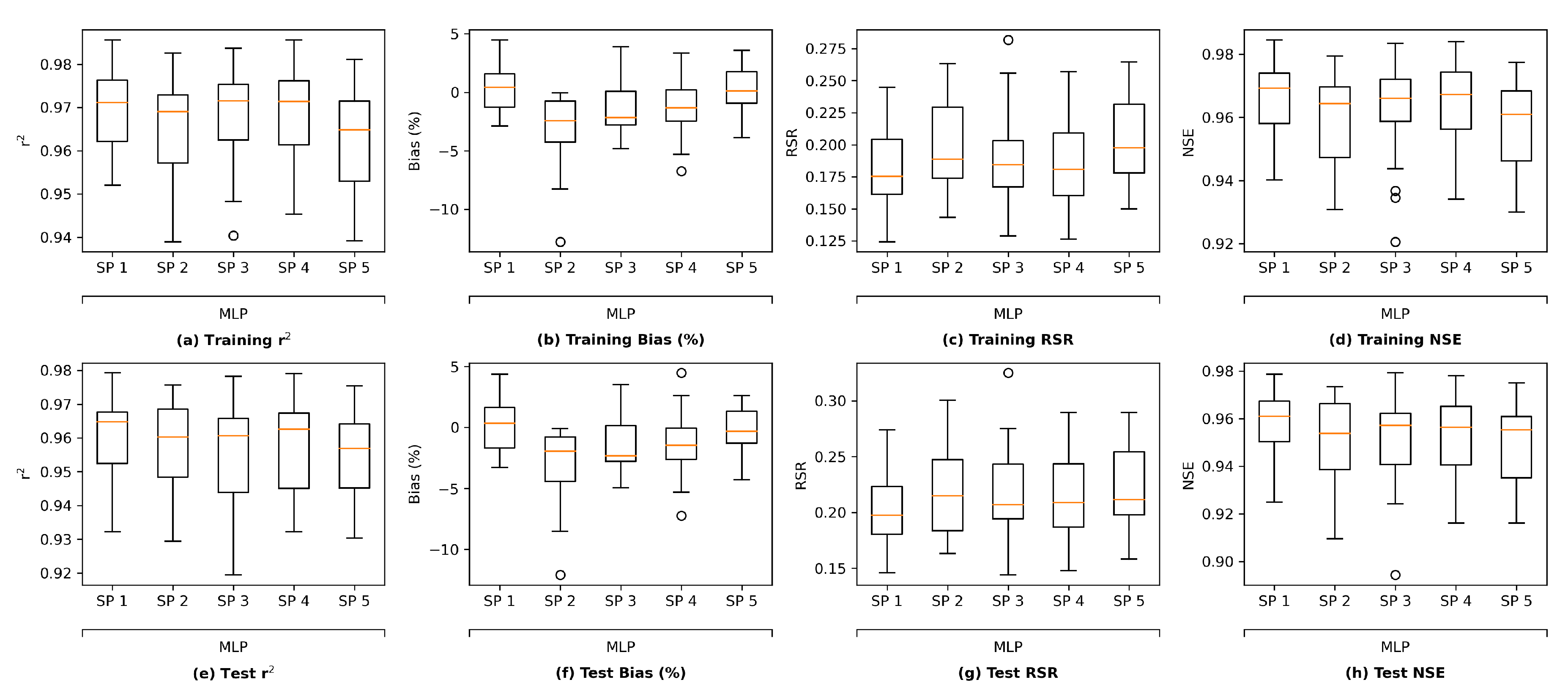
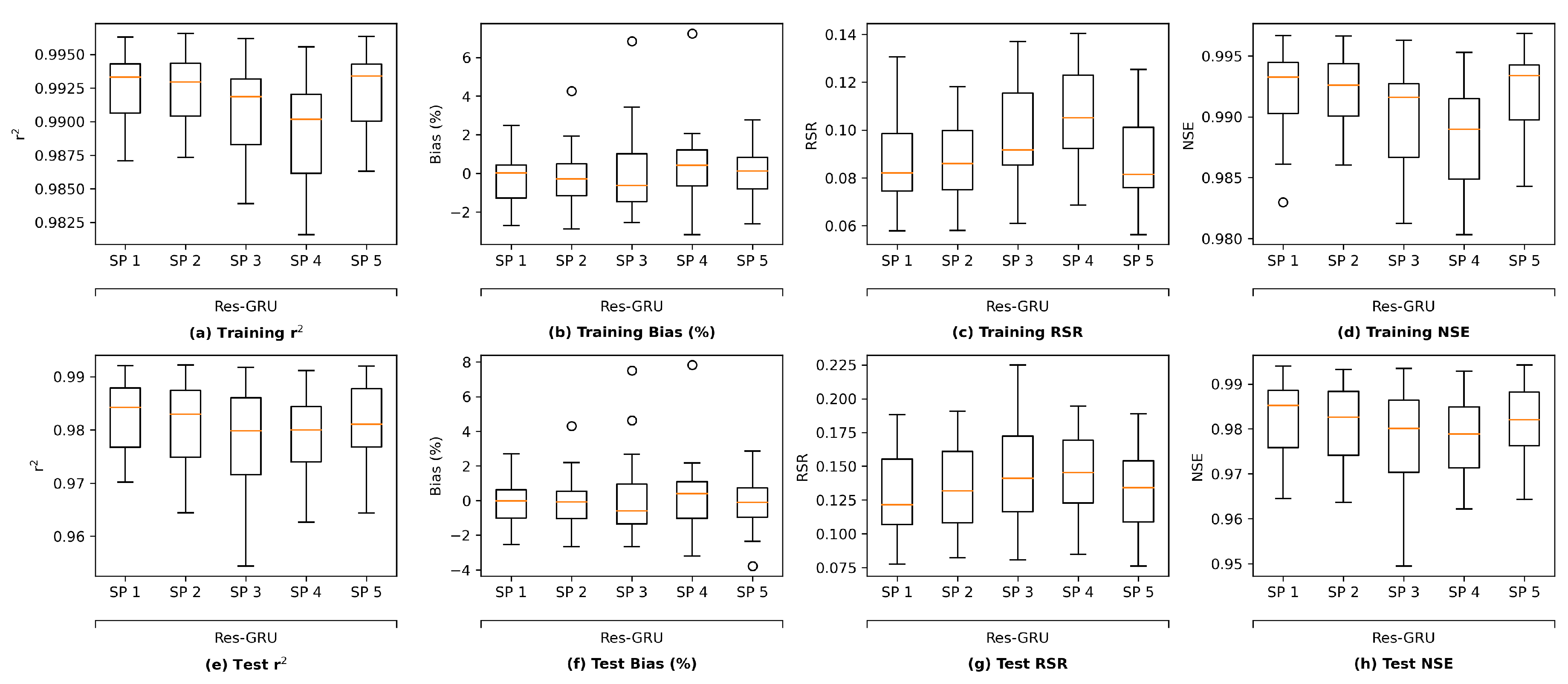
It is worth noting that there are other methods that can be applied to assess the overfitting potential of machine learning models. The current study briefly explored two of those methods, namely data distortion and cross validation for demonstration purposes. The results (Figure A5Figure A8 in Appendix F) also indicated that no evident overfitting was observed.

4.2. Comparing with a Process-Based Model

It is shown in Section 3 that the proposed ML models in this study, particularly the novel Res-LSTM and Res-GRU models, can simulate and predict real-world salinity in the Delta well. Traditionally, process-based models, including the operational hydrodynamics and water quality model DSM2, have been applied to simulate and predict the spatial and temporal variations of the salinity across the Delta. It is imperative to assess the performance of these ML models against that of the operational process-based models. For illustration purposes, this sub-section compares simulations from the Res-LSTM model and its counterparts from DSM2.
The comparison is conducted by means of both visual inspection and evaluating statistical metrics. Figure 14 shows the comparison among time series plots of the measured DSM2-simulated and Res-LSTM-simulated EC data at six selected key stations. Four study metrics ( r 2 , Bias, RSR, NSE) of both sets of models are also displayed side-by-side to conduct quantitative comparison. The corresponding comparison for all 23 study locations is provided in Appendix G. Both simulations mimic the target filed measurements of salinity very well via visually inspecting the time series plot. The overall biases of both models are generally small. For Res-LSTM, the absolute bias ranges from 0.3% to 4.6%. The r 2 , RSR and NSE values of Res-LSTM are notably better than their counterparts of DSM2 for all six locations. Collectively, these observations indicate that Res-LSTM yields comparable or more desirable salinity simulations compared to the operational DSM2 model.
Nevertheless, it should be pointed out that DSM2 can generate salinity simulations not only at the 23 study locations, but at all channels across the Delta. The ML models proposed in the study can only be applied to study locations where they have been trained, and thus are not meant to be substitutes of process-based models, including DSM2.

4.3. Implications

This study has important scientific implications. Firstly, the study exemplifies the feasibility of applying ML, particularly deep learning models, as a new scientific exploratory tool to tackle a complex problem. Secondly, this study proposes two novel deep learning models (i.e., Res-LSTM and Res-GRU) that have never been explored before. These novel models can be applied to simulate other variables, including water temperature, suspended sediment, dissolved oxygen, and other water quality variables, that are important to guide water management practices in the Delta. Thirdly, this study illustrates the forecasting capability of newly developed deep-learning models. Effective and efficient forecasting models are valuable tools that can guide real-time operations in light of forecast near-term salinity conditions.
There are also important practical implications of this study. The study demonstrates that the proposed ML models are capable of generating desirable salinity simulations and predictions even on the hourly scale. The overall absolute biases are generally less than 5%. The correlation coefficients, RSR, and NSE values are generally satisfactory. They are either comparable or superior compared to the corresponding metrics of the DSM2 model. In addition to accuracy, the proposed ML models are also of high efficiency. DSM2 runs can take hours depending upon the simulation period length [28], while the runtime for trained ML models for the same inputs is measured in seconds. This is particularly appealing, for instance, for real-time operations which require quick turn-around time and also studies that require running multiple scenarios during the historical period.

4.4. Limitations and Future Work

Despite those scientific and practical implications, this study has several limitations. First of all, the current study randomly splits the dataset into a training subset and a test subset. Though random split of training/testing in not uncommon in ML studies in the Delta [2,10,26,27,28,54], there are other data-split methods available. Ref. [29] examined chronological split and manual split and found that the performance of the random split method yielded improved results over the other methods. Since the observed data are about one-third shorter than the simulated data used in [29], this study did not employ the chronological/manual methods. In our future work focusing on larger datasets, we will explore chronological split and manual split methods. In addition, explainable artificial intelligence (XAI) is an active research area [60]. There have been a number of XAI approaches developed. In our future work, we plan to explore various XAI approaches, including the gradient-based method [61] and the backpropagation-based method [62], and the input variable sensitivity analysis [57], and conduct in-depth investigation of the importance of different inputs features in different regions and locations in the Delta.
This study used eight empirical variables as input features to the proposed models. They were shown to yield desirable salinity estimation at the study locations. However, other variables, including precipitation and wind speed, also influence the circulation and mixing of freshwater and sea water and thus affect the salinity level in the study area. In our future work, we will also explore the impacts of additional input features on the ability of the proposed models to estimate Delta salinity.
In this study, the ML models are trained and tested on historical time series. The selected range of data may not capture potential hydrologic extremes or increased water use. Climate change is expected to cause larger storm-driven streamflow and altered runoff timing [63]. In addition, in the coming decades, municipal, industrial and agricultural water demand in California is projected to increase from increasing urbanization and changing agricultural practices [64]. The models trained on historical data, therefore, will not be exposed to the range of inflows and operational constraints resulting from potential future conditions. Additionally, the ML models are trained using data from 23 study locations and can thus only be applied to those study locations. In the future, we will explore generic ML models capable of generating salinity estimates at locations they are not trained upon.
Exclusively using the historical record for training may also introduce shortcomings when conducting long-term planning studies, as the training dataset is not modified beyond the scope of historical operational considerations. In real-time operations and planning, measures such as emergency barriers and temporary operational regimes may be implemented to manage flow and salinity. Operational measures include emergency temporary barriers [65] to manage salinity intrusion and maintain acceptable water quality at pumping locations. The historical time series reflects limited use of emergency operational measures and does not consider the operation of the Suisun Marsh Salinity Control Gates (SMSCG). The limitations associated with using a historical dataset during training will be addressed in future work, where the model will be trained using synthetically augmented datasets.
Data augmentation is a technique to generate synthetic data for model training, which incorporates an enlarged and diversified dataset to better represent extreme conditions and possible future conditions. In our ongoing preliminary tests, we use DSM2 historical simulation as the baseline, then apply several modifications, including (1) scaling the magnitude of major boundary flows; (2) temporally shifting major boundary flows; and (3) changing operations of key Delta structures, such as operable gates. All of the above aim to reduce overfitting and thus improve the generalization ability of the trained neural networks. Another benefit of data augmentation is that it can provide sufficient time series for chronological split training to bypass the limit of random split method.
In another follow-up work, we plan to explore the physics informed neural network (PINN), a cutting-edge neural network algorithm which can embed the knowledge of physical laws into data training. Most of the physical laws governing the dynamics of a system can be described by partial differential equations (PDEs). PINN adds the underlying PDE of the dynamics directly into the loss function of the neural network [66,67]. For our study, we plan on implementing PINN with the one-dimensional advection–dispersion equation for salinity transport [14,68].
PINN can be viewed as a regularization limiting the space of admissible solutions, through adding the prior knowledge of general physical laws in the training of neural networks. Its benefits include increasing the correctness of the function approximation, facilitating the learning algorithm to capture the right solution, generalizing well, even with a low amount of training examples, and providing a meshfree alternative to traditional approaches. PINN could also be viewed as a paradigm that bridges the gap between the process-based models, which are developed from the known PDEs of the dynamics, and the machine-learning models, which are driven purely by existing data. By integrating the best of both methods, namely, the physics information of the process-based models and the training data employed in the machine-learning models, PINN could learn the underlying solution of the dynamics more accurately and more efficiently.
Moreover, this study explored the forecasting capability of the two proposed novel ML models using historical data up to the forecast time only. The main reason is that we do not have forecasted input variables available. It is expected that the performance of the ML models would be even more satisfactory should forecasted model inputs be used to drive the models. In a follow-up study, we plan to collect archived forecasted inputs and salinity data from real-time operations, and develop ML models based on them, and test the trained model in a hindcasting mode.
Lastly, we are developing an interactive dashboard to integrate and visualize our modeling results. It is designed as a front-end to the trained neural network model engine, allowing users to customize data inputs, run the ANNs, and query results. The proposed dashboard could generate a visualization of the time-series output and their proposed metrics for all the specified locations across the Delta. This tool could facilitate management decisions in historical, real-time, and forecast applications.

5. Conclusions

Built upon the success of relevant previous studies that explored machine learning applications in salinity modeling in the Delta, this study develops two novel deep learning models and applies them in both salinity simulation and prediction as well as on a finer hourly time scale that had never been investigated before. The study shows that the novel models proposed can effectively simulate and predict salinity at all study locations across the Delta. In addition, compared to traditional process-based models, the proposed models run significantly faster once trained. Their effectiveness and efficiency make them viable supplements to operational process-based models in terms of providing salinity estimates to inform both real-time and long-term water management and planning practices.

Author Contributions

Conceptualization, P.S., Z.B., Z.D. and M.H.; Data curation, B.T., R.H., P.N. and Y.Z.; Funding acquisition, P.S.; Investigation, S.Q. and M.H.; Methodology, S.Q., M.H., Z.B., Z.D., P.S. and J.A.; Project administration, P.S.; Software, S.Q.; Validation, M.H., R.H., P.N. and Y.Z.; Visualization, S.Q., M.H.; Writing—original draft, S.Q., M.H., Y.Z., B.T., R.H., P.N. and J.A.; Writing—review and editing, Z.B., P.S., J.A., F.C. and D.M.R. All authors have read and agreed to the published version of the manuscript.

Funding

This research was funded by the California Department of Water Resources and the University of California, Davis grant number 4600014165-01.

Data Availability Statement

Data availability is described in Appendix A.

Acknowledgments

The authors would like to thank the editors and two anonymous reviewers for providing thoughtful and insightful comments that helped to improve the quality of this study. The views expressed in this paper are those of the authors, and not of the State of California.

Conflicts of Interest

The authors declare no conflict of interest.

Appendix A. Data Sources

Input data for the ML models along with observed salinity data are available at the following link: https://data.cnra.ca.gov/dataset/dsm2-v8-2-1 (accessed on 1 July 2022).

Appendix B. Summary of Datasets from Previous Studies

Table A1. Datasets applied in relevant previous studies.
StudyDataset
Rath et al. (2016) [2]The input features of this study are daily freshwater flow to the estuary, daily mean coastal water level, and the daily tidal range for water years 1922–2012. Labels are salinity data from nine locations collected from sensors in the Delta.
Chen et al. (2018) [28]In this study, the machine learning emulator is based on data generated using DSM2 (a process-based model) including its outputs at 17 locations for
10 scenarios (two decades each). The use of 10 scenarios is intended to augment the dataset to bound the range of possible water management operations. The study period 1990–2010 was strategically selected as it contains widely varying hydrology and is a period where the DSM2 model is well-calibrated.
Mosavi et al. (2018) [31]In this study, the authors examined studies that used field data from rain gauges and other sensing devices, including data from remote sensing technologies.
He et al. (2020) [10]The dataset includes a 24-year period (WY 1991–2014) of daily observed water stage at Martinez, Martinez salinity and the net Delta outflow.
Jayasundara et al. (2020) [26]Input features used are Northern flow, San Joaquin River flow, exports, Delta cross channel gate operation, net Delta consumptive use, tidal energy, and San Joaquin River inflow salinity at Vernalis. Labels include multiple sets of DSM2 simulated salinity data representing a range of operational conditions.
Qi et al. (2021) [27]The input features in this study are the same as Jayasundara et al. (2020) and the labels are DSM2-simulated salinity data at 12 locations.
Qi et al. (2022) [29]The input features of this study are eight inputs representing boundary flows or operating rules for Delta flow and salinity management. DSM2 simulated daily salinity at the 28 study locations during 1990–2019 is used as the training label dataset.

Appendix C. Diagrams of MLP, ResNet, LSTM and GRU Networks

Figure A1. Diagram of the MLP network from [29]. The number in the input layer denotes input shape and those in the subsequent FC layers represent the numbers of neurons of the layers.
Water 14 03628 g0a1
Figure A2. Diagram of the ResNet network from [29]. The number in the input layer denotes input shape and those in the FC layers represent the numbers of units/neurons of the layers. In the convolutional layers following the input layer, “f” denotes the number of convolutional filters, “k” denotes size of convolutional kernels and “s” denotes stride.
Water 14 03628 g0a2
Figure A3. Diagram of the LSTM network from [29]. The number in the input layer denotes input shape and those in the subsequent layers represent the numbers of units/neurons of the layers.
Water 14 03628 g0a3
Figure A4. Diagram of the GRU network from [29]. The number in the input layer denotes input shape and those in the subsequent layers represent the numbers of units/neurons of the layers.
Water 14 03628 g0a4

Appendix D. Detailed Values for Figure 7 and Figure 12

Table A2. Station-wise r 2 results of Res-LSTM at hourly time step with daily inputs.
r 2 0∼75%75∼95%95∼100%
RSAC0640.95290.59400.6464
SLCBN0020.97480.83340.6973
SLSUS0120.99090.88030.8518
SLMZU0110.99040.91110.9003
RSAC0750.97600.80080.7332
SLMZU0250.97770.77590.7619
RSAC0810.96230.79560.7625
RSAN0070.95680.82860.8028
ROLD0590.97280.72870.6267
RSAN0580.98090.91350.9437
OLD MID0.98170.87290.6846
RSAN0720.98600.89750.8538
SLDUT0070.99050.91560.9509
CHDMC0060.90640.63680.5679
CHSWP0030.93790.56950.4932
RSAN0180.94340.79810.7969
CHVCT0000.98940.97080.9405
ROLD0240.98600.89160.8700
SLTRM0040.90270.72000.8676
RSAC0920.58190.81650.8177
RSAN0370.98150.92210.8310
RSAN0320.87510.77130.7742
RSMKL0080.94840.73470.8541
Table A3. Station-wise percent bias results of Res-LSTM at hourly time step with daily inputs.
Bias0∼75%75∼95%95∼100%
RSAC0640.4684−2.8600−3.7659
SLCBN002−1.3600−0.8149−1.4523
SLSUS0120.2163−0.1661−0.6855
SLMZU011−0.2336−0.7538−1.0799
RSAC0751.5492−0.4411−0.8134
SLMZU0252.1184−0.0241−1.2001
RSAC0814.8211−0.0190−1.6114
RSAN007−2.6612−0.8044−2.3899
ROLD0590.0202−1.0317−1.8503
RSAN058−0.3692−1.2292−1.3330
OLD MID−0.0381−0.3858−0.9698
RSAN0720.5610−0.1732−0.1627
SLDUT0071.90580.8568−0.0001
CHDMC0061.3642−1.4991−3.1108
CHSWP0030.9000−1.1438−3.7689
RSAN0183.41332.5636−2.7383
CHVCT0000.54070.23390.1670
ROLD0240.51340.36750.1518
SLTRM004−1.2958−0.8454−1.6861
RSAC092−1.67661.0572−3.6682
RSAN0370.98730.2697−0.8718
RSAN032−1.3944−0.8808−4.2074
RSMKL0080.6971−0.2226−0.6141
Table A4. Station-wise RSR results of Res-LSTM at hourly time step with daily inputs.
RSR0∼75%75∼95%95∼100%
RSAC0640.22000.82970.8356
SLCBN0020.16090.45080.6052
SLSUS0120.09600.36600.4214
SLMZU0110.09810.31090.3718
RSAC0750.15820.48410.5874
SLMZU0250.15520.50960.5669
RSAC0810.20870.48880.5559
RSAN0070.22010.43630.5086
ROLD0590.16610.61130.7402
RSAN0580.13850.32380.2714
OLD MID0.13590.38560.6345
RSAN0720.11910.33830.4005
SLDUT0070.10230.30630.2214
CHDMC0060.32430.72880.8950
CHSWP0030.25980.82800.9698
RSAN0180.25410.51500.4731
CHVCT0000.10370.17540.2459
ROLD0240.12070.35090.3848
SLTRM0040.33910.61860.3708
RSAC0920.99230.44070.4853
RSAN0370.13920.29000.4270
RSAN0320.38600.52420.5271
RSMKL0080.23200.58440.4060
Table A5. Station-wise NSE results of Res-LSTM at hourly time step with daily inputs.
NSE0∼75%75∼95%95∼100%
RSAC0640.95160.31170.3017
SLCBN0020.97410.79680.6337
SLSUS0120.99080.86600.8224
SLMZU0110.99040.90330.8618
RSAC0750.97500.76570.6549
SLMZU0250.97590.74030.6786
RSAC0810.95640.76110.6910
RSAN0070.95160.80960.7413
ROLD0590.97240.62630.4521
RSAN0580.98080.89520.9264
OLD MID0.98150.85130.5975
RSAN0720.98580.88560.8396
SLDUT0070.98950.90620.9510
CHDMC0060.89480.46890.1990
CHSWP0030.93250.31450.0595
RSAN0180.93540.73480.7762
CHVCT0000.98920.96920.9395
ROLD0240.98540.87690.8519
SLTRM0040.88500.61740.8625
RSAC0920.01540.80580.7645
RSAN0370.98060.91590.8177
RSAN0320.85100.72520.7222
RSMKL0080.94620.65850.8351
Table A6. Station-wise r 2 results of Res-LSTM at daily time step.
r 2 0∼75%75∼95%95∼100%
RSAC0640.97440.59230.7580
SLCBN0020.98540.83670.6724
SLSUS0120.99150.87960.8667
SLMZU0110.98650.89070.8532
RSAC0750.98360.82200.7386
SLMZU0250.98340.80910.7832
RSAC0810.97640.83590.7744
RSAN0070.97300.81890.7607
ROLD0590.98050.75180.7275
RSAN0580.97970.91560.9489
OLD MID0.97920.88170.6887
RSAN0720.98340.90600.8040
SLDUT0070.99100.90330.9512
CHDMC0060.96970.78230.8735
CHSWP0030.97200.77990.8500
RSAN0180.98010.79140.8068
CHVCT0000.98550.96080.9206
ROLD0240.98520.88970.8608
SLTRM0040.97300.86260.8684
RSAC0920.84050.88250.8410
RSAN0370.98500.95600.8381
RSAN0320.95750.83810.7932
RSMKL0080.95720.80700.9379
Table A7. Station-wise percent bias results of Res-LSTM at daily time step.
Bias0∼75%75∼95%95∼100%
RSAC0643.6008−1.2224−1.6747
SLCBN0023.78421.2626−0.3216
SLSUS0124.75721.85930.4100
SLMZU0110.99010.0644−0.6901
RSAC075−1.6408−1.1783−1.2080
SLMZU025−2.5367−0.9088−1.4725
RSAC081−2.2831−1.7392−1.0961
RSAN0072.0662−0.4297−0.7600
ROLD0591.91740.1989−0.3832
RSAN058−0.5765−1.3418−0.4266
OLD MID0.4040−0.0756−0.7731
RSAN072−2.1535−1.7981−1.3735
SLDUT0073.15001.0906−0.1996
CHDMC0060.3502−1.3688−0.7877
CHSWP0031.0587−0.6732−0.5765
RSAN018−1.9600−0.1313−2.5437
CHVCT000−0.7863−0.4636−1.1248
ROLD0243.53230.70660.0888
SLTRM0046.36520.9577−0.8914
RSAC092−11.2734−2.8386−1.7970
RSAN037−2.6610−2.3256−2.4599
RSAN0320.4398−0.0980−2.0932
RSMKL008−1.2886−1.8978−1.8280
Table A8. Station-wise RSR results of Res-LSTM at daily time step.
RSR0∼75%75∼95%95∼100%
RSAC0640.16810.78890.6164
SLCBN0020.13320.45710.5819
SLSUS0120.11940.43260.3862
SLMZU0110.11830.34560.3991
RSAC0750.12870.46690.6117
SLMZU0250.13590.46650.5618
RSAC0810.15520.44450.5323
RSAN0070.17160.44340.5567
ROLD0590.14460.57350.5859
RSAN0580.14200.31790.2296
OLD MID0.14330.37780.6007
RSAN0720.13290.37760.5197
SLDUT0070.10100.32870.1968
CHDMC0060.17450.55840.3696
CHSWP0030.16810.54640.4189
RSAN0180.14590.49130.4763
CHVCT0000.12010.20270.3275
ROLD0240.13580.35670.3865
SLTRM0040.18010.39220.3667
RSAC0920.47230.35800.4551
RSAN0370.13030.25890.5091
RSAN0320.21490.42650.5118
RSMKL0080.21160.54900.2906
Table A9. Station-wise NSE results of Res-LSTM at daily time step.
NSE0∼75%75∼95%95∼100%
RSAC0640.97180.37770.6201
SLCBN0020.98230.79100.6613
SLSUS0120.98570.81290.8508
SLMZU0110.98600.88060.8407
RSAC0750.98340.78200.6258
SLMZU0250.98150.78240.6843
RSAC0810.97590.80240.7166
RSAN0070.97050.80340.6901
ROLD0590.97910.67110.6567
RSAN0580.97980.89890.9473
OLD MID0.97950.85720.6392
RSAN0720.98230.85740.7299
SLDUT0070.98980.89200.9613
CHDMC0060.96960.68810.8634
CHSWP0030.97180.70150.8246
RSAN0180.97870.75860.7731
CHVCT0000.98560.95890.8927
ROLD0240.98160.87270.8506
SLTRM0040.96760.84610.8655
RSAC0920.77690.87180.7929
RSAN0370.98300.93300.7408
RSAN0320.95380.81810.7381
RSMKL0080.95520.69860.9155

Appendix E. Numbers of Parameters in Simplified or Complicated Architectures

Table A10. Numbers of parameters of simplified or complicated recurrent neural network models.
Number of Units
in the Recurrent Layer
LSTMGRU
322627,279486,243
276486,887378,695
230363,423283,843
184 (Baseline)256,887201,687
138167,279132,227
9294,59975,463
4638,84731,395
2317,31914,122
Table A11. Numbers of parameters of simplified or complicated MLP, ResNet, Res-LSTM and Res-GRU models.
Numbers of Neurons in
Hidden Layers
MLPResNetRes-LSTMRes-GRU
368,184125,511768,119256,292237,340
368,9289,447732,055220,228201,276
184,18464,975386,503140,004129,516
184,13855,407376,935130,436119,948
184,92 (Baseline)367,367367,367120,868110,380
184,4636,271357,799111,300100,812
138,4627,485268,74388,57680,204
92,4618,699179,68765,85259,596
46,46991390,63143,12838,988
46,23830389,02141,51837,378

Appendix F. Preliminary Data Distortion and Cross-Validation Results

Figure A5. Comparison of six models on observed data without (“w/o”) or with (“w/”) data distortion.
Water 14 03628 g0a5
Figure A6. Comparison of the 5-fold cross-validation on the MLP architecture using observed data. “SP” stands for “split”.
Water 14 03628 g0a6
Figure A7. Comparison of the 5-fold cross-validation on the Res-LSTM architecture using observed data. “SP” stands for “split”.
Water 14 03628 g0a7
Figure A8. Comparison of the 5-fold cross-validation on the Res-GRU architecture using observed data. “SP” stands for “split”.
Water 14 03628 g0a8

Appendix G. Time Series Plots of Observed Salinity Levels Versus Model Simulations

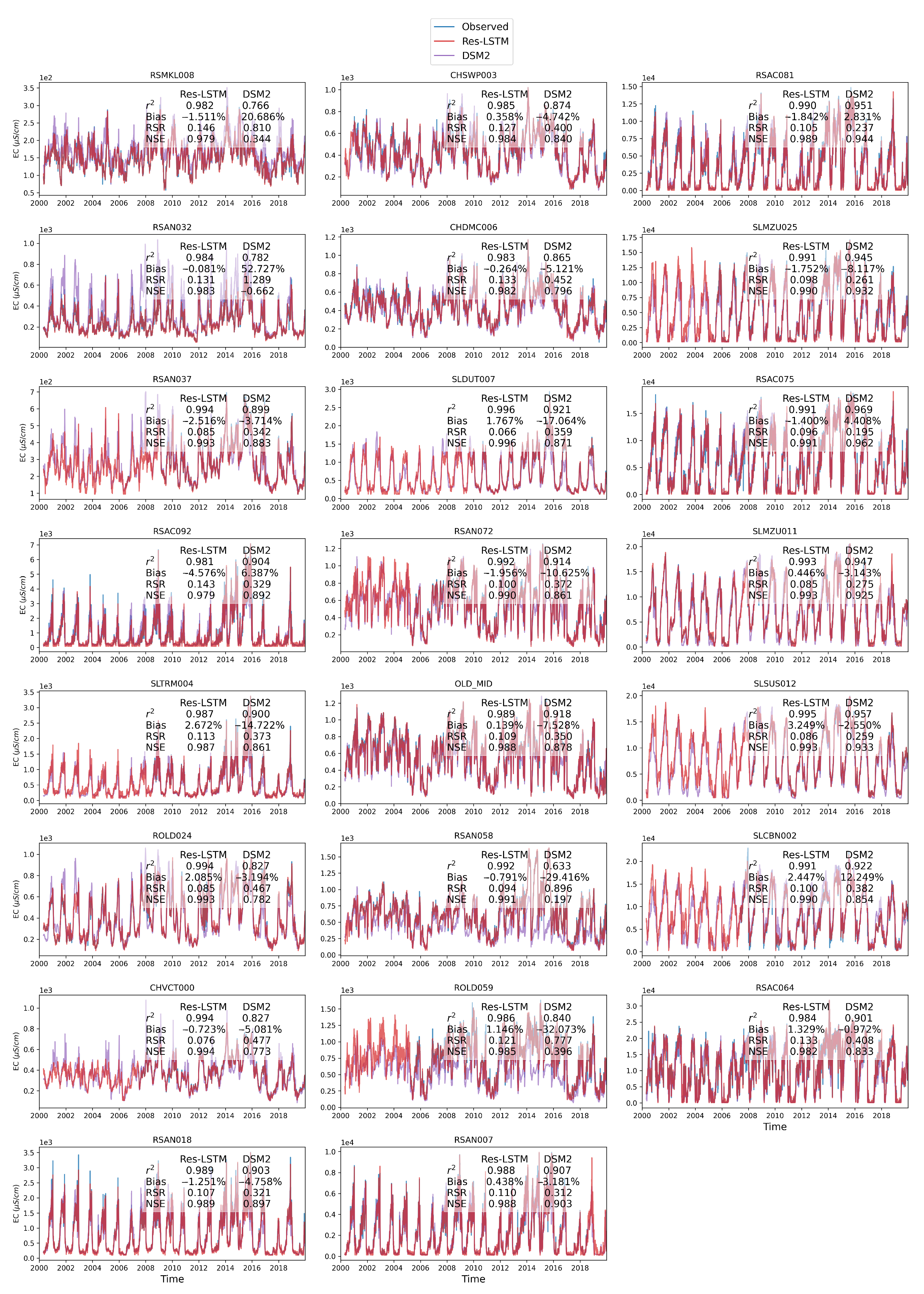
Figure A9. Time series plots of observed salinity levels versus Res-LSTM simulations and DSM2 simulations of the 23 stations. Detailed values of four evaluation metrics of Res-LSTM and DSM2 are marked for each station.
Water 14 03628 g0a9

References

  1. Alber, M. A conceptual model of estuarine freshwater inflow management. Estuaries 2002, 25, 1246–1261. [Google Scholar] [CrossRef]
  2. Rath, J.S.; Hutton, P.H.; Chen, L.; Roy, S.B. A hybrid empirical-Bayesian artificial neural network model of salinity in the San Francisco Bay-Delta estuary. Environ. Model. Softw. 2017, 93, 193–208. [Google Scholar] [CrossRef]
  3. Xu, J.; Long, W.; Wiggert, J.D.; Lanerolle, L.W.; Brown, C.W.; Murtugudde, R.; Hood, R.R. Climate forcing and salinity variability in Chesapeake Bay, USA. Estuaries Coasts 2012, 35, 237–261. [Google Scholar] [CrossRef]
  4. Tran Anh, D.; Hoang, L.P.; Bui, M.D.; Rutschmann, P. Simulating future flows and salinity intrusion using combined one-and two-dimensional hydrodynamic modelling—The case of Hau River, Vietnamese Mekong delta. Water 2018, 10, 897. [Google Scholar] [CrossRef] [Green Version]
  5. Mulamba, T.; Bacopoulos, P.; Kubatko, E.J.; Pinto, G.F. Sea-level rise impacts on longitudinal salinity for a low-gradient estuarine system. Clim. Chang. 2019, 152, 533–550. [Google Scholar] [CrossRef]
  6. MDBMC. The Salinity Audit of the Murray-Darling Basin, A 100-Year Perspective; Murray-Darling Basin Commission: Canberra, Australia, 1999. Available online: https://www.mdba.gov.au/sites/default/files/archived/mdbc-salinity-reports/2072_Salinity_audit_of_MDB_100_year_perspective.pdf (accessed on 1 July 2022).
  7. MDBMC. Basin Salinity Management 2030 (BSM2030), MDBA Publication No 21/15; Murray–Darling Basin Ministerial Council: Canberra, Australia, 2015. [Google Scholar]
  8. Myers, N.; Mittermeier, R.A.; Mittermeier, C.G.; Da Fonseca, G.A.; Kent, J. Biodiversity hotspots for conservation priorities. Nature 2000, 403, 853–858. [Google Scholar] [CrossRef]
  9. Moyle, P.B.; Brown, L.R.; Durand, J.R.; Hobbs, J.A. Delta smelt: Life history and decline of a once-abundant species in the San Francisco Estuary. San Fr. Estuary Watershed Sci. 2016, 14. [Google Scholar] [CrossRef] [Green Version]
  10. He, M.; Zhong, L.; Sandhu, P.; Zhou, Y. Emulation of a process-based salinity generator for the sacramento–san joaquin delta of california via deep learning. Water 2020, 12, 2088. [Google Scholar] [CrossRef]
  11. Healey, M.; Dettinger, M.; Norgaard, R. Perspectives on Bay–Delta Science and Policy. San Fr. Estuary Watershed Sci. 2016, 14. [Google Scholar] [CrossRef] [Green Version]
  12. CDWR. Minimum Delta Outflow Program. In Methodology for Flow and Salinity Estimates in the Sacramento-San Joaquin Delta and Suisun Marsh: 11th Annual Progress Report; CDWR: Sacramento, CA, USA, 1990. [Google Scholar]
  13. CDWR. Calibration and verification of DWRDSM. In Methodology for Flow and Salinity Estimates in the Sacramento-San Joaquin Delta and Suisun Marsh: 12th Annual Progress Report; CDWR: Sacramento, CA, USA, 1991. [Google Scholar]
  14. Denton, R.A. Accounting for Antecedent Conditions in Seawater Intrusion Modeling—Applications for the San Francisco Bay-Delta. In Hydraulic Engineering; ASCE: Reston, FL, USA, 1993; pp. 448–453. [Google Scholar]
  15. Cheng, R.T.; Casulli, V.; Gartner, J.W. Tidal, residual, intertidal mudflat (TRIM) model and its applications to San Francisco Bay, California. Estuarine, Coast. Shelf Sci. 1993, 36, 235–280. [Google Scholar] [CrossRef]
  16. DeGeorge, J.F. A Multi-Dimensional Finite Element Transport Model Utilizing a Characteristic-Galerkin Algorithm; University of California: Davis, CA, USA, 1996. [Google Scholar]
  17. Hutton, P.H.; Rath, J.S.; Chen, L.; Ungs, M.J.; Roy, S.B. Nine decades of salinity observations in the San Francisco Bay and Delta: Modeling and trend evaluations. J. Water Resour. Plan. Manag. 2016, 142, 04015069. [Google Scholar] [CrossRef] [Green Version]
  18. MacWilliams, M.; Bever, A.J.; Foresman, E. 3-D simulations of the San Francisco Estuary with subgrid bathymetry to explore long-term trends in salinity distribution and fish abundance. San Fr. Estuary Watershed Sci. 2016, 14. [Google Scholar] [CrossRef] [Green Version]
  19. MacWilliams, M.L.; Ateljevich, E.S.; Monismith, S.G.; Enright, C. An overview of multi-dimensional models of the Sacramento–San Joaquin Delta. San Fr. Estuary Watershed Sci. 2016, 14. [Google Scholar] [CrossRef] [Green Version]
  20. Chao, Y.; Farrara, J.D.; Zhang, H.; Zhang, Y.J.; Ateljevich, E.; Chai, F.; Davis, C.O.; Dugdale, R.; Wilkerson, F. Development, implementation, and validation of a modeling system for the San Francisco Bay and Estuary. Estuarine, Coast. Shelf Sci. 2017, 194, 40–56. [Google Scholar] [CrossRef]
  21. Sandhu, N.; Finch, R. Application of artificial neural networks to the Sacramento-San Joaquin Delta. In Estuarine and Coastal Modeling; ASCE: Reston, FL, USA, 1995; pp. 490–504. [Google Scholar]
  22. CDWR. Modeling Flow-Salinity Relationships in the Sacramento-San Joaquin Delta Using Artificial Neural Networks; Technical Information Record OSP-99-1; CDWR: Sacramento, CA, USA, 1999. [Google Scholar]
  23. Wilbur, R.; Munevar, A. Integration of CALSIM and Artificial Neural Networks Models for Sacramento-San Joaquin Delta Flow-Salinity Relationships. In Methodology for Flow and Salinity Estimates in the Sacramento-San Joaquin Delta and Suisun Marsh: 22nd Annual Progress Report; CDWR: Sacramento, CA, USA, 2001. [Google Scholar]
  24. Mierzwa, M. CALSIM versus DSM2 ANN and G-model Comparisons. In Methodology for Flow and Salinity Estimates in the Sacramento-San Joaquin Delta and Suisun Marsh: 23rd Annual Progress Report; CDWR: Sacramento, CA, USA, 2002. [Google Scholar]
  25. Seneviratne, S.; Wu, S. Enhanced Development of Flow-Salinity Relationships in the Delta Using Artificial Neural Networks: Incorporating Tidal Influence. In Methodology for Flow and Salinity Estimates in the Sacramento-San Joaquin Delta and Suisun Marsh: 28th Annual Progress Report; CDWR: Sacramento, CA, USA, 2007. [Google Scholar]
  26. Jayasundara, N.C.; Seneviratne, S.A.; Reyes, E.; Chung, F.I. Artificial neural network for Sacramento–San Joaquin Delta flow–salinity relationship for CalSim 3.0. J. Water Resour. Plan. Manag. 2020, 146, 04020015. [Google Scholar] [CrossRef]
  27. Qi, S.; Bai, Z.; Ding, Z.; Jayasundara, N.; He, M.; Sandhu, P.; Seneviratne, S.; Kadir, T. Enhanced Artificial Neural Networks for Salinity Estimation and Forecasting in the Sacramento-San Joaquin Delta of California. J. Water Resour. Plan. Manag. 2021, 147, 04021069. [Google Scholar] [CrossRef]
  28. Chen, L.; Roy, S.B.; Hutton, P.H. Emulation of a process-based estuarine hydrodynamic model. Hydrol. Sci. J. 2018, 63, 783–802. [Google Scholar] [CrossRef]
  29. Qi, S.; He, M.; Bai, Z.; Ding, Z.; Sandhu, P.; Zhou, Y.; Namadi, P.; Tom, B.; Hoang, R.; Anderson, J. Multi-Location Emulation of a Process-Based Salinity Model Using Machine Learning. Water 2022, 14, 2030. [Google Scholar] [CrossRef]
  30. Zounemat-Kermani, M.; Matta, E.; Cominola, A.; Xia, X.; Zhang, Q.; Liang, Q.; Hinkelmann, R. Neurocomputing in surface water hydrology and hydraulics: A review of two decades retrospective, current status and future prospects. J. Hydrol. 2020, 588, 125085. [Google Scholar] [CrossRef]
  31. Mosavi, A.; Ozturk, P.; Chau, K.W. Flood prediction using machine learning models: Literature review. Water 2018, 10, 1536. [Google Scholar] [CrossRef]
  32. Yaseen, Z.M.; Sulaiman, S.O.; Deo, R.C.; Chau, K.W. An enhanced extreme learning machine model for river flow forecasting: State-of-the-art, practical applications in water resource engineering area and future research direction. J. Hydrol. 2019, 569, 387–408. [Google Scholar] [CrossRef]
  33. Tongal, H.; Booij, M.J. Simulation and forecasting of streamflows using machine learning models coupled with base flow separation. J. Hydrol. 2018, 564, 266–282. [Google Scholar] [CrossRef]
  34. Islam, A.R.M.T.; Talukdar, S.; Mahato, S.; Kundu, S.; Eibek, K.U.; Pham, Q.B.; Kuriqi, A.; Linh, N.T.T. Flood susceptibility modelling using advanced ensemble machine learning models. Geosci. Front. 2021, 12, 101075. [Google Scholar] [CrossRef]
  35. Shahabi, H.; Shirzadi, A.; Ghaderi, K.; Omidvar, E.; Al-Ansari, N.; Clague, J.J.; Geertsema, M.; Khosravi, K.; Amini, A.; Bahrami, S.; et al. Flood detection and susceptibility mapping using sentinel-1 remote sensing data and a machine learning approach: Hybrid intelligence of bagging ensemble based on k-nearest neighbor classifier. Remote Sens. 2020, 12, 266. [Google Scholar] [CrossRef] [Green Version]
  36. Costache, R.; Hong, H.; Pham, Q.B. Comparative assessment of the flash-flood potential within small mountain catchments using bivariate statistics and their novel hybrid integration with machine learning models. Sci. Total. Environ. 2020, 711, 134514. [Google Scholar] [CrossRef]
  37. Tang, Y.; Zang, C.; Wei, Y.; Jiang, M. Data-driven modeling of groundwater level with least-square support vector machine and spatial–temporal analysis. Geotech. Geol. Eng. 2019, 37, 1661–1670. [Google Scholar] [CrossRef]
  38. El Bilali, A.; Taleb, A.; Brouziyne, Y. Groundwater quality forecasting using machine learning algorithms for irrigation purposes. Agric. Water Manag. 2021, 245, 106625. [Google Scholar] [CrossRef]
  39. Yin, J.; Medellín-Azuara, J.; Escriva-Bou, A.; Liu, Z. Bayesian machine learning ensemble approach to quantify model uncertainty in predicting groundwater storage change. Sci. Total. Environ. 2021, 769, 144715. [Google Scholar] [CrossRef]
  40. Kumar, D.; Pandey, A.; Sharma, N.; Flügel, W.A. Daily suspended sediment simulation using machine learning approach. Catena 2016, 138, 77–90. [Google Scholar] [CrossRef]
  41. Choubin, B.; Darabi, H.; Rahmati, O.; Sajedi-Hosseini, F.; Kløve, B. River suspended sediment modelling using the CART model: A comparative study of machine learning techniques. Sci. Total. Environ. 2018, 615, 272–281. [Google Scholar] [CrossRef]
  42. Melesse, A.M.; Khosravi, K.; Tiefenbacher, J.P.; Heddam, S.; Kim, S.; Mosavi, A.; Pham, B.T. River water salinity prediction using hybrid machine learning models. Water 2020, 12, 2951. [Google Scholar] [CrossRef]
  43. Nauman, T.W.; Ely, C.P.; Miller, M.P.; Duniway, M.C. Salinity yield modeling of the Upper Colorado River Basin using 30-m resolution soil maps and random forests. Water Resour. Res. 2019, 55, 4954–4973. [Google Scholar] [CrossRef]
  44. Derot, J.; Yajima, H.; Jacquet, S. Advances in forecasting harmful algal blooms using machine learning models: A case study with Planktothrix rubescens in Lake Geneva. Harmful Algae 2020, 99, 101906. [Google Scholar] [CrossRef]
  45. Alizadeh, M.J.; Kavianpour, M.R.; Danesh, M.; Adolf, J.; Shamshirband, S.; Chau, K.W. Effect of river flow on the quality of estuarine and coastal waters using machine learning models. Eng. Appl. Comput. Fluid Mech. 2018, 12, 810–823. [Google Scholar] [CrossRef] [Green Version]
  46. Shamshirband, S.; Jafari Nodoushan, E.; Adolf, J.E.; Abdul Manaf, A.; Mosavi, A.; Chau, K.w. Ensemble models with uncertainty analysis for multi-day ahead forecasting of chlorophyll a concentration in coastal waters. Eng. Appl. Comput. Fluid Mech. 2019, 13, 91–101. [Google Scholar] [CrossRef] [Green Version]
  47. Jiang, Y.; Zhang, T.; Gou, Y.; He, L.; Bai, H.; Hu, C. High-resolution temperature and salinity model analysis using support vector regression. J. Ambient. Intell. Humaniz. Comput. 2018, 1–9. [Google Scholar] [CrossRef]
  48. Thai-Nghe, N.; Thanh-Hai, N.; Chi Ngon, N. Deep learning approach for forecasting water quality in IoT systems. Int. J. Adv. Comput. Sci. Appl. 2020, 11, 686–693. [Google Scholar] [CrossRef]
  49. Granata, F.; Papirio, S.; Esposito, G.; Gargano, R.; De Marinis, G. Machine learning algorithms for the forecasting of wastewater quality indicators. Water 2017, 9, 105. [Google Scholar] [CrossRef] [Green Version]
  50. Barzegar, R.; Asghari Moghaddam, A.; Adamowski, J.; Ozga-Zielinski, B. Multi-step water quality forecasting using a boosting ensemble multi-wavelet extreme learning machine model. Stoch. Environ. Res. Risk Assess. 2018, 32, 799–813. [Google Scholar] [CrossRef]
  51. Ahmed, A.N.; Othman, F.B.; Afan, H.A.; Ibrahim, R.K.; Fai, C.M.; Hossain, M.S.; Ehteram, M.; Elshafie, A. Machine learning methods for better water quality prediction. J. Hydrol. 2019, 578, 124084. [Google Scholar] [CrossRef]
  52. Ghalambor, C.K.; Gross, E.S.; Grosholtz, E.D.; Jeffries, K.M.; Largier, J.K.; McCormick, S.D.; Sommer, T.; Velotta, J.; Whitehead, A. Ecological Effects of Climate-Driven Salinity Variation in the San Francisco Estuary: Can We Anticipate and Manage the Coming Changes? San Fr. Estuary Watershed Sci. 2021, 19. [Google Scholar] [CrossRef]
  53. Lund, J.R. California’s agricultural and urban water supply reliability and the Sacramento–San Joaquin Delta. San Fr. Estuary Watershed Sci. 2016, 14. [Google Scholar] [CrossRef] [Green Version]
  54. Namadi, P.; He, M.; Sandhu, P. Salinity-constituent conversion in South Sacramento-San Joaquin Delta of California via machine learning. Earth Sci. Informatics 2022, 15, 1–16. [Google Scholar] [CrossRef]
  55. He, K.; Zhang, X.; Ren, S.; Sun, J. Deep residual learning for image recognition. In Proceedings of the IEEE Conference on Computer Vision and Pattern Recognition, Las Vegas, NV, USA, 27–30 June 2016; pp. 770–778. [Google Scholar]
  56. Kingma, D.P.; Ba, J. Adam: A method for stochastic optimization. arXiv 2014, arXiv:1412.6980. [Google Scholar]
  57. Panda, S.S.; Amatya, D.M.; Muwamba, A.; Chescheir, G. Estimation of evapotranspiration and its parameters for pine, switchgrass, and intercropping with remotely-sensed images based geospatial modeling. Environ. Model. Softw. 2019, 121, 104487. [Google Scholar] [CrossRef]
  58. Dietterich, T. Overfitting and undercomputing in machine learning. ACM Comput. Surv. (CSUR) 1995, 27, 326–327. [Google Scholar] [CrossRef]
  59. Ying, X. An overview of overfitting and its solutions. In Journal of Physics; Conference Series; IOP Publishing: Bristol, UK, 2019; Volume 1168, p. 022022. [Google Scholar]
  60. Adadi, A.; Berrada, M. Peeking inside the black-box: A survey on explainable artificial intelligence (XAI). IEEE Access 2018, 6, 52138–52160. [Google Scholar] [CrossRef]
  61. Ancona, M.; Ceolini, E.; Öztireli, C.; Gross, M. Towards better understanding of gradient-based attribution methods for deep neural networks. arXiv 2017, arXiv:1711.06104. [Google Scholar]
  62. Shrikumar, A.; Greenside, P.; Kundaje, A. Learning important features through propagating activation differences. In Proceedings of the International Conference on Machine Learning, PMLR, Sydney, Australia, 6–11 August 2017; pp. 3145–3153. [Google Scholar]
  63. Dettinger, M.; Anderson, J.; Anderson, M.; Brown, L.R.; Cayan, D.; Maurer, E. Climate change and the Delta. San Fr. Estuary Watershed Sci. 2016, 14. [Google Scholar] [CrossRef] [Green Version]
  64. Wilson, T.S.; Sleeter, B.M.; Cameron, D.R. Future land-use related water demand in California. Environ. Res. Lett. 2016, 11, 054018. [Google Scholar] [CrossRef]
  65. Kimmerer, W.; Wilkerson, F.; Downing, B.; Dugdale, R.; Gross, E.S.; Kayfetz, K.; Khanna, S.; Parker, A.E.; Thompson, J. Effects of drought and the emergency drought barrier on the ecosystem of the California Delta. San Fr. Estuary Watershed Sci. 2019, 17. [Google Scholar] [CrossRef] [Green Version]
  66. Raissi, M.; Perdikaris, P.; Karniadakis, G.E. Physics-informed neural networks: A deep learning framework for solving forward and inverse problems involving nonlinear partial differential equations. J. Comput. Phys. 2019, 378, 686–707. [Google Scholar] [CrossRef]
  67. Lu, L.; Meng, X.; Mao, Z.; Karniadakis, G.E. DeepXDE: A deep learning library for solving differential equations. Siam Rev. 2021, 63, 208–228. [Google Scholar] [CrossRef]
  68. Gay, P.S.; O’Donnell, J. A simple advection-dispersion model for the salt distribution in linearly tapered estuaries. J. Geophys. Res. Ocean. 2007, 112. [Google Scholar] [CrossRef]
Figure 1. Schematic showing the Sacramento–San Joaquin Delta (Delta), the 23 study locations, and the DSM2 model domain.
Water 14 03628 g001
Figure 2. Boxplot of salinity observations (represented by electrical conductivity) at study locations, sorted by their medians. Numbers next to each station’s box represent the ratios of available observations in the dataset during the 20-year study period. Each box represents the interquartile range from the 25th to the 75th percentiles. The line inside each box represents the median value. The open circles represent outliers.
Water 14 03628 g002
Figure 3. Diagram of the proposed Res-LSTM network. The number in the input layer denotes input shape and those in the subsequent layers represent the numbers of units / neurons of those layers.
Water 14 03628 g003
Figure 4. Diagram of the proposed Res-GRU network. The number in the input layer denotes input shape and those in the subsequent layers represent the numbers of units / neurons of those layers.
Water 14 03628 g004
Figure 5. Comparison of six models on observed data at daily time step.
Water 14 03628 g005
Figure 6. Exceedance probability plot and time series plot of Res-LSTM simulated versus observed salinity at daily time step.
Water 14 03628 g006
Figure 7. Heatmap showing Res-LSTM performance at different salinity ranges on the daily time step: low–middle range (lowest 75%), high range (75 to 95 percentile), and extreme high range (highest 5%) at the study locations.
Water 14 03628 g007
Figure 8. Salinity forecasting performance of Res-LSTM.
Water 14 03628 g008
Figure 9. Salinity forecasting performance of Res-GRU.
Water 14 03628 g009
Figure 10. Comparison of six models on observed data at hourly time step with daily inputs.
Water 14 03628 g010
Figure 11. Exceedance probability plot and time series plot of Res-LSTM simulated versus observed salinity at daily time step with daily inputs.
Water 14 03628 g011
Figure 12. Heatmap showing Res-LSTM performance at different salinity ranges on the hourly time step: low–middle range (lowest 75%), high range (75 to 95 percentile), and extreme high range (highest 5%) at the study locations.
Water 14 03628 g012
Figure 13. Model performance versus total numbers of parameters of the proposed models and their variants with varying structural complexities.
Water 14 03628 g013
Figure 14. Time series plots of observed salinity levels versus Res-LSTM simulations and DSM2 simulations of six key stations. Detailed values of four evaluation metrics of Res-LSTM and DSM2 are marked for each station.
Water 14 03628 g014
Table 1. Input features to proposed ML models.
IndexInput Feature NameDefinition
1Northern FlowSum of Sacramento, Yolo Bypass, Mokelumne River, Cosumnes River, and Calaveras River flows.
2San Joaquin River FlowSan Joaquin River at Vernalis Flow.
3PumpingSum of pumping from Banks Pumping Plant, Jones Pumping Plant, and Contra Costa Water District at Rock Slough, Old River, and Victoria Canal.
4Delta Cross-Channel Gate OperationDelta Cross-Channel Gate Openings.
5Consumptive UseNet Delta Consumptive use estimated by Delta Channel Depletion (DCD) and Suisun Marsh Channel Depletion (SMCD) models.
6Martinez Tidal EnergyTidal energy at Martinez, calculated as the daily maximum–the daily minimum astronomical tide at Martinez.
7San Joaquin River ECElectrical conductivity measured at San Joaquin River at Vernalis.
8Sacramento River ECElectrical conductivity measured at Sacramento River at Greens Landing.
Table 2. Number of parameters of the six ML models.
ArchitectureMLPResNetLSTMGRURes-LSTMRes-GRU
Number of parameters36, 271357,799227,263201,687111,300100,812
Table 3. Study metrics.
NameDefinitionFormula
MSEMean Squared ErrorMSE = t = t l + 1 T ( S O b s e r v e d t S A N N t ) 2
r 2 Squared Correlation Coefficient r 2 = ( t = t l + 1 T | ( S O b s e r v e d t S O b s e r v e d ¯ ) × ( S A N N t S A N N ¯ ) | T × σ O b s e r v e d × σ A N N ) 2
BiasPercent BiasBias = t = t l + 1 T ( S A N N t S O b s e r v e d t ) t = t l + 1 T S O b s e r v e d t × 100 %
RSRRMSE-observations standard deviation ratioRSR = t = t l + 1 T ( S O b s e r v e d t S A N N t ) 2 t = t l + 1 T ( S O b s e r v e d t S O b s e r v e d ¯ ) 2
NSENash-Sutcliffe Efficiency coefficientNSE = 1 t = t l + 1 T ( S O b s e r v e d t S A N N t ) 2 t = t l + 1 T ( S O b s e r v e d t S O b s e r v e d ¯ ) 2
Publisher’s Note: MDPI stays neutral with regard to jurisdictional claims in published maps and institutional affiliations.