
An Analytical Solution to Predict the Distribution of Streamwise Flow Velocity in an Ecological River with Submerged Vegetation
Abstract
1. Introduction
2. Theoretical Analysis
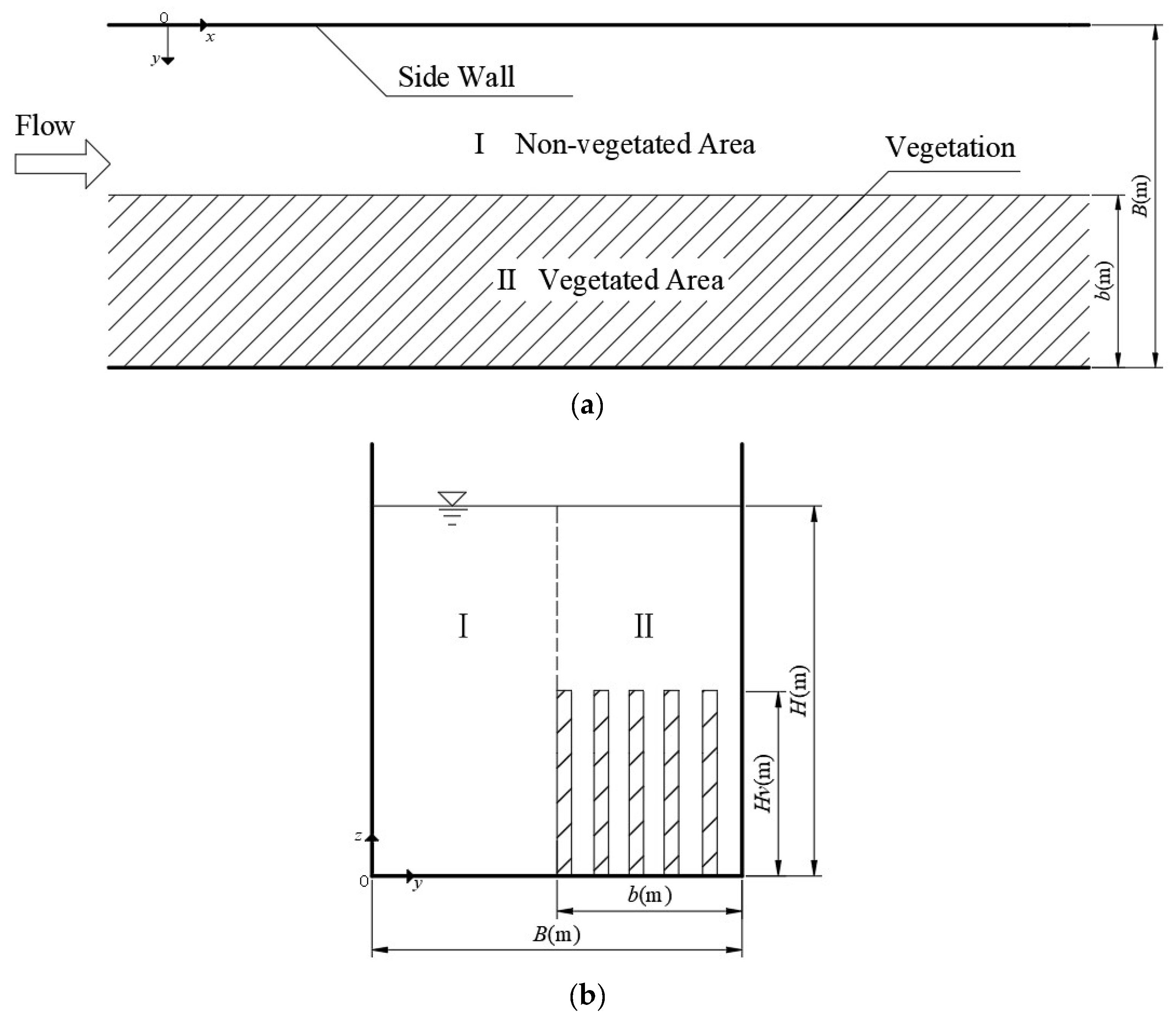
- For the non-vegetated area, i.e., the area I in Figure 1b, the solutions of Equation (20) for the non-vegetated area and vegetated area are different. This is because, for the non-vegetated area, the drag force coefficient is 0 in Equation (20). Ignoring the vegetation resistance term “”, Ud is expressed as follows:
- 2.
- For the vegetated area, i.e., area II in Figure 1b, Ud is expressed as follows:
3. Boundary Conditions
- (1)
- On the side wall, the no-slip boundary condition is present, and for the velocity near the side wall, i.e., when y = 0 and y = B, Ud = 0 (two boundary conditions).
- (2)
- The velocity continuity condition exists at the junction between the non-vegetated area and the vegetated area, i.e., when y = B, Ud(i) = Ud(i + 1).
- (3)
- The stress continuity condition is present when the water flow is uniform at the junction between the non-vegetated and vegetated areas. Thus, the flow depth transition is not abrupt at the junction between the areas. The stress continuity condition can be expressed as follows:
4. Parameter Determination
4.1. Transverse Eddy Viscosity Coefficient ξ
4.2. Darcy–Weisbach Friction Coefficient f
4.3. Porosity α
4.4. The Drag Force Coefficient Cd
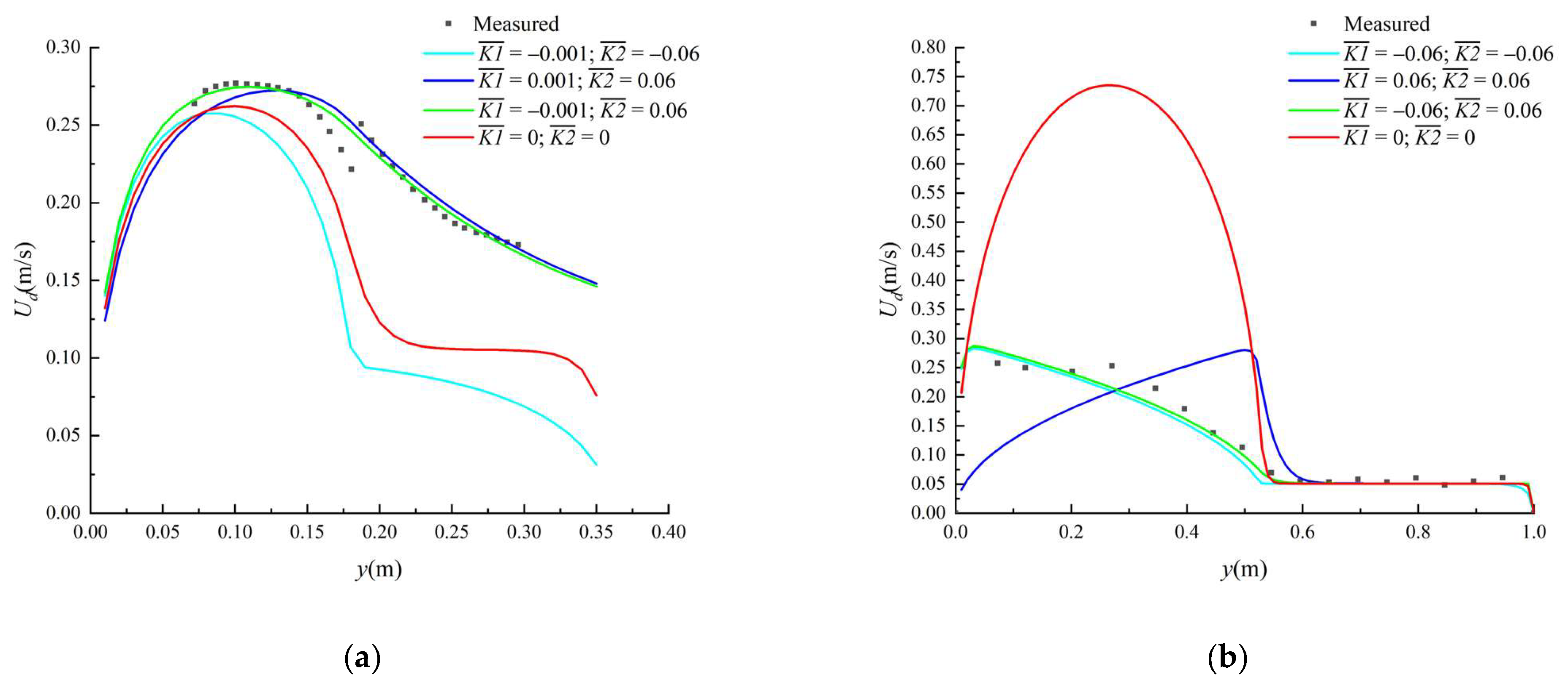
4.5. Secondary Flow Coefficients and
5. Experimental Data
5.1. Experimental Data Obtained by Naot et al. [32]
5.2. Experimental Data Obtained by Shi and Huai [33]
6. Comparison of Theoretical and Experimental Data
7. Discussion
8. Conclusions
Author Contributions
Funding
Institutional Review Board Statement
Informed Consent Statement
Conflicts of Interest
Notation
| Av | projected vegetated area per unit volume in the direction of downstream flow |
| B | width of the flume |
| b | width of the vegetation layer |
| Cd | drag force coefficient for vegetation |
| D | vegetation stem diameter |
| Dr | relative depth ratio |
| Fv | drag force |
| f | Darcy–Weisbach friction coefficient |
| g | gravitational acceleration |
| H | flow depth |
| Hv | height of vegetation |
| secondary flow coefficient | |
| m | number of vegetation per unit of area |
| N | non-dimensional vegetation density |
| S0 | channel bed slope |
| Uv | depth-averaged streamwise velocity along the vegetation height |
| Ud | water depth-averaged streamwise velocity |
| ρ | flow density |
| α | porosity |
| β | shape factor of the vegetation |
| ξ | transverse eddy viscosity coefficient |
| φ | Uv/Ud |
| average value of absolute error | |
| average value of relative error |
References
- Harvey, J.W.; Noe, G.B.; Larsen, L.G.; Nowacki, D.J.; Mcphillips, L.E. Field flume reveals aquatic vegetation’s role in sediment and particulate phosphorus transport in a shallow aquatic ecosystem. Geomorphology 2011, 126, 297–313. [Google Scholar] [CrossRef]
- Cullen-Unsworth, L.; Unsworth, R. Seagrass meadows, ecosystem services, and sustainability. Environ. Sci. Policy Sustain. Dev. 2013, 55, 14–28. [Google Scholar] [CrossRef]
- Scholle, M.; Aksel, N. An exact solution of visco-capillary flow in an inclined channel. Z. Angew. Math. Phys. 2001, 52, 749–769. [Google Scholar] [CrossRef]
- White, B.L.; Nepf, H.M. A vortex-based model of velocity and shear stress in a partially vegetated shallow channel. Water Resour. Res. 2008, 44, W01412. [Google Scholar] [CrossRef]
- Terrier, B. Flow Characteristics in Straight Compound Channels with Vegetation along the Main Channel. Ph.D. Thesis, Loughborough University, Loughborough, UK, 2010. [Google Scholar]
- Shiono, K.; Knight, D.W. Turbulent open-channel flows with variable depth across the channel. J. Fluid Mech. 1991, 222, 617–646. [Google Scholar] [CrossRef]
- Liu, C.; Shan, Y. Impact of an emergent model vegetation patch on flow adjustment and velocity. In Proceedings of the Institution of Civil Engineers—Water Management; Thomas Telford Ltd.: London, UK, 2022; Volume 175, pp. 55–66. [Google Scholar] [CrossRef]
- Liu, C.; Shan, Y.; Sun, W.; Yan, C.; Yang, K. An open channel with an emergent vegetation patch: Predicting the longitudinal profiles of velocities based on exponential decay. J. Hydrol. 2020, 582, 124429. [Google Scholar] [CrossRef]
- Huai, W.; Gao, M.; Zeng, Y.; Li, D. Two-dimensional analytical solution for compound channel flows with vegetated floodplains. Appl. Math. Mech. 2009, 30, 1049–1056. [Google Scholar] [CrossRef]
- Fu, X.; Wang, F.; Liu, M.; Huai, W. Transverse distribution of the streamwise velocity for the open-channel flow with floating vegetated islands. Environ. Sci. Pollut. Res. Int. 2021, 28, 51265–51277. [Google Scholar] [CrossRef]
- Devi, K.; Khatua, K.K. Prediction of depth averaged velocity and boundary shear distribution of a compound channel based on the mixing layer theory. Flow Meas. Instrum. 2016, 50, 147–157. [Google Scholar] [CrossRef]
- Sun, Z.; Zheng, J.; Zhu, L.; Chong, L.; Liu, J.; Luo, J. Influence of submerged vegetation on flow structure and sediment deposition. J. Zhejiang Univ. (Eng. Sci.) 2021, 55, 71–80. [Google Scholar] [CrossRef]
- Liu, C.; Luo, X.; Liu, X.; Yang, K. Modeling depth-averaged velocity and bed shear stress in compound channels with emergent and submerged vegetation. Adv. Water Resour. 2013, 60, 148–159. [Google Scholar] [CrossRef]
- Yang, K.; Cao, S.; Knight, D.W. Flow patterns in compound channels with vegetated floodplains. J. Hydraul. Eng. 2007, 133, 148–159. [Google Scholar] [CrossRef]
- Kowalski, J.; Torrilhon, M. Moment approximations and model cascades for shallow flow. Commun. Comput. Phys. 2019, 25, 669–702. [Google Scholar] [CrossRef]
- Koellermeier, J.; Rominger, M. Analysis and numerical simulation of hyperbolic shallow water moment equations. Commun. Comput. Phys. 2020, 28, 1038–1084. [Google Scholar] [CrossRef]
- Wang, W.; Liu, Z.; Chen, Y.; Zhu, D. Vertical profile of horizontal velocity in the flow with submerged vegetation. J. Sichuan Univ. (Eng. Sci. Ed.) 2012, 44, 253–257. [Google Scholar] [CrossRef]
- Huai, W.; Zeng, Y.; Xu, Z.; Yang, Z. Three-layer model for vertical velocity distribution in open channel flow with submerged rigid vegetation. Adv. Water Resour. 2009, 32, 487–492. [Google Scholar] [CrossRef]
- Castro, M.J.; Macias, J.; Pares, C. A q-scheme for a class of systems of coupled conservation laws with source term. application to a two-layer 1-d shallow water system. ESAIM: Math. Model. Numer. Anal. 2001, 35, 107–127. [Google Scholar] [CrossRef]
- Ghisalberti, M.; Nepf, H. Shallow flows over a permeable medium: The hydrodynamics of submerged aquatic canopies. Transp. Porous Media 2009, 78, 309. [Google Scholar] [CrossRef]
- Wang, W.; Huai, W.; Li, S.; Wang, P.; Wang, Y.; Zhang, J. Analytical solutions of velocity profile in flow through submerged vegetation with variable frontal width. J. Hydrol. 2019, 578, 124088. [Google Scholar] [CrossRef]
- Sukhodolov, A.N.; Sukhodolova, T.A. Case study: Effect of submerged aquatic plants on turbulence structure in a Lowland River. J. Hydraul. Eng. 2010, 136, 434–446. [Google Scholar] [CrossRef]
- Liu, H.; Zhang, J.; Hu, T. Analysis of local flow field characteristics of non-submerged cylinder group. Shanghai Jiao Tong Univ. 2016, 31, 161–170. [Google Scholar]
- Yang, Y.; Ma, Y.; Zhan, Z.; Fang, S.L.; Zhang, M. Fine numerical simulation of three-dimensional hydrodynamics in vegetation area under submerged and floating vegetation. In Proceedings of the 31st National Symposium on Hydrodynamics; Ocean Press: Lancing, UK, 2020; Volume II. [Google Scholar]
- Stone, B.M.; Shen, H. Hydraulic resistance of flow in channels with cylindrical roughness. J. Hydraul. Eng. 2002, 128, 500–506. [Google Scholar] [CrossRef]
- Cheng, N.S. Representative roughness height of submerged vegetation. Water Resour. Res. 2011, 47, W08517. [Google Scholar] [CrossRef]
- Huthoff, F.; Augustijn, D.C.M.; Hulscher, S.J.M.H. Analytical solution of the depth-averaged flow velocity in case of submerged rigid cylindrical vegetation. Water Resour. Res. 2007, 43. [Google Scholar] [CrossRef]
- Abril, J.B.; Knight, D.W. Stage-discharge prediction for rivers in flood applying a depth-averaged model. J. Hydraul. Res. 2004, 42, 616–629. [Google Scholar] [CrossRef]
- Pasche, E.; Rouvé, G. Overbank flow with vegetatively roughened flood plains. J. Hydraul. Eng. 1985, 111, 1262–1278. [Google Scholar] [CrossRef]
- Rameshwaran, P.; Shiono, K. Quasi two-dimensional model for straight overbank flows through emergent. J. Hydraul. Res. 2007, 45, 302–315. [Google Scholar] [CrossRef]
- Ackers, P. Hydraulic design of straight compound channels. Detail. Dev. Des. Method 1991, 2, 1–139. [Google Scholar]
- Naot, D. Hydrodynamic behavior of partly vegetated open channels. J. Hydraul. Eng. 1996, 122, 625–633. [Google Scholar] [CrossRef]
- Shi, H.; Huai, W. Two-Dimensional Analytical Solution for a Compound Open Channel Flow with Submerged Vegetation. Sciencepaper Online. 2016. Available online: http://www.paper.edu.cn/releasepaper/content/201612-315 (accessed on 12 September 2022).
- Tanino, Y.; Nepf, H.M. Laboratory investigation of mean drag in a random array of rigid, emergent cylinders. J. Hydraul. Eng. 2008, 134, 34–41. [Google Scholar] [CrossRef]
- James, C.S.; Birkhead, A.L.; Jordanova, A.A.; O’Sullivan, J.J. Flow resistance of emergent vegetation. J. Hydraul. Res. 2004, 42, 390–398. [Google Scholar] [CrossRef]
- Wang, C.; Zhang, H. Hydrodynamic and mixing characteristics of a river confluence with floodplain. J. Hohai Univ. (Nat. Sci.) 2022, 1–13. Available online: http://kns.cnki.net/kcms/detail/32.1117.TV.20220628.1720.008.html (accessed on 12 September 2022).
- Zhang, M. Study on Flow Characteristics of Compound Channel with Vegetation Floodplain. Ph.D. Thesis, Tsinghua University, Beijing, China, 2011. [Google Scholar]


| Sources | Cases | H (m) | Hv (m) | D (m) | m (m−2) | β | Re | ||
|---|---|---|---|---|---|---|---|---|---|
| Naot et al. [32] | 1 | 0.06 | 0.03 | 0.0036 | 278 | 0.51 | −0.0009 | 0.15 | 9000 |
| 2 | 0.06 | 0.03 | 0.0036 | 1111 | 0.43 | −0.001 | 0.06 | 9000 | |
| 3 | 0.06 | 0.03 | 0.0036 | 4444 | 0.26 | −0.001 | 0.06 | 9000 | |
| Shi and Huai [33] | 4 | 0.31 | 0.25 | 0.008 | 400 | 1 | −0.06 | 0.06 | 8550 |
| Sources | The Average Value of Error | Cases | |||
|---|---|---|---|---|---|
| Case 1 | Case 2 | Case 3 | Case 4 | ||
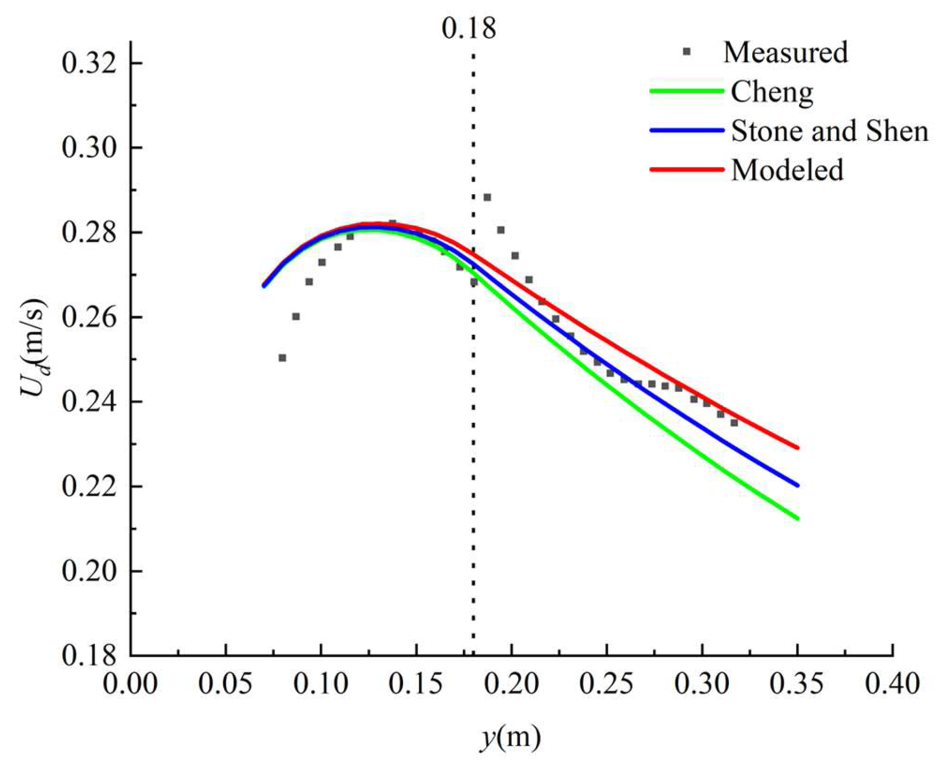
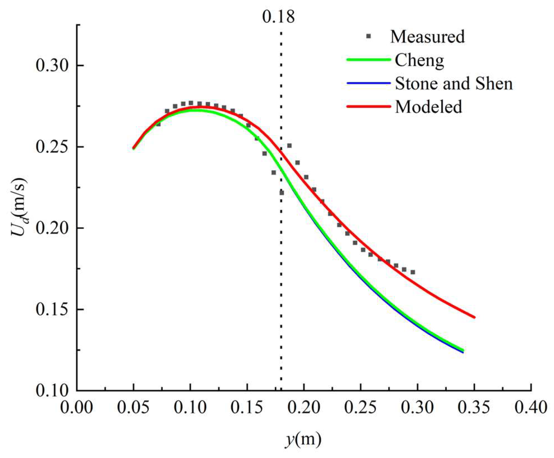
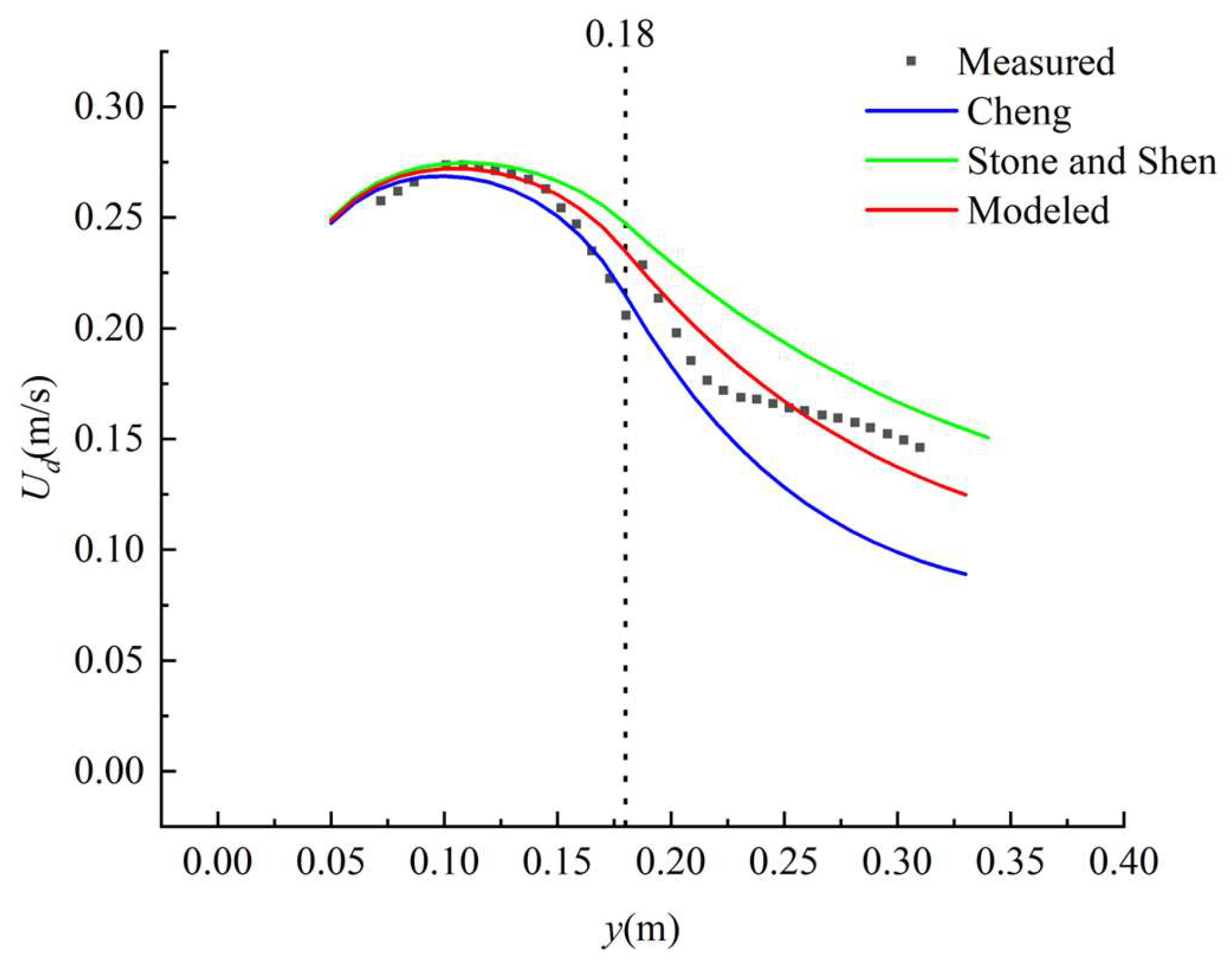
| Cheng [26] | 0.0072 | 0.0125 | 0.0191 | 0.0045 | |
| (%) | 2.8 | 6.15 | 10.3 | 5.47 | |
| Stone and Shen [25] | 0.0047 | 0.0131 | 0.02 | 0.0059 | |
| (%) | 1.81 | 6.47 | 11.7 | 8.04 | |
| Present Model | 0.0048 | 0.0041 | 0.0080 | 0.004 | |
| (%) | 1.85 | 1.84 | 4.34 | 4.77 | |
| Sources | ||||
|---|---|---|---|---|
| Present Model | ||||
| Case 2 | = −0.001 = 0.06 | = 0.001 = 0.06 | = −0.001 = −0.06 | = 0 |
| Case 4 | = −0.06 = 0.06 | = 0.06 = 0.06 | = −0.06 = −0.06 | = 0 |
Publisher’s Note: MDPI stays neutral with regard to jurisdictional claims in published maps and institutional affiliations. |
© 2022 by the authors. Licensee MDPI, Basel, Switzerland. This article is an open access article distributed under the terms and conditions of the Creative Commons Attribution (CC BY) license (https://creativecommons.org/licenses/by/4.0/).
Share and Cite
Zhang, J.; Mi, Z.; Wang, W.; Li, Z.; Wang, H.; Wang, Q.; Zhang, X.; Du, X. An Analytical Solution to Predict the Distribution of Streamwise Flow Velocity in an Ecological River with Submerged Vegetation. Water 2022, 14, 3562. https://doi.org/10.3390/w14213562
Zhang J, Mi Z, Wang W, Li Z, Wang H, Wang Q, Zhang X, Du X. An Analytical Solution to Predict the Distribution of Streamwise Flow Velocity in an Ecological River with Submerged Vegetation. Water. 2022; 14(21):3562. https://doi.org/10.3390/w14213562
Chicago/Turabian StyleZhang, Jiao, Zhangyi Mi, Wen Wang, Zhanbin Li, Huilin Wang, Qingjing Wang, Xunle Zhang, and Xinchun Du. 2022. "An Analytical Solution to Predict the Distribution of Streamwise Flow Velocity in an Ecological River with Submerged Vegetation" Water 14, no. 21: 3562. https://doi.org/10.3390/w14213562
APA StyleZhang, J., Mi, Z., Wang, W., Li, Z., Wang, H., Wang, Q., Zhang, X., & Du, X. (2022). An Analytical Solution to Predict the Distribution of Streamwise Flow Velocity in an Ecological River with Submerged Vegetation. Water, 14(21), 3562. https://doi.org/10.3390/w14213562