Calibration and Evaluation of Empirical Methods to Estimate Reference Crop Evapotranspiration in West Texas

Abstract

Evapotranspiration is an essential component of the hydrologic cycle, and its accurate quantification is crucial for managing crop water requirements and the operation of irrigation systems. Evapotranspiration data is key to hydrological and water management research investigations, including studying the impact of various climatic factors on crop water requirements. It has been estimated as the product of the reference crop evapotranspiration and crop coefficient. Daily reference crop evapotranspiration (ET_o) can be determined by several methods and equations. The Food and Agriculture Organization Penman-Monteith equation requires complete weather data, whereas empirical equations such as Hargreaves and Samani, Valiantzas, Priestley-Taylor, Makkink, and Stephens-Stewart require limited weather data. This work evaluated different empirical equations for West Texas using the standard FAO Penman-Monteith method and calibrated their parameters to improve ET_o estimation. Detailed meteorological data from West Texas Mesonet and high resolution (800 m) Parameter-elevation Regressions on Independent Slopes Model (PRISM) datasets from 2007 to 2016 were used. Daily ET_o calculated using the standard FAO Penman-Monteith equation was compared to ET_o estimated based on different empirical methods. The results show that all original empirical equations underestimated ET_o. Calibration improved the performance of tested equations; however, there seems to be underestimation of ET_o in the 8–16 mm range. Overall, the monthly Hargreaves and Samani equation with either original or calibrated values of its parameters outperformed all tested models. This equation seems to be a reasonable estimator, especially under limited weather data conditions.

1. Introduction

According to Texas Water Development Board [1], Texas’ population is expected to increase by more than 73 percent from 29.7 to 51.5 million between 2020 and 2070; however, water demands are projected to increase less significantly, by approximately 9% from 21.8 billion to 23.7 billion m³ per year during the same period. Currently, irrigated agriculture is the largest user of freshwater in Texas; it uses 53% of the freshwater resources in the state [1]. In 2017, Texas ranked fourth in the United States in agricultural irrigated acreages and irrigation water use [2]. However, irrigation demand is expected to decrease, from 11.65 in 2020 to 9.37 billion m³ per year in 2070, due to more efficient irrigation systems, reduced groundwater supplies, and the transfer of water rights from agricultural to municipal uses [1]. Moreover, the projected doubling of population, i.e., increased competition for water, presents more challenges for sustainable irrigated agriculture [3]. Under these circumstances, the availability of irrigation water is more critical with the increasing food demands of the future population [3].

The availability of irrigation water can be increased through water-saving by adopting various improved water management techniques. Such practices raise the productivity of water use and help optimize the use of the limited available water. One of the essential steps in this process is improving irrigation scheduling [4,5,6,7], which aims to apply an adequate amount of irrigation water without causing crop water stress and/or excess water losses while ensuring optimum crop yields. Irrigation scheduling is the process through which we determine when and for how long to irrigate a particular crop to meet its water requirements [6,8]; thus, accurate knowledge of Crop Evapotranspiration (ETc) is key to the success of any irrigation scheduling program. Measuring crop evapotranspiration at high spatio-temporal resolutions is costly in time and effort; however, estimating it based on Reference Crop Evapotranspiration (ET_o) [9] is possible based on readily available limited weather data. Multiple weather networks have been established in different parts of Texas; however, despite these efforts, there is still a lack of dedicated funding to ensure uninterrupted weather monitoring across a large state, limiting these networks’ availability and sustainability [3].

Several approaches have been developed to estimate ET_o with limited weather data, including the FAO-Penman-Monteith [9], Hargreaves-Samani [10], Valiantzas [11], Priestley-Taylor [12], Stephens-Stewart [13], Makkink [14], and Monthly Hargreaves-Samani [15]. ET_o estimation by PM model does not require local calibration and is considered the best method in different climatic conditions. The Food and Agriculture Organization of the United Nations (FAO) has recommended it as the standard method to calculate ET_o [9]. The FAO Penman-Monteith (FAO-PM) model has been used in various studies [16,17,18,19]; however, it requires complete weather data, including air temperature, relative humidity, wind speed, and solar radiation, most of which are not available in all regions. Radiation- and temperature-based ET_o models are widely used, especially when complete weather data is not available. However, studies show that the performance of such methods is remarkably affected outside regions in which they were initially developed [20,21,22,23]. Thus, to improve their accuracy and reliability of prediction, site-specific calibration is required.

This study aims to assess the performance of six radiation- and temperature-based models compare with the Food and Agriculture Organization of the United Nations (FAO) Penman-Monteith model with and without calibration for West Texas conditions.

The rest of this paper is organized as follows. Section 2 and Section 3 have detailed information about the study area, data used, and research approach and methods used. However, Section 4 covers the results and discussions. Finally, Section 5 summarizes the conclusions of the study.

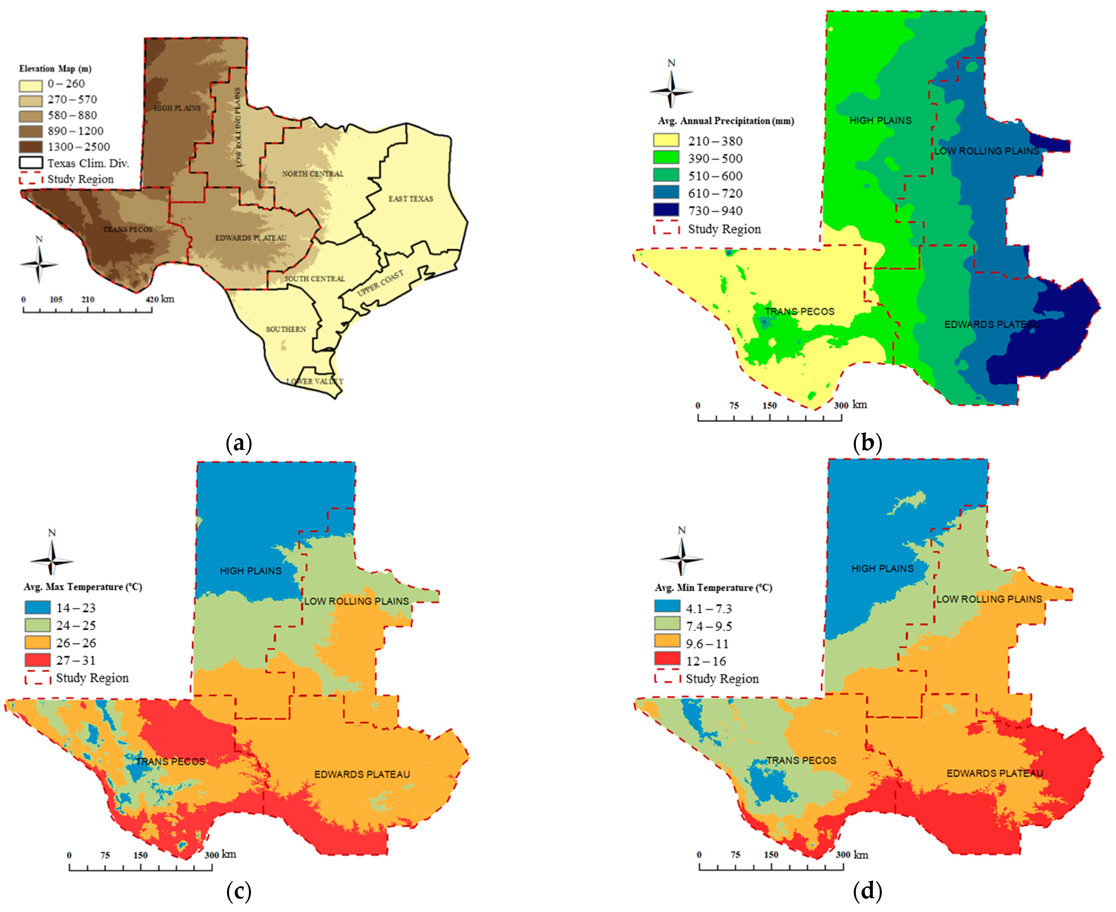
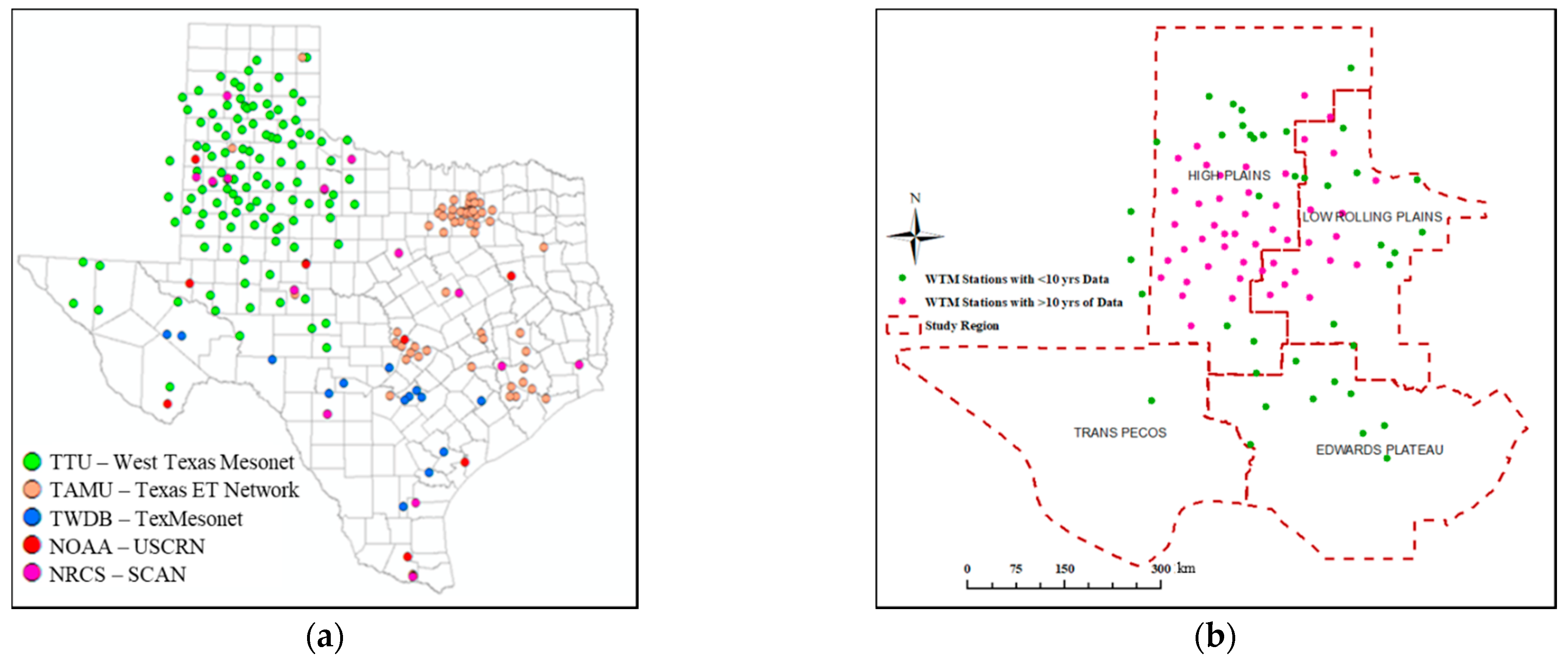
2. Study Area and Data Used

The climate of Texas is spatially diverse; the National Climate Data Center (NCDC) splits it into ten climate regions based on temperature, humidity, precipitation, and seasonal weather variability characteristics (Figure 1a). The state’s geographic location in the continent and its interactions with large circulation systems, distributions of atmospheric pressure, and jet streams have resulted in the variability of Texas’ climate [24]. Our study area is located in West Texas and contains four climate divisions (High Plains, Low Rolling Plains, Trans Pecos, and Edwards Plateau) with 347,120 km², as shown in the red dashed line in Figure 1a. Based on 30-year normal datasets (1981–2010) of Parameter-elevation Regressions on Independent Slopes Model (PRISM), annual mean precipitation (Figure 1b) gradually decreases from the east (∼950 mm yr⁻¹) to the west of the study region (∼210 mm yr⁻¹) and average maximum and minimum temperatures (Figure 1c,d) gradually increase from High Plains to Edwards Plateau region.

2.1. West Texas Mesonet

Data from West Texas Mesonet (WTM) [25] was utilized in this work among several weather networks currently in operation across Texas, shown in Figure 2a WTM, established in 1999, delivers accurate climatic and agricultural datasets to people of the West Texas for free in a timely fashion [25]. WTM is a joint partnership between the Atmospheric Science Group and Wind Science and Engineering Research Center at Texas Tech University, Lubbock, Texas. As of January 2017, WTM consists of 88 automated surface meteorological stations (Figure 2a). WTM site elevations ranged from 397 to 1348 m above mean sea level; corresponding longitudes and latitudes vary from 99°17′27.6″ W to 103°21′28.8″ W and from 30°28′48″ N to 35°55′4.8″ N, respectively. In this study, we only used data from 48 stations that have daily climate data for ten years (1 January 2007–31 December 2016) (Figure 2b in pink).

2.2. Parameter-Elevation Relationships on Independent Slopes Model

As most of the gridded climate datasets with high spatial resolution have only limited weather variables, we also evaluated different empirical methods with the FAO Penman-Monteith model using the 800 m spatial resolution Parameter-elevation Relationships on Independent Slopes Model (PRISM) [26] datasets. Daily weather data (i.e., daily minimum, maximum, and mean temperature) were extracted from PRISM for the 48 WTM selected weather station locations (Figure 2b) and for the 1 January 2007–31 December 2016 period. These data were processed and used in the analysis.

3. Materials and Methods

This section describes the FAO Penman-Monteith equation, the empirical methods used in the analysis, and finally, the statistical indices for evaluation purposes.

3.1. FAO Penman-Monteith Equation

Penman-Monteith equation (FAO-PM) is considered the international standard for daily reference crop evapotranspiration determination as stated by the UN FAO in the Irrigation and Drainage Paper No. 56 [9]. This equation is based on the energy balance that has generally been accepted as a scientifically sound formulation and the most accurate predictor in a wide range of climates for the estimation of ET_o. FAO-PM uses standard climatic and atmospheric parameters records for estimation of ET_o, which is expressed as follows:

$${\mathrm{ET}}_{\mathrm{o}}=\frac{0.408\Delta \left(R_n-G\right)+\gamma \frac{900}{T+273}{U}_2\left(e_s-e_a\right)}{\Delta +\gamma \left(1+\frac{r_s}{r_a}\right)}$$

(1)

where ET_o is the reference crop evapotranspiration (mm day⁻¹), $R_n$ is the net radiation at the crop surface (MJ m⁻² day⁻¹) measured as the difference between the incoming net shortwave radiation and the outgoing net longwave radiation, G is the soil heat flux density (MJ m⁻² day⁻¹), T is the air temperature at 2 m height (°C), $r_s$ is the bulk surface resistance (s m⁻¹), $r_a$ is the aerodynamic resistance (s m⁻¹), $e_s$ is the saturation vapor pressure (kPa), $e_a$ is the actual vapor pressure (kPa), $e_s-e_a$ is the saturation vapor pressure deficit (kPa), ∆ is the slope of vapor pressure curve (kPa °C⁻¹), γ is the psychrometric constant (kPa °C⁻¹), and $U_2$ is the wind speed at height 2 m (m s⁻¹).

3.2. Empirical Methods

We have selected the most popular empirical equations (temperature- and radiation-based) for ET_o estimation, as follows:

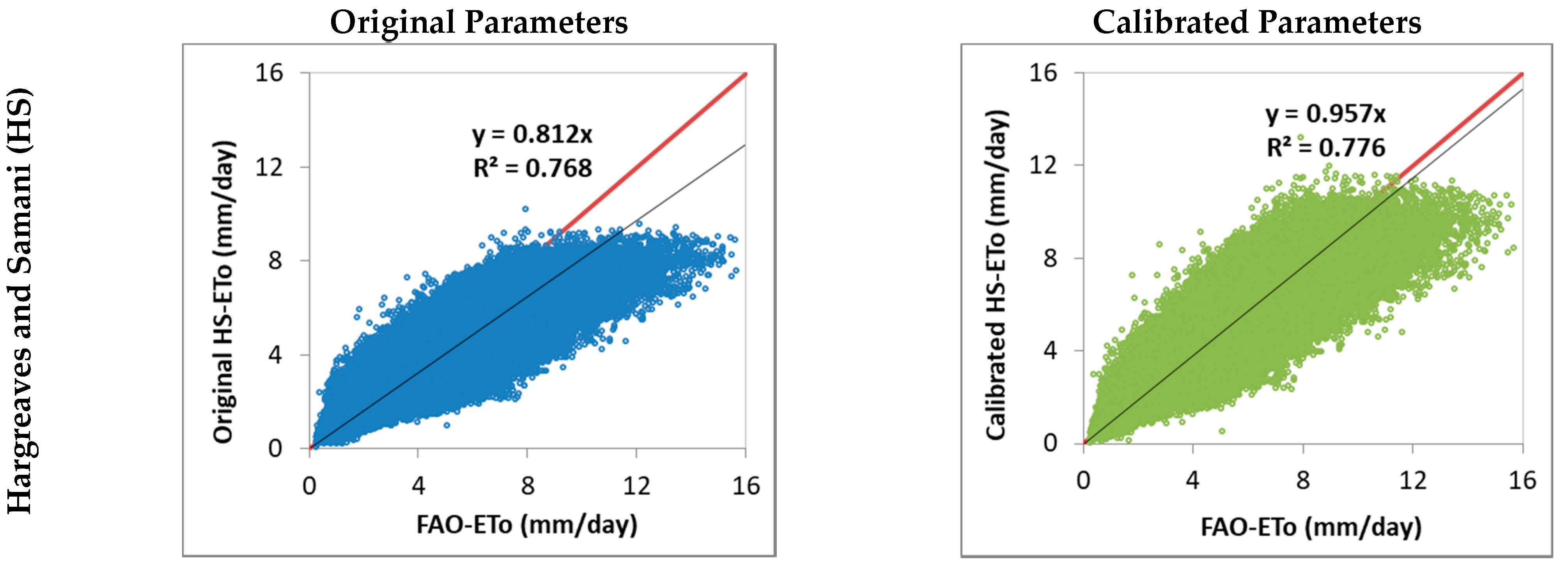
• Hargreaves and Samani (HS):

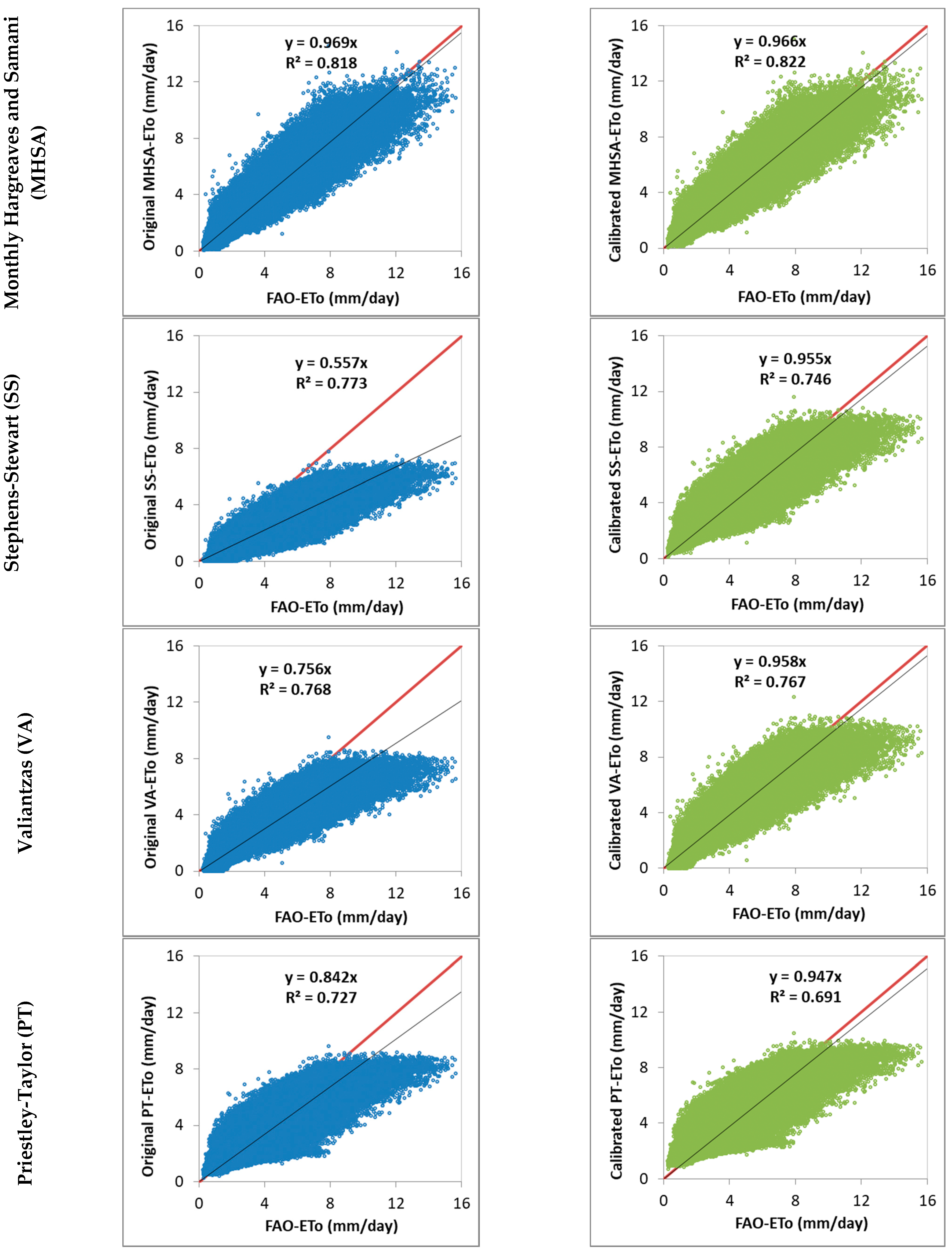
$${\mathrm{ET}}_{\mathrm{o}}=0.408a{R}_a\left(T_{avg}+b\right){\left(T_{max}-T_{min}\right)}^c$$

(2)

• Valiantzas (VA):

$${\mathrm{ET}}_{\mathrm{o}}=a{R}_s\sqrt{\left(T_{avg}+9.5\right)}-b{R}_s^{0.6}{\phi }^{0.15}+c(T_{avg}+20){\left(T_{max}-T_{min}\right)}^{0.7}$$

(3)

• Monthly Hargreaves and Samani (MHSA):

$${\mathrm{ET}}_{\mathrm{o}}=0.408a_i{R}_a\left(T_{avg}+b_i\right){\left(T_{max}-T_{min}\right)}^{c_i} i=1 to 12$$

(4)

• Priestley-Taylor (PT):

$${\mathrm{ET}}_{\mathrm{o}}=0.408a\left(\frac{\Delta }{\Delta +\gamma }\right)\left(R_n-G\right)+b$$

(5)

• Makkink (MA):

$${\mathrm{ET}}_{\mathrm{o}}=0.408a\left(\frac{\Delta }{\Delta +\gamma }\right)R_s-b$$

(6)

• Stephens-Stewart (SS):

$${\mathrm{ET}}_{\mathrm{o}}=0.408\left(a{T}_{avg}+b\right)R_s$$

(7)

where $R_a$ is the extraterrestrial radiation (MJ m⁻² d⁻¹) and calculated as detailed by following Allen et al. [9], $R_s$ is the solar radiation (MJ m⁻² d⁻¹), $R_n$ is the net radiation (MJ m⁻² d⁻¹), ∆ is the slope of vapor pressure curve (kPa °C⁻¹), γ is the psychrometric constant (kPa °C⁻¹), j is the latitude, $T_{avg}$ is calculated as the average of $T_{max}$ and $T_{min}$, and the coefficient of 0.408 was used to convert from MJ m⁻² d⁻¹ to mm d⁻¹. a, b and c are multiplier and offset parameters. For radiation-based methods (Equations (3), (6) and (7)), solar radiation ($R_s$) was estimated using Hargreaves and Samani radiation equation [27] as follows:

$$R_s=K_{Rs}{R}_a\sqrt{\left(T_{max}-T_{min}\right)}$$

(8)

where, $K_{Rs}$ is the empirical radiation adjustment coefficient. Allen et al. [9] suggested $K_{Rs}=0.16$ for ‘interior’ locations (where land mass dominates and air masses are not strongly influenced by a large water body) and $K_{Rs}=0.19$ for ‘coastal’ locations.

3.3. Evaluation Procedure

In this study, we first evaluated the results of ET_o estimated using the original parameters for Equations (1)–(7), which were compared to the FAO-PM ET_o estimates. Then, these equations were calibrated against FAO-PM ET_o using the R Package “nlstools” [28]. Finally, the computed ET_o of the six equations using calibrated parameters was compared with those of FAO-PM ET_o computed using the full datasets. To assess the performance of ET_o estimation by the empirical methods (original and calibrated) with respect to standard FAO-PM ET_o, linear regression was forced to the origin, and several statistical indicators were used. These indicators are explained below:

$$\mathrm{RMSE}=\sqrt{\frac{1}{n}{{\displaystyle \sum }}_{i=1}^n{\left(y_i-x_i\right)}^2}$$

(9)

$$d=1-\frac{{{\displaystyle \sum }}_{i=1}^n{\left(y_i-x_i\right)}^2}{{{\displaystyle \sum }}_{i=1}^n{\left(\left|y_i-\overline{x}\right|+\left|x-\overline{x}\right|\right)}^2}$$

(10)

$$\mathrm{Ratio}=\frac{{{\displaystyle \sum }}_{i=1}^n{y}_i}{{{\displaystyle \sum }}_{i=1}^n{x}_i}$$

(11)

$$b_o=\frac{n{\displaystyle \sum }{x}_i{y}_i-({\displaystyle \sum }{x}_i)\left({\displaystyle \sum }{y}_i\right)}{n{\displaystyle \sum }{x}_i^2-{\left({\displaystyle \sum }{x}_i\right)}^2}$$

(12)

$$R^2=\frac{{\displaystyle \sum }{\left(y_i-\overline{y}\right)}^2-{\displaystyle \sum }{\left(y_i-\widehat{y}\right)}^2}{{\displaystyle \sum }{\left(y_i-\overline{y}\right)}^2}$$

(13)

where n = number of available days; y_i = estimated ET_o using different equations with original or calibrated parameters and x_i = estimated ET_o using the fully parameterized FAO Penman-Monteith (FAO-PM) equation, $\overline{x}$ = average value of x_i, $\overline{y}$ = average value of y_i, $\widehat{y}$ = predicted value of y for a given x -value, and b_o = regression coefficient of the regression forced to the origin. If the coefficient of regression b_o is close to 1, then the estimated values from empirical equations are statistically close to that from the standard FAO-PM equation. When the coefficient of determination R² is close to 1.0, then most of the variation of the FAO-PM ET_o values can be explained by the model. The Root Mean Square Error characterizes the variance of the errors; the smaller the RMSE, the better the model’s performance. Willmott index of agreement (d) is a standardized measure of the degree of model estimation error, and a value of 1 indicates a perfect match. The ratio is used to quantify the under and overestimation of ET_o using different equations compared to that obtained with FAO-PM.

4. Results and Discussion

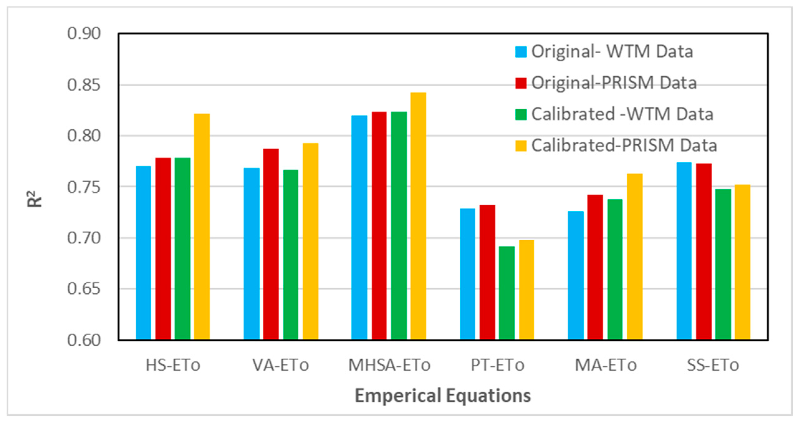
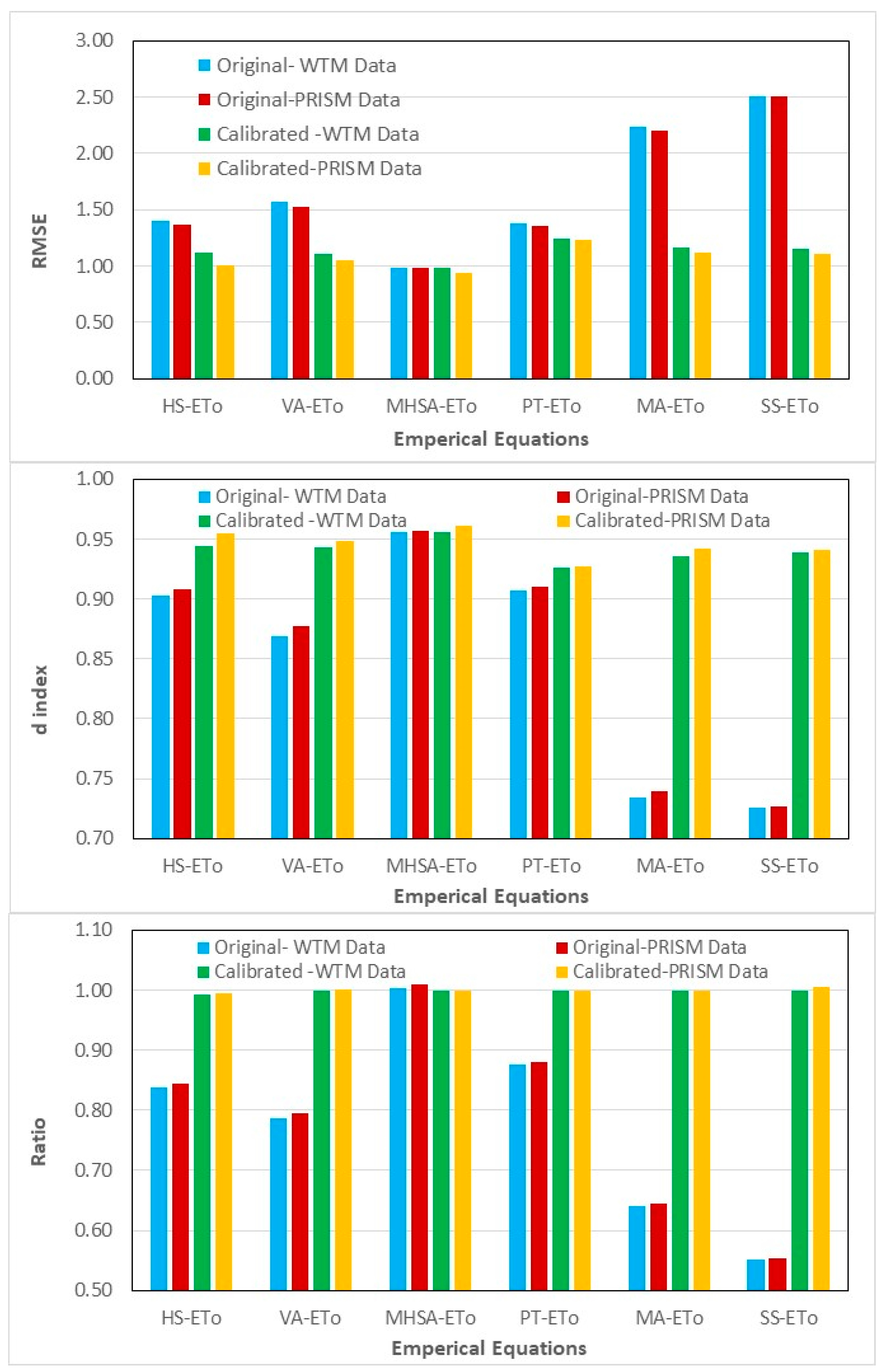
4.1. Results

The performance of all empirical equations using the original and calibrated parameters is evaluated in comparison with the FAO-PM ET_o using WTM and PRISM datasets. Figure 3 illustrates the relationship between predicted ET_o from the empirical equations and the standard FAO-PM method based on data from WTM. The departure from the straight line 1:1 in all the selected equations (R² ranged from 0.727 to 0.818 and regression coefficient ranged from 0.557 to 0.969) confirmed the unsatisfactory performance and marked tendency to underestimate ET_o. This underestimation concurs with previous studies carried out in other regions [29,30,31].

Utilizing only available limited meteorological data to enhance ET_o calculation accuracy, we calibrated the empirical equations using 10-year daily ET_o values estimated with the FAO-PM equation using weather data from 48 meteorological stations of WTM. Results of the calibration exercise (

Table 1. Original and calibrated coefficient values of the selected empirical equations.

Representative Equation		Parameter Values
	Month	Original	Calibrated
			WTM Data	PRISM Data
Hargreaves and Samani (HS)	-	a = 0.0023 b = 17.8 c = 0.50	a = 0.0014 b = 23.78 c = 0.69	a = 0.0008 b = 24.43 c = 0.88
Valiantzas (VA)	-	a = 0.0393 b = 0.19 c = 0.0037	a = 0.0457 b = 0.30 c = 0.0076	a = 0.0446 b = 0.3458 c = 0.0089
Priestley-Taylor (PT)	-	a = 1.26 b = 0	a = 1.314 b = 0.42	a = 1.314 b = 0.394
Makkink (MA)	-	a = 0.61 b = 0.12	a = 0.98 b = 0.32	a = 0.991 b = 0.423
Stephens-Stewart (SS)	-	a = 0.0148 b = 0.07	a = 0.0142 b = 0.36	a = 0.0135 b = 0.3710
Monthly Hargreaves and Samani (MHSA)	Jan	a = 0.0051 b = 10.26 c = 0.5069	a = 0.0041 b = 11.02 c = 0.564	a = 0.0015 b = 14.780 c = 0.8500
	Feb	a = 0.0045 b = 11.36 c = 0.4934	a = 0.0047 b = 11.500 c = 0.4670	a = 0.0014 b = 16.390 c = 0.8000
	Mar	a = 0.0034 b = 12.05 c = 0.5325	a = 0.0033 b = 11.790 c = 0.550	a = 0.0014 b = 16.490 c = 0.7700
	Apr	a = 0.0038 b = 9.227 c = 0.5161	a = 0.0035 b = 9.0410 c = 0.5410	a = 0.0013 b = 15.870 c = 0.8200
	May	a = 0.0034 b = 2.955 c = 0.5913	a = 0.0031 b = 2.6540 c = 0.6260	a = 0.0014 b = 6.9200 c = 0.8400
	Jun	a = 0.0069 b = −7.604 c = 0.4730	a = 0.0063 b = −7.379 c = 0.4970	a = 0.00315 b = −4.0770 c = 0.6900
	Jul	a = 0.0058 b = −6.306 c = 0.4723	a = 0.0057 b = −7.049 c = 0.4890	a = 0.0037 b = −4.343 c = 0.60
	Aug	a = 0.0061 b = −5.496 c = 0.4376	a = 0.0065 b = −5.553 c = 0.6140	a = 0.0036 b = −2.504 c = 0.580
	Sep	a = 0.0030 b = 3.159 c = 0.5939	a = 0.0030 b = 2.0110 c = 0.6060	a = 0.00187 b = 4.928 c = 0.74
	Oct	a = 0.0038 b = 8.628 c = 0.4913	a = 0.0036 b = 8.5560 c = 0.5120	a = 0.00162 b = 13.780 c = 0.720
	Nov	a = 0.0047 b = 13.87 c = 0.4126	a = 0.0040 b = 14.100 c = 0.4580	a = 0.0012 b = 23.04 c = 0.77
	Dec	a = 0.0035 b = 11.51 c = 0.5958	a = 0.0035 b = 11.840 c = 0.5930	a = 0.00128 b = 16.95 c = 0.86

) revealed the following:

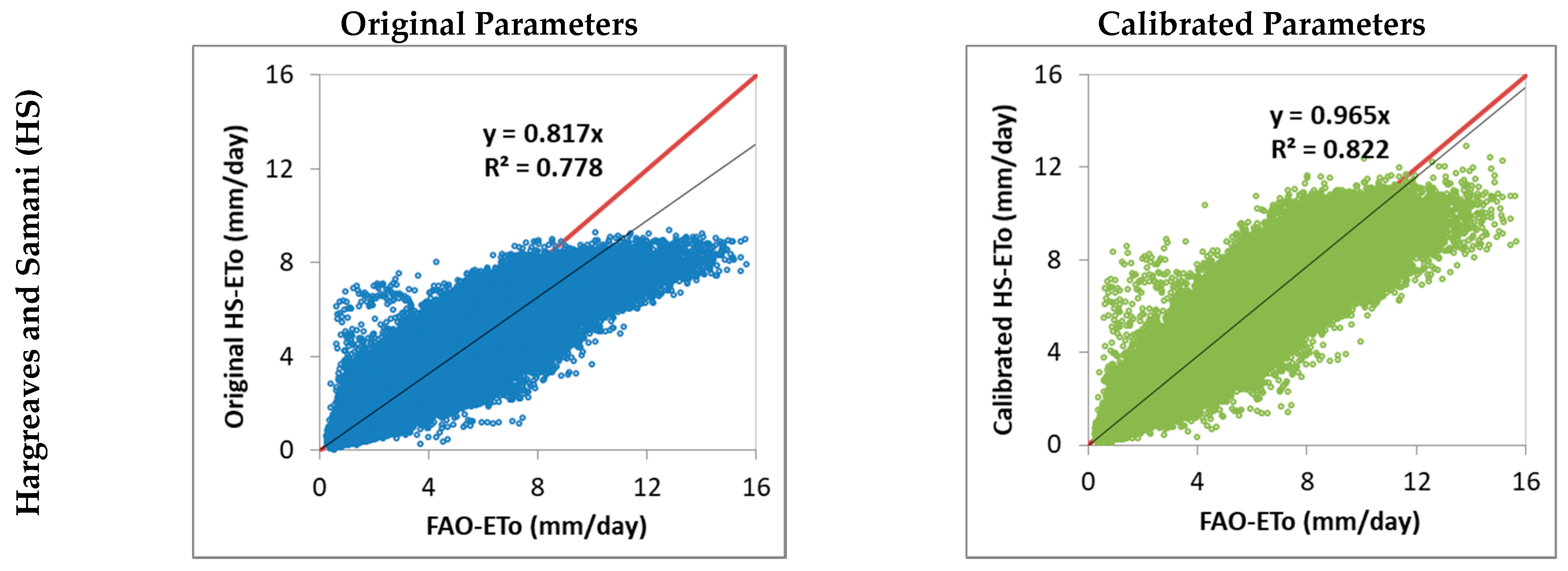
• Parameter calibration of HS equation resulted in lower coefficient “a” (0.0014 with WTM and 0.0008 with PRISM) and higher coefficients “b” (23.78 with WTM and 24.43 with PRISM) and “c” (0.69 with WTM and 0.88 with PRISM) than the original values (a = 0.0023, b = 17.8, and c = 0.5),
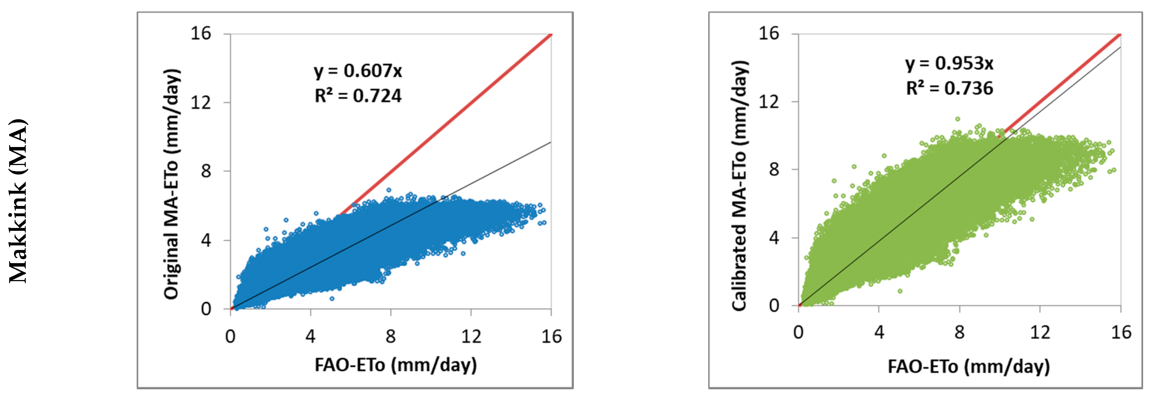
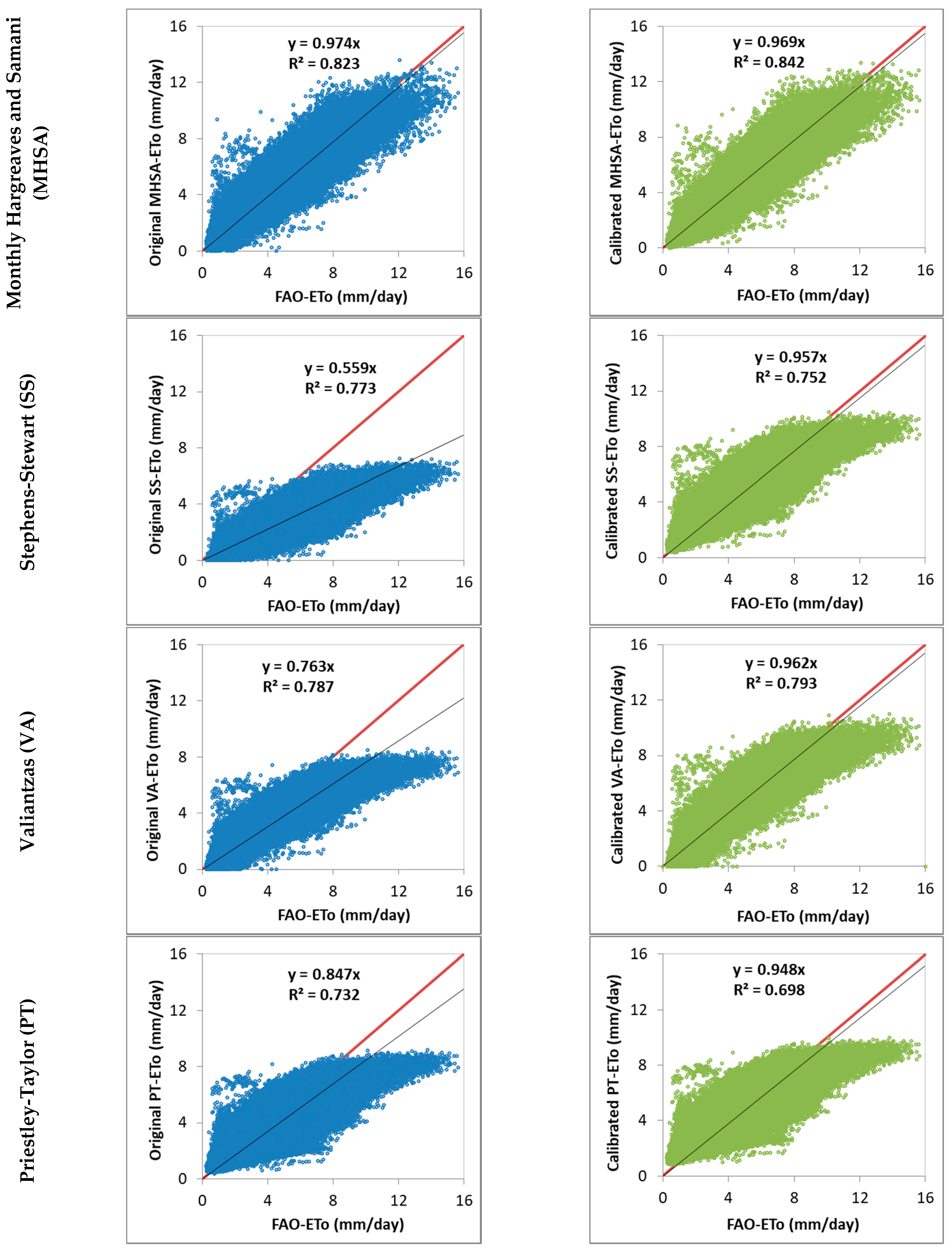
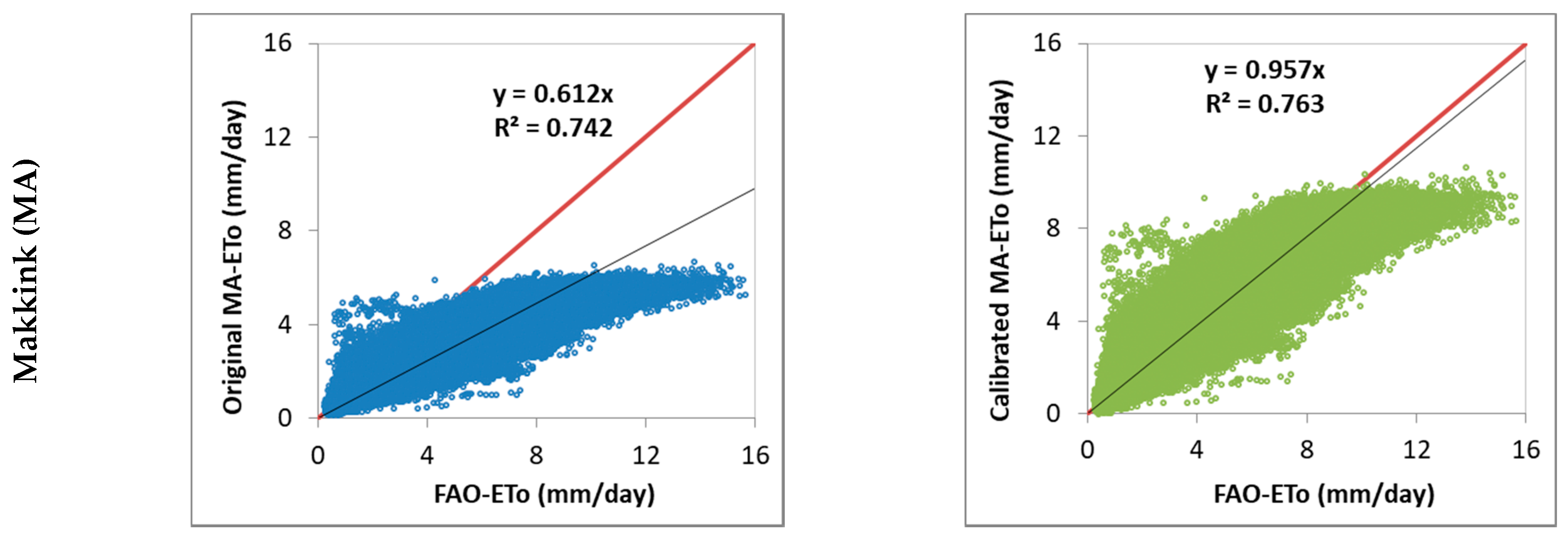
• Calibrated values of VA, PT, and MA methods are higher than their original parameters using both WTM and PRISM datasets, and
• The value of the “b” coefficient of the SS equation changed remarkably after calibration.

Empirical equations with the adjusted parameters have a better estimation of ET_o than their original parameters, as supported by the significant improvements in their correlation relationships (R² value ranging from 0.691 (PT equation) to 0.822 (MHSA equation)) and a slope value closer to one (Figure 3). A slope value less than 1 indicates that the systematic underestimation of ET_o is originated from the original empirical methods. MHSA and HS equations had the best performances as a result of the calibration process. Results of the same analysis but using PRISM datasets are depicted in Figure 4.

All methods underestimated ET_o when original parameters were used (R² ranged from 0.732 to 0.823 and regression coefficient of 0.559 to 0.974); however, ET_o estimation of all methods substantially improved (R² ranged from 0.698 to 0.842 and regression coefficient of 0.948 to 0.969) when the values of the calibrated parameters are used. MHSA had the best performance; however, all methods underestimated ET_o values in the range of 8–16 mm. Statistical indices (R², RMSE, d index, and Ratio) used to assess the performance of ET_o estimates using original and calibrated empirical equations with WTM and PRISM datasets are depicted in Figure 5. According to these results, MHSA with calibrated parameters has the best performance using PRISM (R² of 0.842, RMSE of 0.941, d index of 0.961, and Ratio of 1.005) than WTM datasets (R² of 0.823, RMSE of 0.987, d index of 0.957 and Ratio of 1.0). Also, MHSA has superior performance compared to other models with uncalibrated parameters using WTM and PRISM datasets. The MHSA equation was derived by calibrating the HS equation monthly for the same region using weather data from 2005 to 2015 [15]. The calibration data used to generate calibrated parameters for MHSA included one year more data than that used in the uncalibrated equation. This explains the similar performance of MHSA using the default and calibrated parameters. One might conclude that the performance of the empirical equations improved using the values of fitting parameters generated based on the PRISM datasets compared to the default values (Figure 5). These findings concur with results reported on research conducted in Switzerland, West Australia [32], India [33], and China [34].

4.2. Discussion

The climate of West Texas varies considerably in different parts of the study area; it includes cold semiarid, hot semiarid, hot desert, humid subtropical, and cold desert, according to Koppen’s classification. Weather data from the 48 WTM stations and 800 m resolution PRISM data of the same WTM station locations were used to estimate ET_o using selected models. Results of the calibrated MHSA (i.e., monthly calibrated HS) using PRISM datasets performed the best (based on r², RMSE, d-index, and the Ratio) compared to the other models. The second-best model is the HS model, followed by VA, MA, SS, and PT using PRISM datasets. The improved estimation of ET_o with the HS and MHSA models agrees with several other studies [35,36,37]. The least performing model was the radiation-based PT model, commonly used in crop modeling because it requires fewer climatic parameters than other models. However, the results of this study do not recommend its suitability for the study area. Literature reveals conflicting results on the performance of the PT model [33,35,38,39] in dry and wet climates. Advective energy is the main reason for its poor performance in arid climates [40] and could be the same reason for its poor performance in the present study. The PT model coefficient ‘a’ varies with time, surface type and condition (e.g., vegetation type and soil moisture condition), and micrometeorological state, including advective energy [40,41]; therefore, the model needs calibration before application.

The superior performance of MHSA could be because it accounts for seasonal variation of climatic parameters [42]. In this study, all models were calibrated without subdividing climate data based on seasons except for MHSA. Xu and Sing [43] studied the seasonal effects on ET_o estimation and found better prediction with seasonally divided datasets, which explains, at least a part, the reasons for the superior performance of the MHSA model. Also, the HS model has a less aridity-bias impact [29], which could be another reason for the better performance of MHSA (monthly calibrated HS) and HS in drier climates in West Texas. However, prediction accuracies were comparatively lower in this study than in many similar studies [35,36,38]. In the studies mentioned above, a better prediction from the models was due to analysis based on different climate regimes (humid vs. arid). In this study, during the calibration process, variability in the climatic regime was not considered station-wise, resulting in low prediction accuracy. In other words, each equation has strong correlations with the local climatic parameter settings and works best in the climate types in which it was developed initially [35,38]. However, pooling and analyzing data from a large region allowed better applicability of the models to a broader range of environmental conditions.

It is noted that the temperature-based models performed better than radiation-based models. This finding concurs with that reported by Sharafi and Ghaleni [44], who evaluated 32 different empirical equations in different Iranian climates and observed that the temperature-based ET equation predicted ET_o more accurately than the solar radiation- and mass transfer-based equations for drier climates. In drier climates, the temperature based equation gives a more accurate ET_o estimation [39], which is also observed in the present study, where the best three performing models were temperature-based. Also, ET_o prediction was better using PRISM than WTM datasets. The potential introduction of measurement or computational errors to observed data may have caused significant errors in estimated ET_o [45], or the theoretical architecture of ET_o estimation combining interpolated data and mathematical models may have resulted in this difference.

A systematic bias– underestimating high values– was observed in each model’s prediction. This systematic bias at extreme values probably is induced by the variation of climate and earth physiographic features. Variation in the climate regime (humid vs. arid) or the influence of earth physiography was not considered in the calibration phase of the present study. In contrast, Awal et al. [15] observed improvement in ET_o prediction when considering factors such as climate regime, wind speed, and elevation in calibration in West Texas. Xystrakis and Matzarakis [46] found the disappearance of constant over-or under-estimation with seasonal analysis for ET_o estimation. They suggested a change in ET_o models with seasons to avoid these systematic biases.

5. Conclusions

The reference crop evapotranspiration is used to determine crop water requirements, essential for effective irrigation scheduling programs and other water management efforts. Evaluating the performance of simple ET_o calculation methods has received considerable attention in areas where complete weather data are not readily available at the spatio-temporal scales needed to warrant the use of the FAO Penman-Monteith equation. The main objective of this study was to evaluate the performance of different empirical ET_o calculation methods under West Texas conditions.

The reference crop evapotranspiration estimated using the temperature- or radiation-based Hargreaves-Samani (HS), Monthly Hargreaves-Samani (MHSA), Valiantzas (VA), Priestley-Taylor (PT), Makkink (MA), and Stephens-Stewart (SS) equations were compared and evaluated with those estimated using the standard FAO-PM in West Texas. Calculated ET_o with all empirical methods was lower than those calculated by FAO-PM when the original values of their fitting parameters were used.

However, the performance of these empirical models improved after a calibration exercise using daily ET_o generated with the FAO-PM method. All methods underestimated FAO-PM ET_o in the range of 8–16 mm. MHSA outperformed all the methods using default or calibrated fitting parameter values with daily weather data either from WTM or PRISM. ET_o estimated using temperature- and radiation-based methods has a better performance using PRISM than WTM datasets. This study identified the best empirical method to estimate ET_o and paved the way in providing the high spatial resolution ET_o using daily PRISM data for water resources management in West Texas.

References

1. Texas Water Development Board (TWDB). 2022 State Water Plan—Water for Texas. 2021. Available online: https://www.twdb.texas.gov/waterplanning/swp/2022/docs/SWP22-Water-For-Texas.pdf (accessed on 12 July 2022).
2. USDA-NASS. 2017 Census of Agriculture, 2018 Irrigation and Water Management Survey; Special Studies, Part 1. AC-17-SS-1; USDA-NASS: Washington, DC, USA, 2019; Volume 3. Available online: https://www.nass.usda.gov/Publications/AgCensus/2017/Online_Resources/Farm_and_Ranch_Irrigation_Survey/fris.pdf (accessed on 21 December 2021).
3. Wagner, K. EM-115 Status and Trends of Irrigated Agriculture in Texas, Texas Water Resources Institute. 2012. Available online: https://twri.tamu.edu/publications/educational-materials/2012-educational-materials/em-115/ (accessed on 21 December 2021).
4. Awal, R.; Fares, A.; Habibi, H. Irrigation Scheduling Tools: IrrigWise and IrrigWise_PRISM for Agricultural Crops and Urban Landscapes. In Proceedings of the 6th Decennial National Irrigation Symposium, San Diego, CA, USA, 6–8 December 2021. [Google Scholar] [CrossRef]
5. Lima, F.A.; Martínez-Romero, A.; Tarjuelo, J.M.; Córcoles, J.I. Model for management of an on-demand irrigation network based on irrigation scheduling of crops to minimize energy use (Part I): Model Development. Agric. Water Manag. 2018, 210, 49–58. [Google Scholar] [CrossRef]
6. George, B.A. Technical Manual for “Crop Water Requirements and Irrigation Scheduling”. 2017. Available online: https://hdl.handle.net/20.500.11766/6406 (accessed on 20 December 2021).
7. Fernández, J.E.; Cuevas, M.V. Irrigation scheduling from stem diameter variations: A review. Agric. For. Meteorol. 2010, 150, 135–151. [Google Scholar] [CrossRef]
8. Awal, R.; Fares, A.; Habibi, H. Optimum turf grass irrigation requirements and corresponding water-energy-CO2 Nexus across Harris County, Texas. Sustainability 2019, 11, 1440. [Google Scholar] [CrossRef]
9. Allen, R.G.; Pereira, L.S.; Raes, D.; Smith, M. Crop evapotranspiration-Guidelines for computing crop water requirements-FAO Irrigation and drainage paper 56. FAO Rome 1998, 300, D05109. [Google Scholar]
10. Hargreaves, G.H.; Samani, Z.A. Reference crop evapotranspiration from temperature. Appl. Eng. Agric. 1985, 1, 96–99. [Google Scholar] [CrossRef]
11. Valiantzas, J.D. Simple ET0 forms of Penman’s equation without wind and/or humidity data. I: Theoretical development. J. Irrig. Drain. Eng. 2013, 139, 1–8. [Google Scholar] [CrossRef]
12. Priestley, C.H.B.; Taylor, R.J. On the assessment of surface heat flux and evaporation using large-scale parameters. Mon. Weather Rev. 1972, 100, 81–92. [Google Scholar] [CrossRef]
13. McGuinness, J.L.; Bordne, E.F. A Comparison of Lysimeter-Derived Potential Evapotranspiration with Computed Values; US Department of Agriculture: Washington, DC, USA, 1972.
14. Makkink, G.F. Testing the Penman formula by means of lysimeters. J. Inst. Water Eng. 1957, 11, 277–288. [Google Scholar]
15. Awal, R.; Habibi, H.; Fares, A.; Deb, S. Estimating reference crop evapotranspiration under limited climate data in West Texas. J. Hydrol. Reg. Stud. 2020, 28, 100677. [Google Scholar] [CrossRef]
16. Liu, X.; Xu, C.; Zhong, X.; Li, Y.; Yuan, X.; Cao, J. Comparison of 16 models for reference crop evapotranspiration against weighing lysimeter measurement. Agric. Water Manag. 2017, 184, 145–155. [Google Scholar] [CrossRef]
17. Valipour, M.; Montazar, A.A. Optimize of all effective infiltration parameters in furrow irrigation using visual basic and genetic algorithm programming. Aust. J. Basic Appl. Sci. 2012, 6, 132–137. [Google Scholar]
18. Cai, J.; Liu, Y.; Lei, T.; Pereira, L.S. Estimating reference evapotranspiration with the FAO Penman–Monteith equation using daily weather forecast messages. Agric. For. Meteorol. 2007, 145, 22–35. [Google Scholar] [CrossRef]
19. Chiew, F.H.S.; Kamaladasa, N.N.; Malano, H.M.; McMahon, T.A. Penman-Monteith, FAO-24 reference crop evapotranspiration and class-A pan data in Australia. Agric. Water Manag. 1995, 28, 9–21. [Google Scholar] [CrossRef]
20. Hssaine, B.A.; Merlin, O.; Rafi, Z.; Ezzahar, J.; Jarlan, L.; Khabba, S.; Er-Raki, S. Calibrating an evapotranspiration model using radiometric surface temperature, vegetation cover fraction and near-surface soil moisture data. Agric. For. Meteorol. 2018, 256, 104–115. [Google Scholar] [CrossRef]
21. Srivastava, A.; Sahoo, B.; Raghuwanshi, N.S.; Chatterjee, C. Modelling the dynamics of evapotranspiration using Variable Infiltration Capacity model and regionally calibrated Hargreaves approach. Irrig. Sci. 2018, 36, 289–300. [Google Scholar] [CrossRef]
22. Trajkovic, S. Temperature-based approaches for estimating reference evapotranspiration. J. Irrig. Drain. Eng. 2005, 131, 316–323. [Google Scholar] [CrossRef]
23. Yin, Y.; Wu, S.; Zheng, D.; Yang, Q. Radiation calibration of FAO56 Penman–Monteith model to estimate reference crop evapotranspiration in China. Agric. Water Manag. 2008, 95, 77–84. [Google Scholar] [CrossRef]
24. TWDB. Water for Texas. 2012. State Water Plan. 2012. Available online: http://www.twdb.texas.gov/publications/state_water_plan/2012/2012_SW.P.pdf (accessed on 21 December 2021).
25. Schroeder, J.L.; Burgett, W.S.; Haynie, K.B.; Sonmez, I.; Skwira, G.D.; Doggett, A.L.; Lipe, J.W. The West Texas mesonet: A technical overview. J. Atmos. Ocean. Technol. 2005, 22, 211–222. [Google Scholar] [CrossRef]
26. PRISM Climate Group, Oregon State University. Available online: https://prism.oregonstate.edu (accessed on 21 December 2021).
27. Hargreaves, G.H.; Samani, Z.A. Estimating potential evapotranspiration. J. Irrig. Drain. Div. 1982, 108, 225–230. [Google Scholar] [CrossRef]
28. Baty, F.; Ritz, C.; Charles, S.; Brutsche, M.; Flandrois, J.-P.; Delignette-Muller, M.-L. A toolbox for nonlinear regression in R: The package nlstools. J. Stat. Softw. 2015, 66, 1–21. [Google Scholar] [CrossRef]
29. Hargreaves, G.H.; Allen, R.G. History and evaluation of Hargreaves evapotranspiration equation. J. Irrig. Drain. Eng. 2003, 129, 53–63. [Google Scholar] [CrossRef]
30. Valero, J.F.M.; Álvarez, V.M.; Real, M.M.G. Regionalization of the Hargreaves coefficient to estimate long-term reference evapotranspiration series in SE Spain. Span. J. Agric. Res. 2013, 11, 1137–1152. [Google Scholar] [CrossRef] [Green Version]
31. Berengena, J.; Gavilán, P. Reference evapotranspiration estimation in a highly advective semiarid environment. J. Irrig. Drain. Eng. 2005, 131, 147–163. [Google Scholar] [CrossRef]
32. Ahooghalandari, M.; Khiadani, M.; Jahromi, M.E. Calibration of Valiantzas’ reference evapotranspiration equations for the Pilbara region, Western Australia. Theor. Appl. Climatol. 2017, 128, 845–856. [Google Scholar] [CrossRef]
33. Rahimikhoob, A.; Behbahani, M.R.; Fakheri, J. An evaluation of four reference evapotranspiration models in a subtropical climate. Water Resour. Manag. 2012, 26, 2867–2881. [Google Scholar] [CrossRef]
34. Feng, Y.; Jia, Y.; Cui, N.; Zhao, L.; Li, C.; Gong, D. Calibration of Hargreaves model for reference evapotranspiration estimation in Sichuan basin of southwest China. Agric. Water Manag. 2017, 181, 1–9. [Google Scholar] [CrossRef]
35. Gao, F.; Feng, G.; Ouyang, Y.; Wang, H.; Fisher, D.; Adeli, A.; Jenkins, J. Evaluation of reference evapotranspiration methods in arid, semiarid, and humid regions. JAWRA J. Am. Water Resour. Assoc. 2017, 53, 791–808. [Google Scholar] [CrossRef]
36. Martınez-Cob, A.; Tejero-Juste, M. A wind-based qualitative calibration of the Hargreaves ET0 estimation equation in semiarid regions. Agric. Water Manag. 2004, 64, 251–264. [Google Scholar] [CrossRef]
37. George, B.A.; Reddy, B.R.S.; Raghuwanshi, N.S.; Wallender, W.W. Decision support system for estimating reference evapotranspiration. J. Irrig. Drain. Eng. 2002, 128, 1–10. [Google Scholar] [CrossRef]
38. Tabari, H. Evaluation of reference crop evapotranspiration equations in various climates. Water Resour. Manag. 2010, 24, 2311–2337. [Google Scholar] [CrossRef]
39. Nandagiri, L.; Kovoor, G.M. Performance evaluation of reference evapotranspiration equations across a range of Indian climates. J. Irrig. Drain. Eng. 2006, 132, 238–249. [Google Scholar] [CrossRef]
40. Arasteh, P.D.; Tajrishy, M. Calibrating Priestley-Taylor model to estimate open water evaporation under regional advection using volume balance method-case study: Chahnimeh reservoir, Iran. J. Appl. Sci. 2008, 8, 4097–4104. [Google Scholar] [CrossRef]
41. Fisher, J.B.; DeBiase, T.A.; Qi, Y.; Xu, M.; Goldstein, A.H. Evapotranspiration models compared on a Sierra Nevada forest ecosystem. Environ. Model. Softw. 2005, 20, 783–796. [Google Scholar] [CrossRef]
42. Júnior, L.C.G.V.; Ventura, T.M.; Gomes, R.S.R.; de Nogueira, J.S.; de Lobo, F.A.; Vourlitis, G.L.; Rodrigues, T.R. Comparative assessment of modelled and empirical reference evapotranspiration methods for a Brazilian savanna. Agric. Water Manag. 2020, 232, 106040. [Google Scholar] [CrossRef]
43. Xu, C.-Y.; Singh, V.P. Cross comparison of empirical equations for calculating potential evapotranspiration with data from Switzerland. Water Resour. Manag. 2002, 16, 197–219. [Google Scholar] [CrossRef]
44. Sharafi, S.; Ghaleni, M.M. Calibration of empirical equations for estimating reference evapotranspiration in different climates of Iran. Theor. Appl. Climatol. 2021, 145, 925–939. [Google Scholar] [CrossRef]
45. Meyer, S.J.; Hubbard, K.G.; Wilhite, D.A. Estimating potential evapotranspiration: The effect of random and systematic errors. Agric. For. Meteorol. 1989, 46, 285–296. [Google Scholar] [CrossRef]
46. Xystrakis, F.; Matzarakis, A. Evaluation of 13 empirical reference potential evapotranspiration equations on the island of Crete in southern Greece. J. Irrig. Drain. Eng. 2011, 137, 211–222. [Google Scholar] [CrossRef] [Green Version]
Figure 1. (a) Texas elevation map and its climate divisions; (b) mean annual precipitation; (c) mean annual maximum temperature; and (d) mean annual minimum temperature.
Water 14 03032 g001
Figure 2. (a) Active weather station network across Texas; (b) locations of 48 WTM weather stations used in the analysis.
Water 14 03032 g002
Figure 3. Relationship between estimated ETo by the selected empirical methods and FAO-PM using WTM weather data.
Water 14 03032 g003aWater 14 03032 g003bWater 14 03032 g003c
Figure 4. Relationship between estimated ETo by the selected empirical methods and FAO-PM using high-resolution PRISM weather data.
Water 14 03032 g004aWater 14 03032 g004bWater 14 03032 g004c
Figure 5. Performance of estimation of ETo from the selected empirical equations against the standard method.
Water 14 03032 g005aWater 14 03032 g005b