Abstract
The water harvesting potential of atmospheric water generators (AWGs) in high-altitude semiarid regions can be diminutive relative to the water generation capacity. Operational parameters for the dehumidification process can be augmented to increase atmospheric water in the defined zone available for harvesting. In this paper, the feasibility of augmenting the microclimates of AWGs at the point of air extraction through an evaporative cooling system (ECS) was investigated. Water yield and capacity utilisation were measured from two AWGs piloted on a plant in Ga-Rankuwa, South Africa. This was implemented between December 2019 and May 2021. The study revealed that although the ECS did impact the operating parameters through decreasing temperature and increasing relative humidity (p < 0.05), variance in water yield was not significant (p > 0.05). Capacity utilisation of the AWGs remained below 50% after augmentation. Cooling efficiency of the ECS ranged between 1.4–74.5%. Energy expenditures of 0.926 kWh/L and 0.576 kWh/L for AWGs 1 and 2 were required under pristine conditions, respectively. Under the modified conditions, energy expenditure decreased to 0.855 kWh/L for AWG 1, but increased/L to 0.676 kWh for AWG 2. ECS is deduced to not be a feasible intervention for augmenting water harvesting potential for AWGs in this semiarid zone.
1. Introduction
South Africa has been forecasted to experience physical water scarcity by the year 2025 with an annual freshwater availability below the index of water scarcity, 1000 m3 per capita [1]. The Food and Agriculture Organization of the United Nations estimated present total renewable water resources in South Africa between 2018 and 2022 at 888.5 m3/inhabitant/year. This is an indication that available renewable water resources are already below the index of water scarcity. Water demand is expected to rise to 17.7 billion m3 in 2030, while water supply is projected at 15 billion m3, representing a 2.7–3.8 billion m3 water deficit [2]. Alternative water sources should be prioritised in water resource management strategies to ensure future water security.
Atmospheric water harvesting has been recognised as a method for decentralised water production that is viable for augmenting water supply [3,4,5]. Atmospheric water is a vast renewable reservoir of water, with an estimated 12,900 km3 of renewable water [6]. Atmospheric water exists in three types: clouds in the sky, fog close to the land, and vapour in the air, and collectively accounts for approximately 0.04% of total freshwater sources [7]. Devices that harvest water from the atmosphere are atmospheric water generators (AWGs). Methods for harvesting atmospheric water and advances in the technologies applied have been extensively reviewed by Tu et al. [8,9]. In dew condensation AWGs, the upper limit of dew yield is 0.8 kg/day/m2, based on radiation cooling capacity for condensation. However, in semiarid climates, the maximum observed dew water outputs typically fall within 0.3–0.6 kg/day/m2 [10]. Thus, notably, although AWGs can be used in arid and semiarid areas with low moisture content and water harvesting [11], the potential of AWGs in these areas can be diminutive relative to water generation capacity.
It is a prevailing rule that AWGs operating under a cooling condensation process do not work efficiently when the temperature falls below 18.3 °C or the relative humidity drops below 30% [12]. Shafeian et al. [13] précised hybrid AWG systems as being critical in increasing water productivity and achieve desired efficiency. Auxiliary systems to increase relative humidity were amongst those included. Pokorny et al. [14] prototyped an AWG specifically designed for arid climates. Water harvesting rate was reported from 0.23 kg/h to 1.45 kg/h.
Evaporative cooling is a passive cooling strategy which has exhibited potential as an auxiliary system. Hot and dry ambient air enters with the negative pressure effect created inside the sump interior and evaporates the water while passing through the wet pads. Through this manner, the dry-bulb temperature of the air entering the ECS decreases, and relative humidity rises [15].
Al Jubury and Hind [16] presented an indirect–direct cooling design to protect plants inside a greenhouse located in a desert climate. Greenhouse temperature decreased by ~12.1 °C and relative humidity increased from 8% to 62% compared to ambient conditions. Applications further include humidity control in processing plants, air compressor rooms, and various commercial buildings. Literature shows that depending on application and climatic conditions, evaporative cooling systems can continuously be redesigned to achieve better cooling performance [17].
In South Africa, theoretical studies on the design and simulated performance of AWGs in coastal areas have been conducted by Thisani et al. [18] and Giyaya [19]. However, empirical field studies are yet to be conducted. In tandem, at the time of this study, active ECS had not been studied or deployed as a potential auxiliary system for atmospheric water harvesting methods. This study presents an investigation of the feasibility of utilising evaporative cooling as an auxiliary system to augment the microclimate of AWGs to increase water productivity. The first stage of the research was to carry out climatological profiling of the study area to determine the environmental conditions and the forecasted baseline performance of AWGs under pristine conditions. In the second stage, an evaluation of the performance of AWGs under a modified ECS system was conducted. In addressing the performative limitations of moderately low relative humidity in the study area, it was hypothesised that the operating window for the AWGs would increase. Relative to pristine ambient weather conditions, the detected microclimate would be above the efficiency threshold for a longer period and thus, favourable in increasing water productivity.
2. Materials and Methods
2.1. Study Area and Climatological Profiling
This research was conducted in the Ga-Rankuwa Industrial area. Ga-Rankuwa is a settlement with an area of approximately 52.12 km2, and is home to an estimated population of 68,767 as last recorded in 2012 [20]. It borders two provinces, Gauteng and North West in South Africa. Gauteng is situated on the Highveld, which is high-altitude, with an elevation of 1500 m above sea level. The province is characterised by a grassland biome in the south and savanna in the north [21]. The North West province falls within the grassland and savanna biomes and is made up of flat plains and scattered trees. Ga-Rankuwa has a semiarid climate with temperature ranging from 5 to 29 °C over the course of the year. The warm season occurs from September to March, lasting for 5.8 months, and has an average daily temperature above 27 °C. The cold season occurs from May to August, lasting 2.2 months, and has an average daily temperature below 21 °C. Ga-Rankuwa experiences significant variation in rainfall, with an annual rainfall of 282 mm. January is the month which experiences the most rainfall, with an average rainfall of 94 mm. The annual average humidity in Ga-Rankuwa is 50%.
The humidity ratio or specific humidity of the study area was determined in Engineering Equation Solver (EES) –F-chart software (version 10.521) using the equation W = Mw/Mda [22]. This is illustrated in Figure 1. At 15 °C, the minimum operational temperature required for the AWGs to generate water, the specific humidity was determined to be 0.006 kg of vapour per kg of dry air.
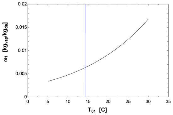
Figure 1.
Specific humidity of air in the study area.
A typical meteorological year (TMY) indicator of the temperature and relative humidity profile of the study area was developed using climate simulation model data. This data were sourced from the meteorological service Meteoblue. The time period used was from 2015 to 2020 to ensure that the simulation data used to derive the TMY were the latest and would present an updated simulation of present climate conditions of the study area. Temperature and relative humidity were the parameters used. The resulting TMY is listed below in Figure 2. A water generation profile showing how much water can be expected to be generated in the study area over a specific period under the present prevailing climate conditions of the study area was developed from the TMY. Net water generation was forecasted at 302,235 L. Water yield from an AWG consistently operating under optimal conditions (27 °C, 60% RH) was equivalent to 1,778,700 L per year. Forecasted capacity utilisation of the AWGs in the study area equated to 17%.
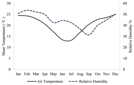
Figure 2.
Temperature and relative humidity profile in Ga-Rankuwa.
2.2. Experimental Setup
Two commercially available vapour compression cycle AWGs manufactured by Bestway Technology Co., Ltd. in Shanghai, China were commissioned on a pilot plant in Ga-Rankuwa Industrial. The extraction of water from the humid ambient air by the AWGs was achieved through the operating principle of a vapour-compression refrigeration system. The atmospheric air first passes through the cool surface of the evaporator that decreases the air temperature below the ambient dew point temperature. As a result, condensate forms on the surface of the evaporator coils. The released sensible and latent heat is absorbed by the refrigerant inside the tubes of the heat exchanger. The fresh water gathers in a collection duct under the evaporator. It is worthy to note that the amount of water extracted depends heavily on the size and design of the harvesting system. Figure 3 illustrates the operational design of the AWGs under pristine conditions and modification during the study. The specifications of the atmospheric water generators are listed in Table 1.
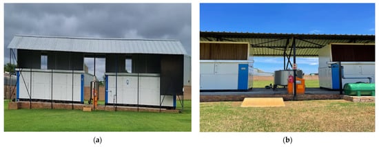
Figure 3.
Operational setup of AWGs at the site of study under (a) pristine conditions and (b) modification (ECS).

Table 1.
Specifications and operating parameters of AWGs used in the study.
Under modification, a direct cooling system was erected atop the air inlet of the AWGs. This comprised of a sump constructed around Munters’ MI-T-edgTM chemically treated cellulose-based CELdek® evaporative cooling pads. Groundwater was pumped and circulated using a circulating pump to saturate the evaporative cooling pads. Subsequently, the water accumulated in the return gutter and was recirculated. The design did not include a bleed-off system. This is summarised in the schematic diagram illustrated in Figure 4. Direct evaporative cooling systems only work properly when using once-through supply air; therefore, air was released through the AWG exhaust fans.
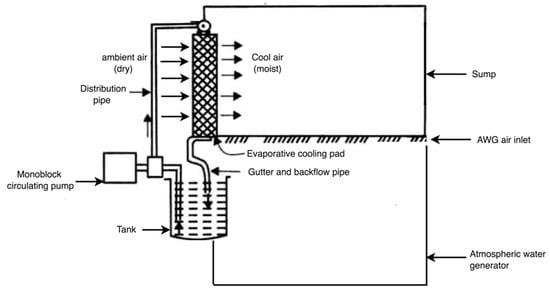
Figure 4.
Schematic diagram of evaporative cooling system.
The working principle makes use of enthalpy of vaporisation to increase humidity while reducing dry-bulb temperature [23]. Warm ambient air enters the cellulose-based pad which is sprayed with water at the wet-bulb temperature of the inlet air. Heat transfer is realised from the warm air to the cold water. The heat is transferred by the air stream as sensible heat and is absorbed by the water as latent heat. Corresponding to the value of latent heat, water is evaporated and embedded by diffusion into the flowing air, increasing the moisture content of this air. The temperature of the outlet air decreases due to the sensible heat transferred by the air [24].
The AWGs’ apparent water yield was estimated using a water generation performance sheet interpolated from data supplied by the original equipment manufacturer (OEM) as seen in Figure 5. At correlating temperature and relative humidity values, water yield from the AWGs was forecasted. At temperatures below 15 °C and relative humidity below 30%, water generation was not quantifiable and was considered negligible. When the parameters exceeded a temperature of 15 °C and relative humidity of 30%, water generation was quantifiable. A formula for forecasting water to be generated by each atmospheric water generator on a day of observation was developed based on OEM’s water generation sheet. Forecasts were generated daily using hourly temperature and relative humidity forecasts of the study area. Weather forecast data utilised in this study were sourced from the South African Weather Service and Time and Date. Forecasts of water generation from TMY and real-time weather forecasts were overlaid on measured water generation from each AWG on corresponding days. Volume of water produced (measured in litres) was represented on the radial axis and the day on the angular axis. This was to illustrate the variance in water productivity based on historic and real-time weather conditions. Forecasted water yield and measured water yield were referred to as apparent water yield and real water yield, respectively.
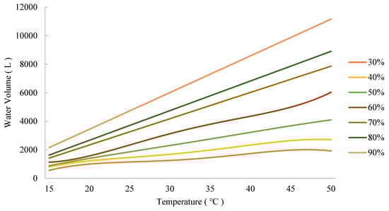
Figure 5.
Interpolated harvesting profile of AWGs at specific RH profiles.
Ambient temperature and relative humidity detected by the on-board hygrometric sensor of AWGs were read from the human–machine interface and recorded hourly. The volumetric flow of water generated by each AWG was respectively measured by a positive displacement meter. This was recorded hourly. The data set was collected over the span of one year 5 months, between December 2019 and May 2021. The data can be categorised into the following sub-categories:
- 18 December 2019–20 February 2020: data collected under pristine conditions to establish baseline performance;
- 1 March 2020–17 March 2021: data collected under modification;
- 18 March 2021–10 May 2021: data collected from one AWG unit operating under pristine conditions and the second AWG unit operating under modification.
A test of significance was conducted from the collected data. The paired t-test was the statistical method utilised to conduct a comparative analysis to determine whether the difference in specific water production per day per unit collector area from the AWGs under different operating conditions was significant. The significance threshold was set at 0.05.
Cooling efficiency of the evaporative cooling system was determined using the equation below, where Tdo is the dry-bulb temperature of the outside air, Tdin is the dry-bulb temperature of cooled air exiting the evaporative pad, and Two is the wet-bulb temperature of the ambient air [22].
3. Results
3.1. Performance of the AWGs under Pristine Conditions
The comparative relationship between the apparent and real water yield is shown in Figure 6. In December, the apparent yield calculated based on the climate profile of the study area exceeded real water yield from both AWG units. The degree in variability between the apparent and real water yield was observed to decline in January and February, respectively, relative to December. Variance was observed in the volume of water generated by each AWG unit when operating under similar conditions. This difference in real water yield was present on each day when water yield was measured. Apparent capacity utilisation for December was calculated to be 29%. During this period, capacity utilisation for AWGs 1 and 2 was measured at 13% and 19%, respectively. In January, capacity utilisation was calculated to be 31%, whereas the measured capacity utilisation was recorded at 12% and 25% for AWGs 1 and 2, respectively. Similarly, for February, capacity utilisation was calculated to be 31%, whereas the measured capacity utilisation was recorded at 25% and 42% for AWGs 1 and 2, respectively.
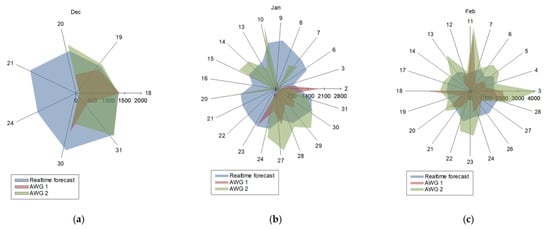
Figure 6.
Comparison between apparent and real water yield under pristine conditions during the months of (a), December 2019; (b) January 2020; and (c) February 2020.
3.2. Performance of the AWGs under Modified Conditions
The comparative relationship between the apparent and real water yield is shown in Figure 7. As seen in the baseline test, the AWGs did not generate water at an equivalent rate. Daily recorded water yield was recorded at different volumes for each AWG. Contrary to the observations noted in the baseline test, under modification, AWG 1 generated more water than AWG 2. This trend was characteristic in each month; however, the trend was most notable in October, November, and December 2020. This performance was not consistently observed during the observation period. In the results, days were observed whereby AWG 2 generated more water than AWG 1. These were noted in each individual month of observation. To better understand causation of variability in water yield, a 30-day sample size was used to determine Mean ± SD of the operational parameters. For temperature, Mean ± SD was 19.13 ± 3.4 and 18.81 ± 3.2 for AWGs 1 and 2, respectively. For relative humidity, Mean ± SD was 56.37 ± 9.5 and 57.98 ± 10.3 for AWGs 1 and 2, respectively.
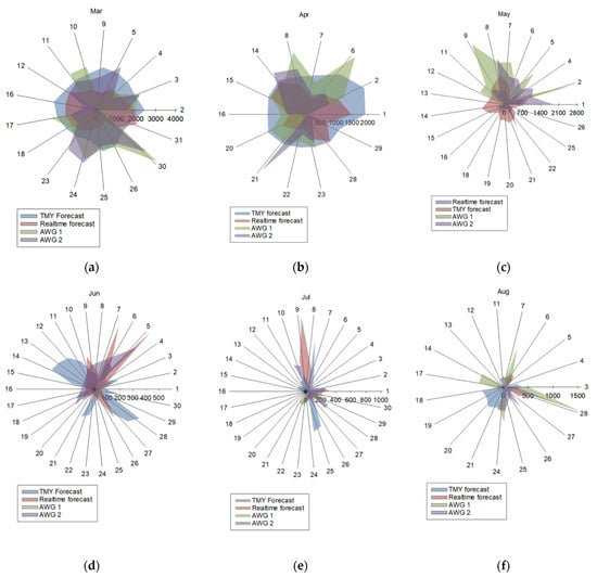
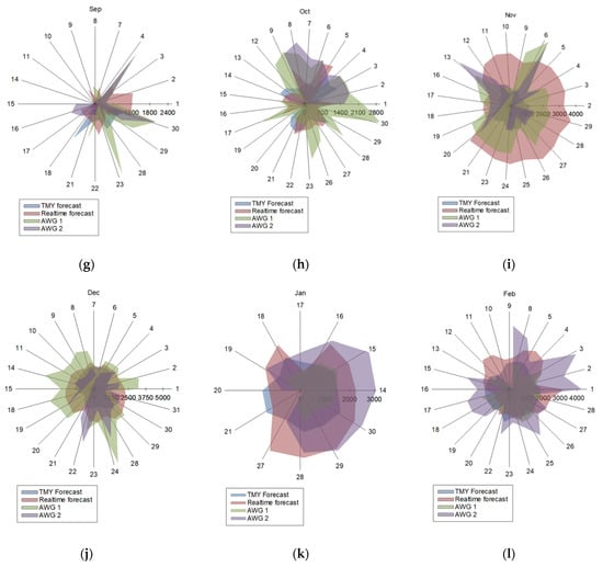
Figure 7.
Comparison between apparent and real water yield under modified conditions during the months of (a), March 2020; (b) April 2020; (c) May 2020; (d), June 2019; (e) July 2020; (f), August 2020; (g), September 2020; (h) October 2020; (i), November 2020; (j), December 2020; (k) January 2021; and (l) February 2021.
In March 2020, apparent water yield based on the TMY of the study area exceeded the apparent water yield forecasted by ambient conditions. The mean variance was recorded at 761 L. This trend continued steadily in the months of April and May. A decline was noted from June to August, with the mean variance ranging from 52 L, 27 L, and 42 L during this period. It was observed that from September, the variance in apparent water yield changed, whereby variance was determined to be −151 L, illustrating apparent water yield based on ambient conditions exceeding calculated water yield based on TMY data. This shift continued to be observed from September to March 2021. The highest mean variance was determined to be in November 2020 at 1722 L. From December, mean variance was shown to have declined. The lowest mean variance during the peak water generation period was determined to be in October 2020 at −68 L. Real water yield and capacity utilisation of the AWGs under modified conditions are summarised in Table 2.
Table 2.
Performance of the AWGs under ECS.
The average water yield for AWG 1 operating under pristine conditions and modified conditions were measured at 815.5 L and 882.6 L, respectively. The average water yield for AWG 2 operating under the pre-defined conditions were measured at 1309.6 L and 1117.6 L, respectively. The p-value was determined to be 0.693 for AWG 1 and 0.291 for AWG 2. These were above the defined significance threshold.
Figure 8 summaries water yield from AWGs operating concurrently under exposure to similar ambient conditions. AWG 2 was operating under modified conditions and AWG 1 was operating under pristine conditions. From the results, in the month of March, apparent water yield based on forecasted ambient conditions exceeds the area of apparent water yield based on TMY. Apparent water yield based on TMY exceeded apparent water yield based on forecasted ambient conditions in April.
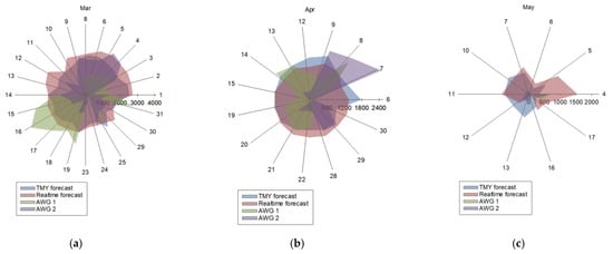
Figure 8.
Comparison between water yield from AWGs operating concurrently under pristine and modified conditions during the months of (a), March 2021; (b) April 2021; and (c) May 2021.
The average temperatures for AWGs 1 and 2 were measured at 20.8 °C and 19.9 °C. The variances for AWGs 1 and 2 were determined to be 10.6 and 7.8, respectively. The p-value was determined to be 0.163. The average relative humidity for AWGs 1 and 2 was measured at 61.8% and 66.5%. The variances for AWGs 1 and 2 were determined to be 198.8 and 187.4, respectively. The p-value was determined to be 0.145. The results from the statistical test are illustrated in Figure 9.
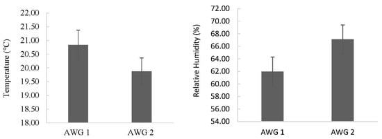
Figure 9.
Temperature and RH of AWGs operating under pristine and modified conditions.
4. Discussion
Water yield calculated from the TMY exceeded water yield calculated from present-day weather forecast data. Inter-annual variability analysis of temperature and relative humidity indicated temporal variation. Annual temperature cooling rate in the study area was −1.23 °C and relative humidity increased by 6.15%. Bosilovich et al. [20] tested the evolution of the hydrologic cycle using several 50-year model simulations. The study reported that although the water cycle is intensifying, the residence time of water increased. It is thereby implicit that the global cycling rate of water is decreasing. Kadhim et al. [25] studied a potable atmospheric water generator at a small laboratory scale. It was concluded that the volume of water extracted increased as air temperature and RH increased. This coincided with the computed performance profile of the AWGs. Shahrokhi and Esmaeil [26] sought to optimise relative humidity based on the heat transfer terms. Their observations included noting that increasing atmospheric moisture at a constant temperature would raise the amount of water harvested. In contrast, these results show that when temperature decreases and relative humidity increases, annual water harvesting potential and productivity will decline. This coincided with the computed performance profile of the AWGs and was observed in the annual water yield under ambient conditions relative to the TMY’s water yield. Assuming a continued trend in the annual temperature rate, it is to be postulated that water harvesting potential in the study area is forecasted to decline over time under pristine conditions.
4.1. Effect of Modification on AWG Parameters
The test of significance conducted shows that the differences in the operational parameters of the AWGs resulting from augmenting the microclimates through evaporative cooling are significant. This applies to both temperature and relative humidity. A steady decline in temperature was characterised as relative humidity increased. In contrast, the finding of the test of significance conducted on water yield for AWGs 1 and 2 reported that changes in water yield were not significant.
Referenced in Section 3.2, AWG 1 yielded a higher water productivity compared to AWG 2 whilst operating under similar conditions. The variability trend in water yield is hypothesised to be resultant from variation in spatial distribution of meteorological variables. An analysis of temperature and RH distribution along the ECS length, width, and height was beyond the scope of the present study. In studies where ECS was deployed, the distribution of microclimate variables within closed systems is influenced by the ambient dry-bulb temperature, relative humidity, and factors such as the ventilation system, air leakage, and thermal insulation [27]. An operational characteristic of ECSs has been outlined in the literature, where variation in the spatial temperature and relative humidity was created as a result of air movement along the direction of exhaust fans [28].
The trend in capacity utilisation continued to be significantly low under the augmented environment. The highest capacity utilisation under modification was recorded in December 2020 at 41% for AWG 1. It was thus inferred that the study area was not favourable for the optimal capacity utilisation of the AWG units, moreover, under this experimental design. Continuous operation of the ECS was observed to have a negative influence on water generation capacity within a specified day or time period. This is primarily attributed to diurnal and seasonal variations in temperature. Operating the ECS during the daytime in high-temperature months had a positive effect which resulted in increased water generation. Temperature would decline, whilst RH increased. During high-temperature periods, hourly temperatures measured at daily maximums exceeding 30 °C and, respectively, RH below 30%, were characteristic. When operating the ECS, water was produced during time intervals where water yield was forecasted as negligible under pristine conditions. This was most notable between the months of September and March. In contrast, during cooler nights where atmospheric temperature was measured to be below 18 °C, it was observed that the temperature drop which occurred due to the ECS would result in a temperature drop that was unfavourable for water generation. Water generation would, thus, be negligible. This trend was also observed during the lower-temperature months between May and August. This impact was evident in June 2020 and July 2020, where capacity utilisation was recorded at 1% for AWG 1 and AWG 2 in June, and 1% and 2%, respectively, in July. This impact was further observed in water generation trends in January and February during and subsequent to tropical cyclone Eloise.
The results obtained for the months of April, May, August, and September 2020 were used to make comparisons of cooling efficiency and temperature depression trends obtained using ECS and other evaporative cooling technologies as seen in Table 3. It must be noted that prior research applications of ECS have not been utilised in atmospheric water harvesting technologies. Previous applications have been in agriculture in the regulation of the microclimates of greenhouses and broilers. It was from this backdrop that this study was conducted to evaluate the feasibility of applying ECS in atmospheric water harvesting.
Table 3.
Comparison of ECS performance in evaporative cooling applications.
The comparisons made in Table 3 show that cooling efficiencies obtained by previous ECS applications are mainly above 35% when water-spray ECS, Fan-pad ECS, and evaporative cooling pad systems are used. Maximum cooling efficiency was 91.4% and the lowest efficiency of 38.5% was obtained in that regard. The high efficiencies reported in previous studies were attributed to the high ambient temperatures of the influent air. In this study, April, May, August, and September were the seasonal transition months where changes in climate variables and water productivity were best evident, hence explaining why these were used in the comparative study. Cooling efficiencies in the four months were lower than 35%, with the lowest cooling efficiencies measured in September. In April, the efficiency was higher than 35% (74.5%), but this is because of the combination of the high air influent temperature (18 °C) and humidity (72%). In general terms, relative to the cooling efficiency exhibited in previous applications, the introduction of evaporative cooling systems in this study as an auxiliary system did not make any substantial improvements.
4.2. Energy Consumption and Cost
During the atmospheric water harvesting process, energy expenditure varied substantially throughout the year. This is attributed to the variability of changes in humidity and temperature, as elaborated in the previous sections. Average energy consumption and subsequent cost are tabulated in Table 4. Energy expenditure was calculated based on energy consumption—off peak, energy consumption—standard, and energy consumption—peak, as determined by Eskom, the Electricity public utility of South Africa. The cost of energy in South Africa for industrial purposes is based on several factors. These include administration charge, network capacity charge, network demand charge (peak and standard), ancillary service charge, low season peak energy charge, low season standard energy charge, low season off-peak energy, affordability subsidy, electrification and rural subsidy, and a service charge, as shown below.
Table 4.
Monthly Energy consumption and expenditure.
The monthly energy consumption expended to run AWG 1 and AWG 2 was 45,298.312 kWh, equivalent to 1509.94 kWh/day. For each generator, an equivalent of 754.97 kWh would be required to run daily. To produce one litre of water, an energy budget of 0.926 kWh and 0.576 kWh for AWG 1 and AWG 2 was required under pristine conditions, respectively. Under modified conditions, the energy budget decreased to 0.855 kWh for AWG 1, but increased to 0.676 kWh for AWG 2. Under modified conditions, average water productivity for AWG 2 decreased. This was attributed to non-uniformity in microclimate distribution within the ECS and ambient experimental design, as well as the indirect effects of experimental design on air temperature and humidity. Outlined in the proceeding section are the indirect effects of windbreaks interrelated with the effects of air movement. Roy and Boulard [30] simulated the effect of variability in wind direction on climate parameters. The results showed that wind direction had an influence on velocity, temperature, and humidity distributions. Differences in temperature and relative humidity patterns relative to different wind indices were also observed. Gradients in temperature and relative humidity are thus postulated, correlating to water productivity.
The total monthly energy consumption levied a total average cost of $4203.021/month to run the generators simultaneously. This is the equivalent of $140.1/day and $5.838/h. For one AWG, an equivalent of $2.919/h would be required to effectively run each of the generator under their specified conditions. Table 5 shows comparisons between the results obtained in this study and results obtained in previous studies. The energy cost per litre of water produced in this study was lower than the cost per litre of water produced in previous studies. This could be attributed to favourable temperatures (19.9–20.8 °C) and relative humidity (61.8–66.5%) for both atmospheric water generators, since low temperatures and low humidity affect the rate of water production. The highest cost of water per litre produced was $0.086/L under pristine conditions for AWG 1, while the lowest cost of 0.054/L was obtained when water was produced under ECS. The average cost of water harvesting is $0.0705/L, which is deemed more affordable compared to energy costs reported in previous studies [31].
Table 5.
Comparisons of water harvesting rate, energy consumption rate, and energy costs.
Gido et al. [32] highlight that the feasibility of harvesting water from the atmosphere by cooling the air to its dew point is highly dependent on the thermodynamic state of the ambient air. It is therefore cheaper to make use of atmospheric water harvesting in coastal or tropical regions where a warm and humid climate is prevalent. In South Africa, warm and humid climates are characterised in the Western Cape, Eastern Cape, Northern Cape, and KwaZulu-Natal, as these provinces share a borderline with the Indian Ocean. However, provinces such as the western part of the Northern Cape, Free State, North West, Gauteng, Limpopo, and Mpumalanga have limitations to open water sources and groundwater, but have relatively high average temperatures and relative humidity that allow water harvesting at a rate of 0.086–0.054 $/L.
4.3. Limitations of Experimental Design
A shelter was constructed atop the AWGs which indirectly acted as a windbreaker. AWG 1 was characterised by an additional mesh-netting breaker installed on the right-hand side of the unit. The indirect effects of windbreaks on air temperature and humidity are interrelated with the effects of air movement [33]. The reduction in wind speed behind a windbreak modifies the microclimate in the sheltered zone [34]. It was noted that wind direction was not exclusive to one direction. Therefore, the protected area and, thus, the degree of impact of the windbreaks were not constant. These changed with wind direction. Actual temperature modifications of the windbreaks to the microclimate of the AWGs depended on the height of the windbreaks, density, orientation, and time of day. This, however, was not covered in the scope of this study. Brandle and Finch [34] reported that microclimate modification trends in the protected zone increases in temperature and humidity levels. Daily ambient air temperatures within 10 H leeward of a windbreak have been reported to often be higher than temperatures in the open zone. Similarly, temperature near the ground of sheltered zones has been recorded as being higher than that in open zones. On cold nights, sheltered zones have also been reported as being cooler than open zones. Relative humidity has been reported to commonly increase by 2 to 4% in sheltered zones. It can therefore be postulated that the presence of windbreaks contributed to the variance observed in the ambient temperature and relative humidity detected by the on-board sensors of the AWGs. The degree of this impact was not covered in the scope of this study. It can further be said that this had a subsequent indirect impact on the water yield of AWGs at different intensities depending on the time of the day and wind direction.
The sump constructed atop the AWG presented a restrictive influence. Air volume available for extraction into the AWG inlet was dependent on the air flowing past the face of the wet-media pad. Mineral build-up on evaporative cooling pads over time decreased the volume of air flowing past the face of the media. In addition, mineral build-up directly decreased the lifespan and saturation effectiveness of the pads. The experimental design of the ECS recirculated the coolant water; this resulted in increasing the concentration of dissolved minerals on the media.
Air velocity past the face of the media was an influential factor. When the air was slow, the cooling effect was greater, and the air pressure drop was lower [35]. High face velocities incurred higher air flow resistances and required more water flow for uniform wetting.
Although the ECS was not swabbed for microbiological analysis in the scope of this study, components used in refrigeration systems such as cooling towers and evaporative condensers have been verified as potential Legionnaires’ disease transmitters. Legionella growth is relative to the temperature of the water. It is active at a temperature range of 20 °C to 47 °C. ECSs typically operate with water temperatures below 23 °C, or slightly above the wet-bulb temperature. Noting that the coolant water is recirculated in the ECS, it is inferred that a water treatment component should be included in the design of the ECS to mitigate the microbiological growth on the wet media as well as the extraction of air contaminated from the ECS.
5. Conclusions
Atmospheric water harvesting, as elucidated in this study, can serve as a viable alternative water source to augment water supply. This can be a favourable method of portable water generation in semiarid communities with relatively low freshwater demands. Albeit water harvesting in Ga-Rankuwa levied high energy demands that increased the cost per litre of water produced, this method outcompetes presently available alternatives in terms of total cost per litre of portable water produced. However, consideration should be given to the climate profile of the area and trends in climate change when selecting an area for implementing cooling condensation AWGs. Increased residence time of water in the atmosphere and the decreasing global cycling rate of water showed that the net water yield potential of AWGs can be concluded to decline over time in the study area and, thus, semiarid regions with declining precipitation. This is opined to be further pronounced in semiarid regions not near surface water bodies. Under the ECS, a marginal decrease in temperature and a marginal increase in relative humidity of the microclimates of the AWG inlets can be expected. Although these changes were of significance, this was not implicit of an empirically notable increase in water yield. Water generated by AWGs operating under an ECS increased in volume; however, this increase was considered to be negligible. Where ECS is applied in augmented AWGs systems, use should be scheduled in tandem with real-time weather forecasts and TMY or climate profiles for long-term planning. To reduce energy costs, cooling condensation AWGs should explore the use of cleaner energy sources such as solar and wind energy to reduce the compounding carbon footprint that is borne out of the water production process. Noting the limitations of the experimental design, more research studies on the application of ECS as an auxiliary system under different AWG–ECS configurations is proposed.
Author Contributions
Conceptualisation, L.K. and E.M.N.C.; methodology, L.K.; formal analysis, L.K. and B.G.; writing—original draft preparation, L.K. and B.G.; writing—review and editing, L.K., B.G. and E.M.N.C.; supervision, E.M.N.C. All authors have read and agreed to the published version of the manuscript.
Funding
This research received no external funding.
Data Availability Statement
Not applicable.
Acknowledgments
The authors acknowledge the funding support received from the University of Pretoria and the Sedibeng Water in Water Utilisation Engineering under the custodianship of Evans M.N. Chirwa.
Conflicts of Interest
The authors declare no conflict of interest.
References
- Thopil, G.A.; Pouris, A. A 20 year forecast of water usage in electricity generation for South Africa amidst water scarce conditions. Ren. Sust. Energ. Rev. 2016, 62, 1106–1121. [Google Scholar] [CrossRef]
- 2030 Water Resources Group Charting our Water Future; World Bank Group: Washington, DC, USA, 2009.
- Hamed, A.M.; Aly, A.A.; Zeidan, E.-S.B. Application of Solar Energy for Recovery of Water from Atmospheric Air in Climatic Zones of Suadi Arabia. Nat. Resour. J. 2011, 2, 8–17. [Google Scholar]
- Kim, H.; Rao, S.R.; Kapustin, E.A.; Zhao, L.; Wang, S.; Yaghi, O.M.; Wang, E.N. Adsorption-based Atmospheric Water Harvesting Device for Arid Climates. Nat. Commun. 2018, 9, 1191. [Google Scholar] [CrossRef] [PubMed]
- LaPotin, A.; Kim, H.; Rao, S.R.; Wang, E.N. Adsorption-Based Atmospheric Water Harvesting: Impact of Material and Component Properties on System-Level Performance. Acc. Chem. Res. 2019, 52, 1588–1597. [Google Scholar] [CrossRef]
- Sibie, S.K.; El-Amin, M.F.; Sun, S. Modeling of Water Generation from Air Using Anhydrous Salts. Energies 2021, 14, 3822. [Google Scholar] [CrossRef]
- Meran, G.; Siehlow, M.; von Hirschhausen, C. Water Availability: A Hydrological View. In The Economics of Water; Springer: Cham, Switzerland, 2021. [Google Scholar]
- Tu, Y.; Wang, R.; Zhang, Y.; Wang, J. Progress and Expectation of Atmospheric Water Harvesting. Joule 2018, 2, 1452–1475. [Google Scholar] [CrossRef]
- Tu, R.; Hwang, Y. Reviews of atmospheric water harvesting technologies. Energy 2020, 201, 117630. [Google Scholar] [CrossRef]
- Al-Duais, H.S.; Ismail, M.A.; Mahmoud, Z.A.; Al-Obaidi, K.M. Methods of Harvesting Water from Air for Sustainable Buildings in Hot and Tropical Climates. Malays. Constr. Res. J. 2022, 15, 150–168. [Google Scholar]
- Mendoza-Escamilla, J.A.; Hernandez-Rangel, F.J.; Cruz-Alcántar, P.; Saavedra-Leos, M.Z.; Morales-Morales, J.; Figueroa-Diaz, R.A.; Valencia-Castillo, C.M.; Martinez-Lopez, F.J. A Feasibility Study on the Use of an Atmospheric Water Generator (AWG) for the Harvesting of Fresh Water in a Semi-Arid Region Affected by Mining Pollution. Appl. Sci. 2019, 9, 3278. [Google Scholar] [CrossRef]
- Bodamyalizade, D.U.; Alibaba, H.Z. Architectural Facade Design Proposal for Water Production via Air Content. In Proceedings of the International Conference on Contemporary Affairs in Architecture and Urbanism, Kyrenia, Cyprus, 9–10 May 2018; Anglo-American Publications LLC: Kyrenia, Cyprus; pp. 155–180. [Google Scholar]
- Shafeian, N.; Ranjbar, A.A.; Gorji, T.B. Progress in atmospheric water generation systems: A review. Ren. Sust. Energ. Rev. 2022, 161, 112325. [Google Scholar] [CrossRef]
- Pokorny, N.; Shemelin, V.; Novotny, J. Experimental study and performance analysis of a mobile autonomous atmospheric water generator designed for arid climatic conditons. Energy 2022, 250, 123813. [Google Scholar] [CrossRef]
- Çaylı, A.; Akyüz, A.; Üstün, S.; Yeter, B. Efficiency of two different types of evaporative cooling systems in broiler houses in Eastern Mediterranean climate conditions. Therm. Sci. Eng. Prog. 2021, 22, 100844. [Google Scholar] [CrossRef]
- Al Jubury, I.; Hind, R. Enhancement of evaporative cooling system in a greenhouse using geothermal energy. Ren. Energy 2017, 111, 321–331. [Google Scholar] [CrossRef]
- Misra, D.; Ghosh, S. Evaporative cooling technologies for greenhouses: A comprehensive review. Agric. Eng. Int. CIGR J. 2018, 20, 1–15. [Google Scholar]
- Thisani, S.; Kallon, D.; Bakaya-Kyahurwa, E. Design Model of a Novel Cooling Condensation Type Atmospheric Water Generator for Coastal Rural South Africa. Interdiscip. J. Econ. Bus. Law 2017, 2017, 33–45. [Google Scholar]
- Giyaya, S.G.; Kallon, D.; Thisani, S.K. An Underground Model Atmospheric Water Generator Designed for South African Rural Communities. In Proceedings of the International Conference on Industrial Engineering and Operations Management, Sao Paulo, Brazil, 6–8 April 2021. [Google Scholar]
- Mindat Ga-Rankuwa, Province of North West, South Africa. Available online: https://www.mindat.org/feature-1002851.html (accessed on 10 December 2021).
- Symes, C.T.; Roller, K.; Howes, C.; Lockwood, G.; van Rensburg, B.J. Grassland to Urban Forest in 150 Years: Avifaunal Response in an African Metropolis. In Ecology and Conservation of Birds in Urban Environments; Murgui, E., Hedblom, M., Eds.; Springer International Publishing: Berlin/Heidelberg, Germany, 2017; pp. 309–341. [Google Scholar]
- ASHRAE, Psychrometrics. 2009 ASHRAE Handbook Fundamentals, I-P Edition ed.; American Society of Heating, Refrigeration and Air-Conditioning Engineers (ASHRAE): Atlanta, GA, USA, 2009; p. 1000. [Google Scholar]
- Sajjad, U.; Abbas, N.; Hamid, K.; Abbas, S.; Hussain, I.; Ammar, S.M.; Sultan, M.; Ali, H.M.; Hussain, M.; Wang, C.C. A review of recent advances in indirect evaporative cooling technology. Int. Commun. Heat Mass Transf. 2021, 122, 105140. [Google Scholar] [CrossRef]
- Porumb, B.; Ungureşan, P.; Tutunaru, L.F.; Şerban, A.; Bălan, M. A review of indirect evaporative cooling technology. Energy Procedia 2016, 85, 461–471. [Google Scholar] [CrossRef]
- Kadhim, T.J.; Abbas, A.K.; Hayder, J.K. Experimental study of atmospheric water collection powered by solar energy using Peltier effect, in IOP Conference Series. Mater. Sci. Eng. 2020, 671, 012155. [Google Scholar]
- Shahrokhi, F.; Esmaeili, A. Optimizing relative humidity based on the heat transfer terms of the thermoelectric atmospheric water generator (AWG): Innovative design. Alex. Eng. J. 2022, in press. [Google Scholar] [CrossRef]
- Santos, M.P.D.; Deniz, M.; Sousa, K.T.D.; Klein, D.R.; Branco, T.; Pacheco, P.S.; Vale, M.M.D. Efficiency of cooling systems in broiler houses during hot days. Cienc. Rural 2021, 51, 1–11. [Google Scholar] [CrossRef]
- Ahmed, H.A.; Tong, Y.X.; Yang, Q.C.; Al-Faraj, A.A.; Abdel-Ghany, A.M. Spatial distribution of air temperature and relative humidity in the greenhouse as affected by external shading in arid climates. J. Integr. Agric. 2019, 18, 2869–2882. [Google Scholar] [CrossRef]
- Xu, J.; Li, Y.; Wang, R.Z.; Liu, W.; Zhou, P. Experimental performance of evaporative cooling pad systems in greenhouses in humid subtropical climates. Appl. Energy 2015, 138, 291–301. [Google Scholar] [CrossRef]
- Roy, J.C.; Boulard, T. CFD prediction of the natural ventilation in a tunnel-type greenhouse: Influence of wind direction and sensibility to turbulence models. Acta Hortic 2005, 691, 457–464. [Google Scholar] [CrossRef]
- Bagheri, F. Performance Investigation of Atmospheric Water Harvesting Systems. Water Resour. Ind. 2018, 20, 23–28. [Google Scholar] [CrossRef]
- Gido, B.; Friedler, E.; Broday, D.M. Assessment of atmospheric moisture harvesting by direct cooling. Atmos Res. 2016, 182, 156–162. [Google Scholar] [CrossRef]
- Heisler, G.M.; Dewalle, D.R. Effects of Windbreak Structure on Wind Flow. Agric. Ecosyst. Environ. 1988, 22, 41–69. [Google Scholar] [CrossRef]
- Brandle, J.R.; Finch, S. How Windbreaks Work. n.d.; EC1763. Available online: https://nfs.unl.edu/publications/how-windbreaks-work-0 (accessed on 20 January 2022).
- Palmer, J.D. Evaporative Cooling Design Guidelines Manual for New Mexico Schools and Commercial Buildings; United States Department of Energy: Washington, DC, USA, 2002; pp. 1–109. [Google Scholar]
Publisher’s Note: MDPI stays neutral with regard to jurisdictional claims in published maps and institutional affiliations. |
© 2022 by the authors. Licensee MDPI, Basel, Switzerland. This article is an open access article distributed under the terms and conditions of the Creative Commons Attribution (CC BY) license (https://creativecommons.org/licenses/by/4.0/).