Article

Uncertainty Analysis of Numerical Simulation of Seawater Intrusion Using Deep Learning-Based Surrogate Model

1
Song-Liao River Water Resources Commission, Changchun 130000, China
2
River Basin Planning & Policy Research Center of Song-Liao River Water Resources Commission, Changchun 130000, China
*
Author to whom correspondence should be addressed.
Water 2022, 14(18), 2933; https://doi.org/10.3390/w14182933
Submission received: 6 August 2022 / Revised: 13 September 2022 / Accepted: 15 September 2022 / Published: 19 September 2022

Abstract

:
Seawater intrusion is expected to cause a shortage of freshwater resources in coastal areas which will hinder regional economic and social development. The consequences of global climate change include rising sea levels, which also affect the results of the predictions of seawater intrusion that are based on simulations. It is thus important to examine the impact of the randomness in the rise in sea levels on the uncertainty in the results of numerical simulations that are used to predict seawater intrusion. Deep learning has lately emerged as a popular area of research that has been used to establish surrogate models in this context. In this study, the authors have used deep learning to determine the complex and nonlinear mapping relationship between the inputs and outputs of a three-dimensional variable-density numerical model of seawater intrusion in the case of a limited number of training samples, wherein, this has improved the accuracy of the approximation of the surrogate models. We used the rise in sea level as a random variable, and then applied the Monte Carlo method to analyze the influence of randomness on the uncertainty in the results of the numerical predictions of seawater intrusion. Statistical analyses and interval estimations of the Cl concentration and the area of seawater intrusion were conducted at typical observation wells. The work that is here provides a reliable reference for decision making in the area.

1. Introduction

Numerical simulation technology is an effective means to study the problem of seawater intrusion. In recent years, with the rapid development of computer technology and the continuous improvements that are made to the seawater intrusion theory, groundwater numerical simulation technology has been widely used in the study of seawater intrusion and it will be an effective method to study seawater intrusion in the future [1]. The three-dimensional variable-density seawater intrusion transition zone model is composed of a series of differential equations which can accurately depict the laws of groundwater flow and solute transport. Kaleris and Ziogas [2] established two-dimensional and three-dimensional finite-element variable-density transition zone models of coastal confined aquifers to study the impact of the underground cutoff walls on the process of seawater intrusion. Ketabchi [3]. used a numerical simulation model to study the impact of sea-level rise on seawater intrusion. Larsen [4] applied numerical simulation technology to study the transport and evolution law of underground saline (SEA) water in South Asia. Numerical simulations of models are usually conducted to forecast the level of groundwater [5]. One part of this task involves determining the parameters of the given model based on tests and experience, and the other consists of validating the combination of the parameters of the model as a whole through the employment of observational data [6]. In spite of the use of a large amount of numerical and observational data, the influence of uncertainty of the inputs to the model can still not be eliminated [7]. Analyzing the uncertainty of the numerical simulations of models for forecasting the level of groundwater can alleviate this situation [8,9].
Research on the uncertainty of numerical simulations of groundwater has attracted considerable attention [10,11]. Uncertainty analyses can enhance our knowledge of the given model and can help us to analyze the reliability of the results of the simulations [12]. Current research in the area has focused on the influence of uncertainty in the parameters of the results of the simulations of the model. Miao used a sensitivity analysis to screen out the parameters that significantly increased the uncertainty of the model [13], and Koohbor [14] carried out an uncertainty analysis of the effects of factors such as the locations of cracks and hydrodynamic parameters on the results of the simulations of seawater intrusion.
Few studies have reported predictive simulations of seawater intrusion by considering the rise in sea level in the context of climate change, however, this is an important issue [15].

2. Factors Influencing Uncertainty in Numerical Models

The general model that is used for numerical simulations is a deterministic model without any random components that can yield only unique results about prediction [16]. Global sea levels are randomly rising under the influence of climate change, owing to the impact of human activities. If a deterministic method is adopted to investigate this phenomenon, it becomes difficult to evaluate the reliability of the results of the predictions that are made. It is thus necessary to examine the impact of the randomness of the rise in sea levels on predictive simulations of seawater intrusion in the backdrop of climate change.
In an uncertainty analysis that is based on the Monte Carlo method, the simulation model needs to be called repeatedly, that is, it needs to be repeatedly solved, and this incurs a large computational burden and takes a long time. This renders the uncertainty analysis extremely complex, and this is not conducive to its applications. The surrogate model is an approximation of the simulation model that can reduce the burden of the calculation and the time that is consumed while it is processing it, while ensuring a high accuracy [17,18]. The surrogate model is a black-box model, and it is an approximation of the analog model. It can achieve the effects that the simulation model has on specified functions [19]. Compared with the simulation model, the surrogate model has a simpler solution process [20]. Therefore, we used it in the Monte Carlo simulations in place of a simulation model in this study.

3. Methods of Surrogate Model-Artificial Intelligence-Based Deep Learning

Artificial Intelligence (AI)-based deep learning technology is a rapidly developing machine learning method that can enhance the learning ability of the model by increasing the number of layers of the artificial neural network [21,22].
Once the training data have passed through a multi-layer neural network structure with multiple hidden layers, the features of these data can be extracted more accurately [23]. The advantages of deep learning over shallow learning are as follows:
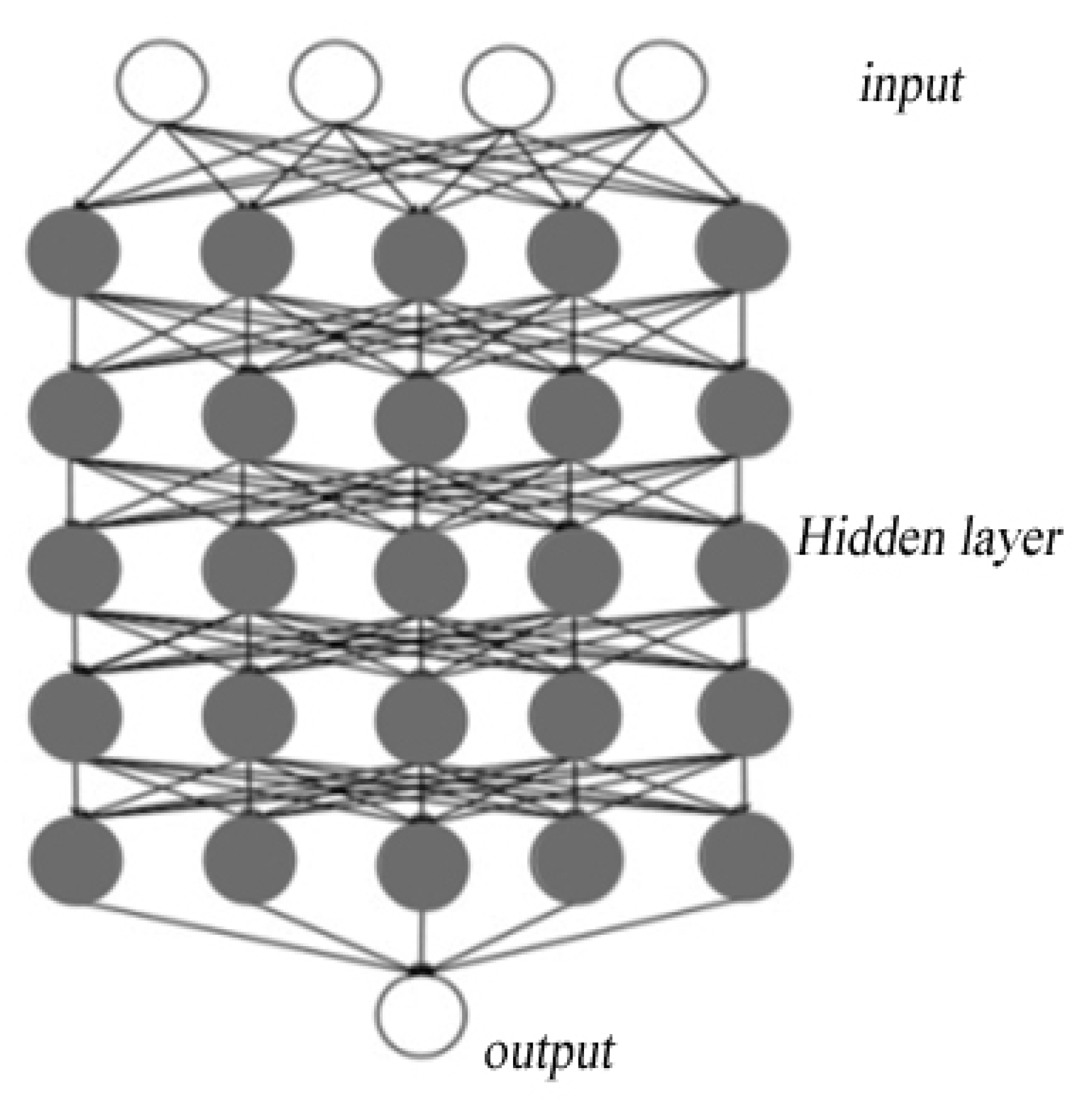
(1) Deep learning has a more complex structure than shallow learning does. It improves the ability of the model to learn complex, non-linear functions by increasing its depth. In general, the deep learning model can have more than 10 hidden layers. The structures of shallow learning and deep learning are shown in Figure 1 and Figure 2, respectively.
(2) Deep learning has a better learning ability than shallow learning does, such that it can provide a more comprehensive description of the characteristics of and relationships among the data. This, in turn, improves the capability of the model to learn better features and, thus, improve its predictive accuracy.
There are many methods of deep learning. We used the depth-based belief neural network (DBNN), which is widely used for character recognition [24], and the deep convolutional neural network (DCNN) [25,26], which is widely used in image recognition, to establish a surrogate model of the simulation model.
We give examples of these two methods below. The first involves constructing a surrogate model by using the DBNN:
(1)
Normalizing the target:
x i = x i x min x max x min
where x i represents the original values of the data, x min represents their minimum values, x max denotes their maximum values, and x i are their normalized values, x i [ 0 , 1 ] . The normalized x i values are used to construct the surrogate model.
(2)
Using DBNN to replace the setting of the model parameters:
Parameter Initialization
Based on past experience, the initial values of the weights and thresholds were set to w = 0 , a = 0 , and b = 0 . The learning rate reflects the speed of the parameter update and its value influences the speed of the training of the network and the accuracy of the simulation of the model. Too high a learning speed can cause the reconstruction error to grow easily and very quickly, such that the DBNN cannot converge or becomes unstable. This leads to a decline in its capability to perform feature extraction. If the learning rate is too low, overfitting occurs which reduces the speed of the update of the parameters and increases the training time of the model [27].
  • Numbers of Hidden Layers
The DBNN model is generally composed of a multi-layered RBM and a neural network (the BP neural network is the most commonly used one) [28]. As the number of layers of the RBM increases, the accuracy of the feature extraction of the model increases. On the contrary, the training time also increases which enhances the loss of information, which affects the accuracy of the model. It is therefore important to select the optimal number of layers according to the given situation to optimize the results that are to be produced. The BP neural network that is used in this study applied a three-layer structure to output continuous predictions.
  • Determining the Number of odes in the Hidden Layers
The agent model is an important part of the overall model. The number of neuronal nodes in the visible layer of the network is usually taken as its input variable and the number of nodes in the output layer is taken as its output variable. During training, the number of neurons in the middle layer is determined by manual fine-tuning and empirical formulas. The calculation is as follows:
h = m + n + a , a [ 1 , 10 ]
h = m n + k 2 , k [ 1 , 10 ]
h = m n + n
where m stands for the number of nodes of the input layer and n is the number of nodes of the output layer.
(3)
Unsupervised learning:
Based on the previous step, the RBM is trained with sample data. The first layer is used to obtain the characteristics of the sample data which are then used as the input for the next layer. These steps are repeated to train all of the RBMs. Following this, the feature vector of the training samples is outputted as the input to the BP neural network for prediction and the trend of the reconstruction error is generated.
(4)
Fine-tuning the learning process:
The last step in constructing the DBNN model is supervised learning. This involves back-propagating the error to fine-tune each node of the network and enable it to converge to the global optimum to ensure the accuracy of the fitting of the data. The resulting DBNN model can be used for simulation and prediction.
(5)
Reverse data normalization:
x i = x i ( x max x min ) + x min
The parameters that are here are the same as in Equation (1).
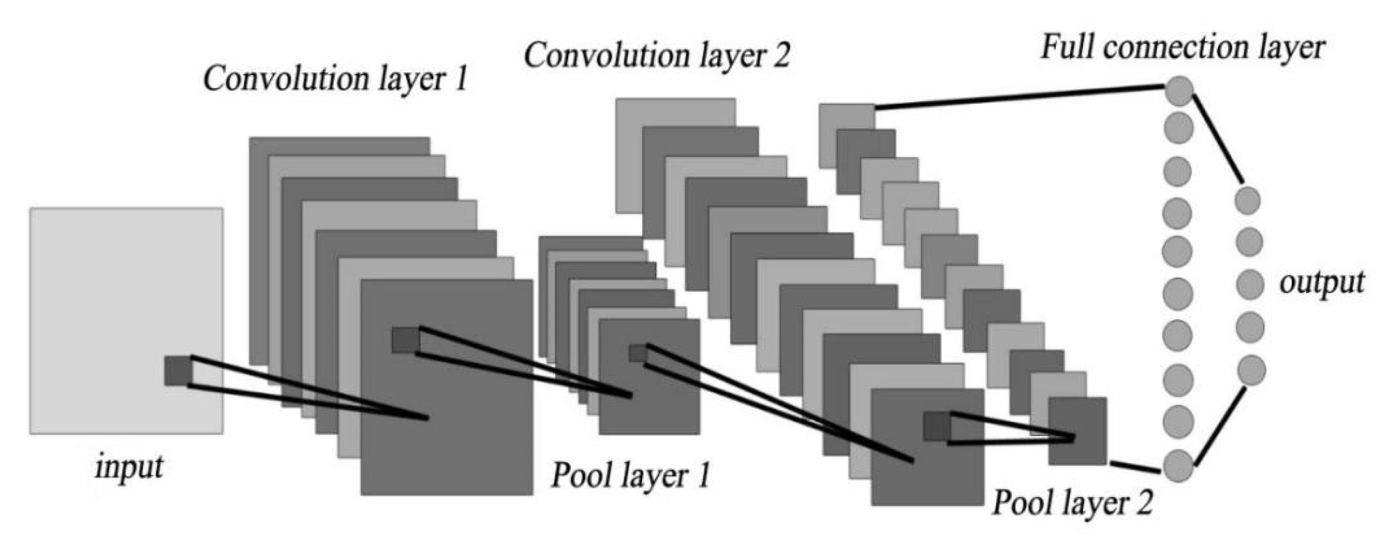
The DCNN is now introduced. It is a CNN with multiple hidden layers [29]. The network is mainly composed of a convolution layer, a pooling layer, and a fully connected layer as shown in Figure 3. It is essentially a multi-layer perceptron. Weight sharing and local connections are used in it to reduce the number of weights and make the network easy to optimize while reducing the risk of overfitting.
The sample data are first normalized, and the DCNN model is then trained and validated by using them in MATLAB. The surrogate model for the DCNN is finally established. The procedure is given below [30].
(1)
Principle of forward conduction:
Convolution layer: The local area of the input variables is convoluted by the convolution core in the convolution layer to generate the corresponding characteristic data, reduce the number of parameters of the convolution layer, and realize weight sharing. Weight sharing involves traversing the same convolution core once, in a fixed step, to reduce the memory that is required by the system and to avoid the overfitting that is caused by the use of too many parameters. It is the most important feature of the convolution layer. The formula is as follows:
y l ( i , j ) = K i l x l ( r j ) = j = 0 W 1 K i l ( j ) x l ( j + j )
In Formula (6), the l weight of the i convolution core at level j is recorded as K i l ( j ) , the local area j that is convoluted is recorded as x l ( r j ) , and the width of the convolution core is W . A diagram for the calculation of the convolution layer is given below.
Activation layer: The abovementioned output is used in the activation layer to map the original, linear, non-separable, and multi-dimensional features into another space by using an activation function. This enhances the linear separability of the features so that a non-linear transformation can be applied. The sigmoid function, hyperbolic tangent function tanh, and modified ReLU are common activation functions. They are expressed as follows:
a l ( i , j ) = S i g m o i d ( y l ( i , j ) ) = 1 1 + e y l ( i , j )
a l ( i , j ) = T a n h ( y l ( i , j ) ) = e y l ( i , j ) e y l ( i , j ) e y l ( i , j ) + e y l ( i , j )
a l ( i , j ) = f ( y l ( i , j ) ) = max { 0 , y l ( i , j ) }
In Formulas (7)–(9), the record of the output of the volume base is y l ( i , j ) and a l ( i , j ) is the activation value of y l ( i , j ) .
The sigmoid and tanh functions are used to update the weights by inverse error propagation, such that, as the number of layers of the network increases, the values of the sigmoid and tanh functions approach zero when the absolute value of the input is large, and the error cannot be propagated downward. This leads to a gradient dispersion. However, when the input to the ReLU function is greater than zero, the derivative is always one so that it avoids a gradient dispersion. Therefore, we used the ReLU function as the activation function for establishing the surrogate model of the DCNN.
Pooling layer: The pooling layer is located behind the convolution layer and is also known as the lower sampling layer. It forms a convolution–pooling unit together with the convolution layer. Its function is to extract the complete characteristics of the data. The pooling layer reduces the number of parameters of the DCNN through the use of pooling calculations. The structure of calculation of the convolution layer is shown in Figure 4.
Commonly used pooling functions include mean pooling and maximum pooling, and their mathematical descriptions are shown in Equations (10) and (11), respectively. The neurons in the perceptual domain are then calculated. The process is called maximum pooling when their maximum values are taken as the output, and it is called mean pooling their mean values are taken as the output.
p l ( i , j ) = 1 W t = ( j 1 ) W + 1 j W a l ( i , t )
p l ( i , j ) = max ( j 1 ) W + 1 t j W { a l ( i , t ) }
In the abovementioned calculation, the activation value of the t -th neuron in layer l and frame i is recorded as a l ( i , t ) . The width of the pooling area is W .
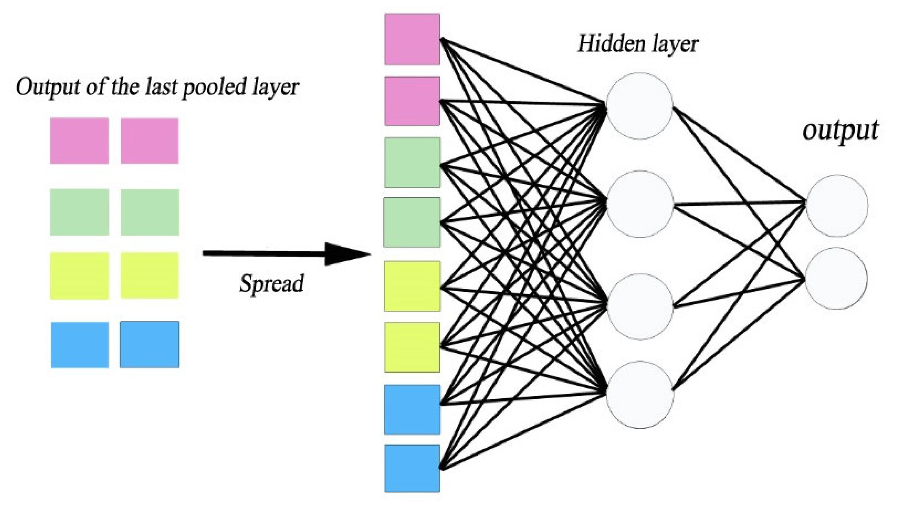
Fully connected layer: As shown in Figure 5, the inputs and outputs of this layer are fully connected. The input is a one-dimensional feature vector that is obtained from the output of the last pooling layer. The calculation is as follows:
z l + 1 ( j ) = i = 1 n W i j l a l ( i ) + b j l
In the abovementioned calculation, W i j l represents the weight between the i -th neuron in layer l and the j -th neuron in layer l + 1 , z l + 1 ( j ) is the value of the j -th output neuron at the l + 1 level, and b j l is the bias value of all of the neurons in layer l with respect to the j -th neuron in layer l + 1 .
Loss function: The loss function is used to evaluate the consistency of the output of the DCNN with respect to the corresponding target value. The commonly used loss function is the square error function. Assuming that the output of the DCNN is p and the target value is q, the mean error is as follows:
L = 1 m k = 1 m 1 2 ( p k q k ) 2
(2)
Principle of back-propagation:
The key step to optimize the weights of the DCNN is error back-propagation. It begins with the fully connected layer and gradually solves the derivatives of each layer. According to the chain rule, the derivative of the loss function with respect to the last neuron in the layer is the first one to be solved, and the calculation then is carried out in a step-by-step manner from back to front. It includes reverse derivations of the fully connected layer, pooling layer, and convolution layer, and the update of the weights. If the error is too large, errors in the upper layers can be calculated by a gradient descent according to the error in the output layer until the input layer is reached while the weights and offsets are continuously adjusted. The process is repeated until the accuracy-related requirements are met. This part is similar to reverse correction, and its description is not repeated here.

4. Establishing a Seawater Intrusion Simulation Model

Global climate change influences temperature, precipitation, and the sea level, and thus, it has an impact on hydrological forecasting. These factors directly affect the equilibrium between seawater and groundwater in aquifers in coastal areas. The uncertainty in the rise in sea level significantly affects the predictions of the model. We propose a 3D model for the numerical simulation and prediction of seawater intrusion. This will help to lay the foundation for the analysis of uncertainty in the rise in sea levels [31].
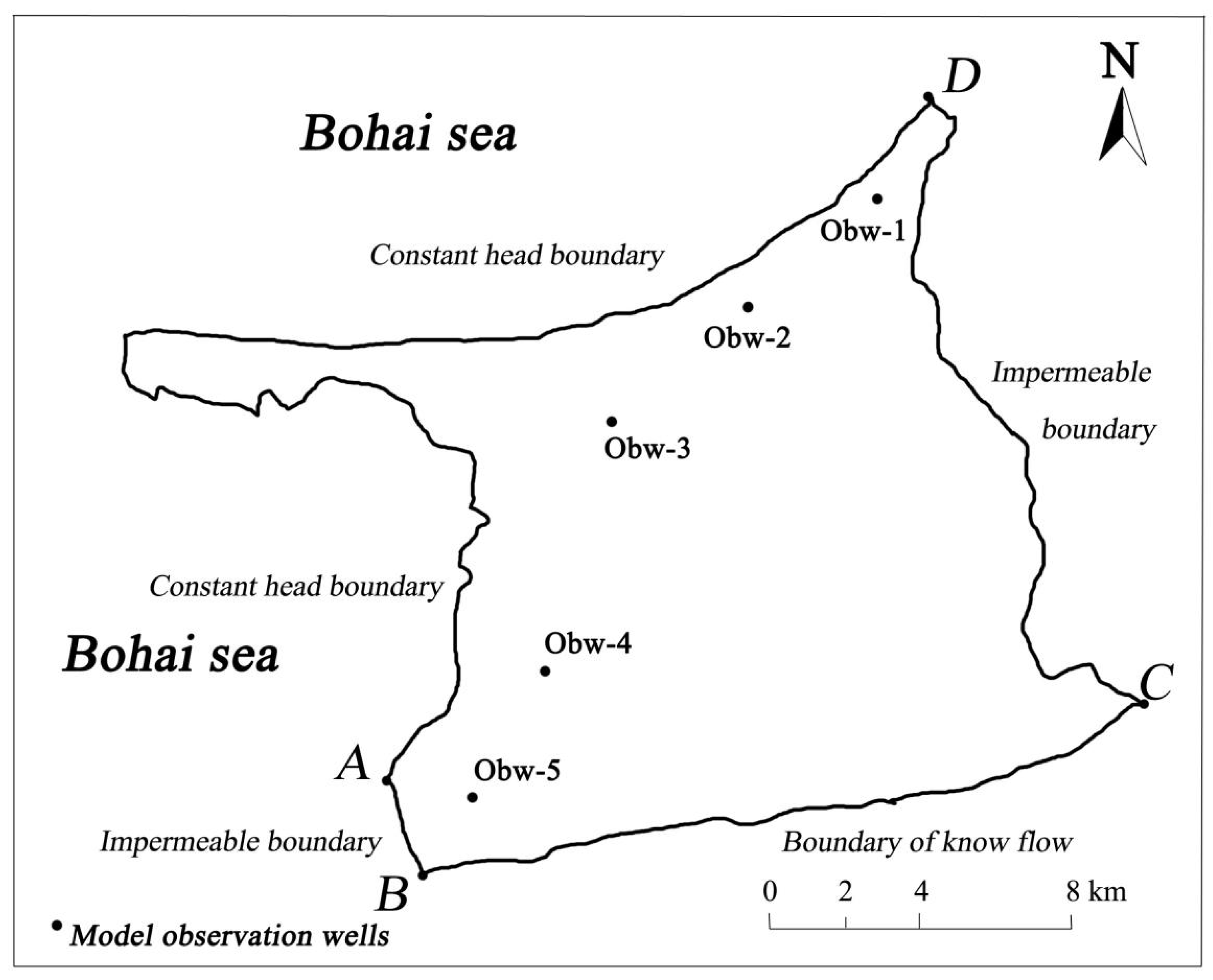
The area that was chosen for this study is Longkou City. It is located on the Jiaodong Peninsula in the Shandong Province of China. The maximum horizontal distance between the eastern and western boundaries of Longkou City is 46.08 km, the maximum vertical distance between its northern and southern boundaries is 37.43 km (Figure 6), the length of its coastal curve is 68.41 km, and its total area is 901 km2.
Longkou is adjacent to the Bohai Sea to the west and the north, and there are mountains, plateaus, and piedmont plains to its southeast. The terrain is high in the southeast and it is low in the northwest. The trend of the mountain ranges is north-to-east or north-to-south, and they gradually flatten to the north. The area is evenly divided between hills and plains in the mountainous areas. It has a warm and temperate monsoon climate with an average annual precipitation of 595 mm. The inter-annual variation in precipitation is large and its annual distribution is uneven under the influence of the monsoon. The annual average evaporation ranges from 1150 to 1250 mm, with higher evaporation in areas that are close to Beibu Gulf. The rivers in the study area run vertically and horizontally but they are not large, and most of them are seasonal. The main perennial river is Yongwen River.
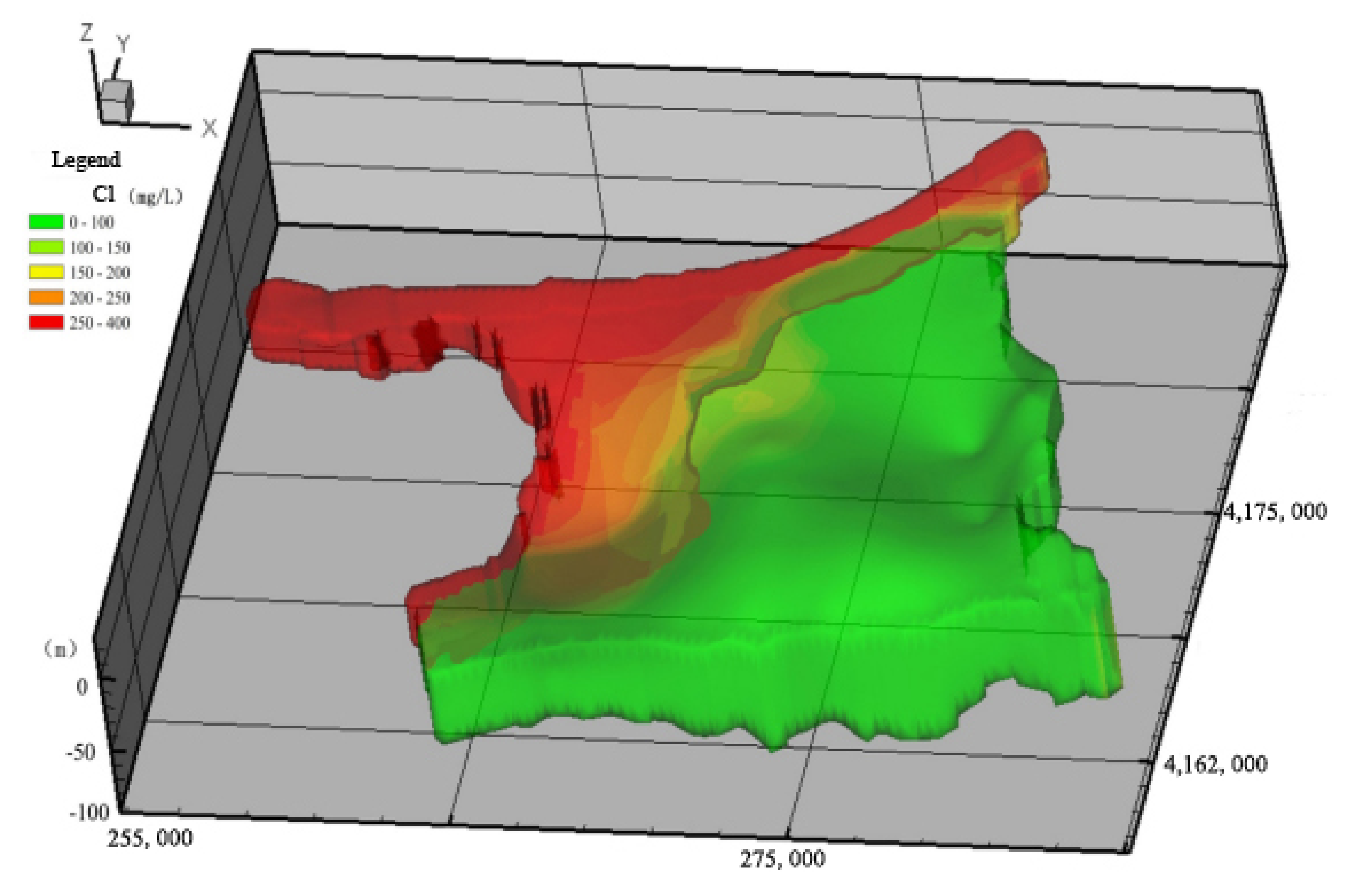
We collected the meteorological, hydrological, and geological data for the study area to establish a simulation model to describe seawater intrusion. According to the hydrogeological conditions of the study area, it can be generalized as a three-dimensional, heterogeneous, and isotropic porous water-bearing medium. The monthly precipitation infiltration is 16 million m3 per year, and the evaporation is about 1200 mm per year. The model consisted of models of flow and water quality [32]). It included partial differential equations and definite solution conditions, where the two were coupled based on the equations of motion. The model was solved by the SEAWAT program [33]. The measured data were substituted into the model for calculation, and the combination of the parameters was adjusted to satisfy the accuracy-related requirements. The inputs for the model included the sea level and the intensity of exploitation of groundwater, and the outputs consisted of the area of seawater intrusion and the Cl concentration in the typical observation wells. The concentrations of Cl in five observation wells and the area of seawater intrusion (Cl > 250 mg/L) in the study area were selected as the outputs to analyze the impact of uncertainty in the rise in sea levels on seawater intrusion. Figure 7 shows the results of the model.

5. Establishment of the Surrogate Model

The inputs for the model were determined according to the needs of research [34]. They included the pumping capacity and the rise in seawater levels in the group of wells in the study area. The inputs and outputs were substituted into the simulation model, and the corresponding output was calculated as the training sample.
Given that we sought to assess the influence of uncertainty in the rise in sea levels on the results of the simulations, we took this as a random variable. The range of the values of the random variable was set to a normal distribution according to authoritative research on China (80–170 mm). Latin hypercube sampling was used to ensure the representativeness of the sampling. The volume of the mining of the wells was their current pumping volume (see Table 1 for details). The other parameters of the models were consistent with the previous corrections.
According to the abovementioned parameters, 100 groups of training samples were calculated to train the model, and another 20 groups of data were calculated as validation samples to test the accuracy of the surrogate model. We used the DBNN, radial basis function (RBF) [35,36], a typical neural network, and the DCNN to establish surrogate models of seawater intrusion. The 20 groups of the validation samples were used to check the accuracy of the models.
The degrees of approximation of these surrogate models to the simulation model were analyzed and compared, and the most accurate one was selected for subsequent research [37]. We also evaluated the accuracy of the surrogate models by using four indices to assess their precision, and the results are shown in Table 2.
Of the surrogate models, the output of the one for the DBNN was closest to that of the analog model. Table 2 shows that it was superior to the other methods on the three indices of the maximum relative error, average relative error, and root mean-squared error, with values of 3.961%, 1.658%, and 3.707, respectively. The closer that the coefficient of determination of accuracy was to one, then the higher the accuracy was. The DBNN was 0.989, which is better than other methods (close to 1). It can, thus, be concluded that the DBNN was the most suitable for simulating the variable density of groundwater flow in the study area.
The DBNN method reduces the dependence of the accuracy of the model on the number of training samples by superimposing the RBM and using unsupervised learning. In addition, the increase in the number of layers of the model helps to improve its ability to represent complex non-linear functions and feature learning. The surrogate model of the DCNN, although more precise, is more heavily dependent on the size of the sample data, has a better learning ability for a large number of samples, and is suitable for a more diverse range of input–output combinations.
We thus applied the theory and method of the DBNN to map the relationship between the inputs and outputs to solve the model for seawater intrusion in the presence of a few training samples.
We used the Monte Carlo method to analyze the impact of randomness in the rise in sea levels. The model needs to be called repeatedly in the simulation [38]. This incurs a large burden of calculation and takes a long time, which is not conducive to its use in applications. A surrogate model is an approximation of the analog model that can reduce the calculation load and the time that is needed to perform its function, while guaranteeing high accuracy. We thus used the DBNN model that was established in a previous paper [39] instead of the simulation model for the Monte Carlo simulation.

6. Results and Discussion

We set up a simulation model to describe the study area. In light of the uncertain impact of global climate change on the rise in sea level, we took the sea level as a random variable, established a surrogate model for the simulation model by using the DBNN, and conducted an uncertainty analysis based on it by using the Monte Carlo method. The processor that was used for the simulations was an i7-4790k (4 GHz), with 16 GB of memory and a Windows 7 operating system (×64). We ran GMS 10.0 to solve the model, and this took about 370 s. If the simulation model was directly used for uncertainty analysis, it needed to be calculated 200 times, which required 20.5 h. The surrogate model was used in place of the simulation model for uncertainty analysis. The simulation model needed to be run 120 times to establish the surrogate, which took 12.3 h. Calling the surrogate model in the Monte Carlo simulation took only 5 s, thus reducing the time that was needed for calculation by 40%. As the number of random tests was increased, more calculation time was saved.
The rise in sea level was taken as a random variable, and 200 sets of samples were taken from the range of this variable by employing Latin hypercube sampling [40,41] as the input to the surrogate model, while the other input variables (the pumping capacity of the three well groups) were treated as deterministic values according to the current production volumes (the random range of rise in sea levels was predicted by an atmospheric circulation model.) The results of the sampling of the random variables were inputted into the DBNN surrogate model, and the concentrations of Cl and areas of seawater intrusion in the five observation wells were calculated. The outputs (Cl−concentration) of each well were then statistically analyzed.
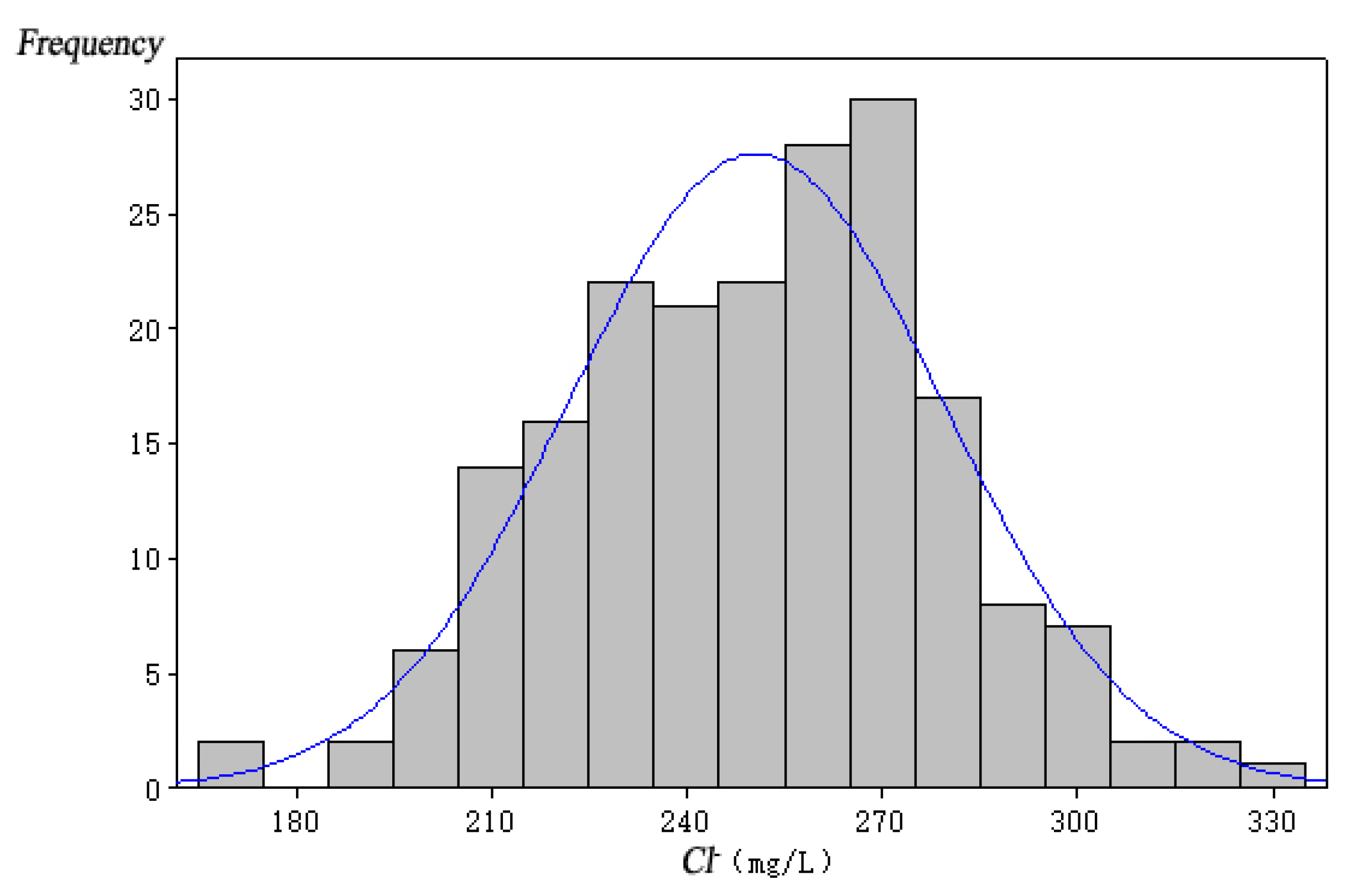
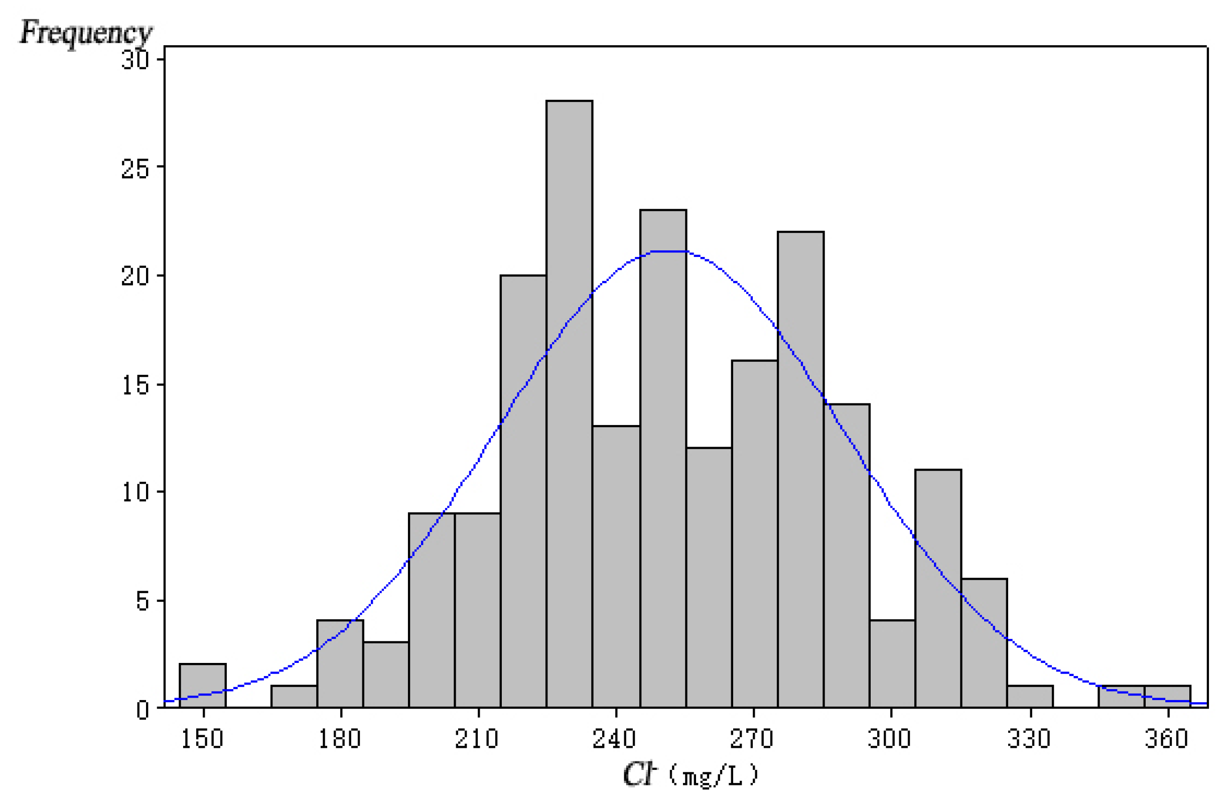
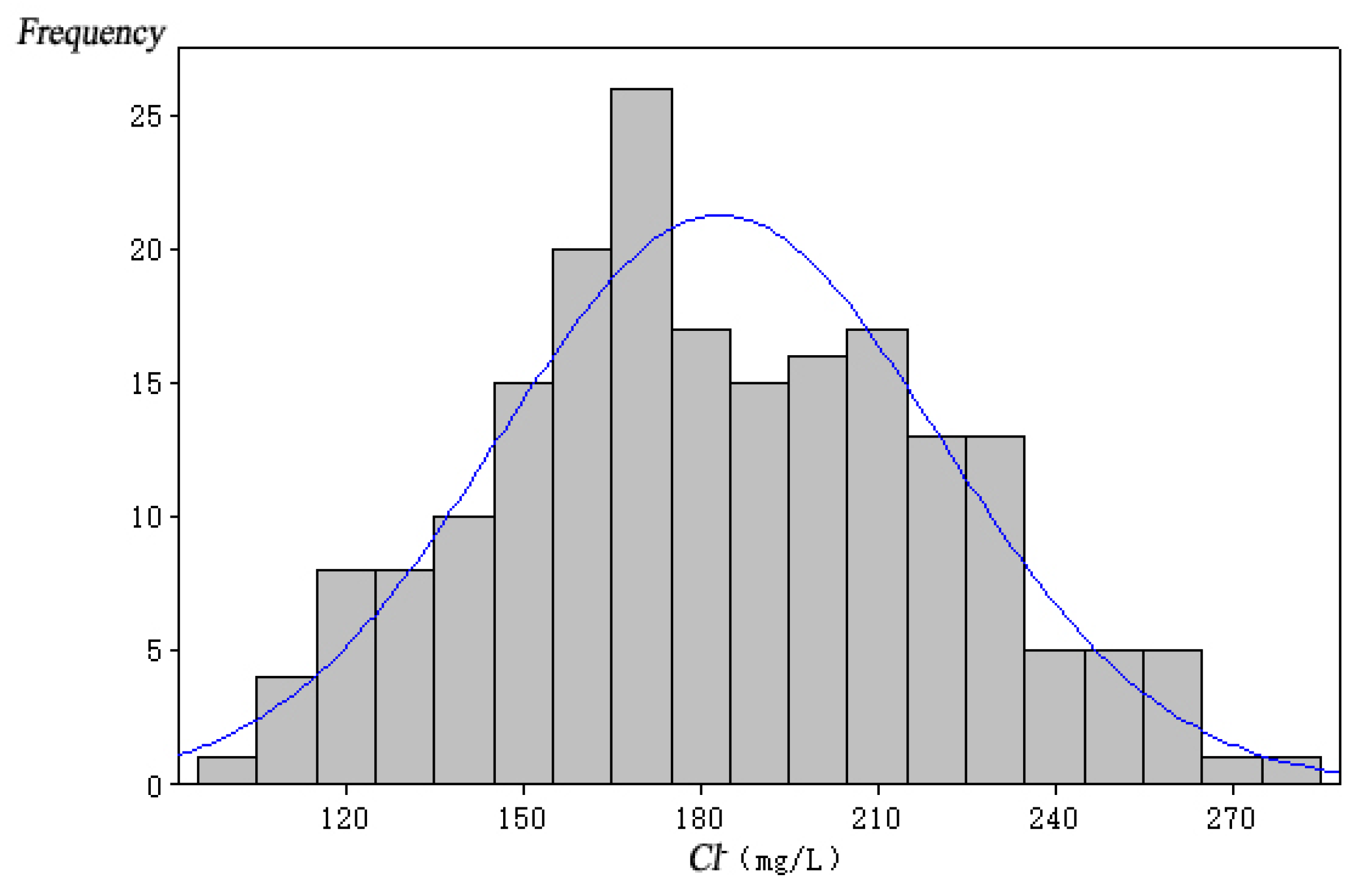
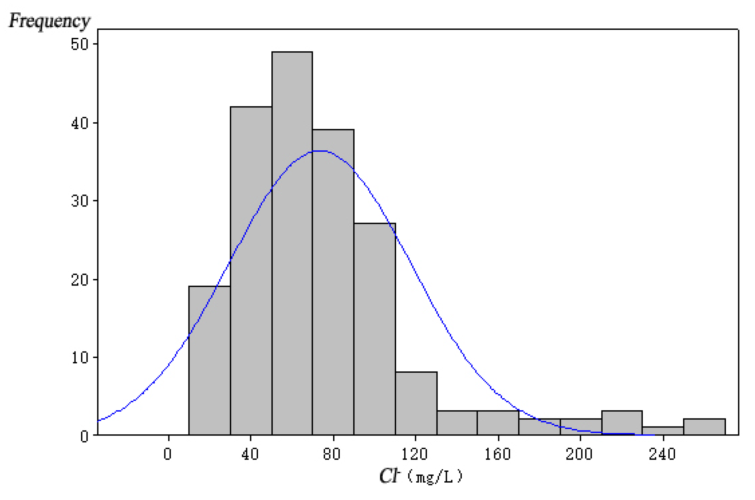
Histograms of the chloride concentration in each observation well (ObW) are shown in Figure 8, Figure 9, Figure 10, Figure 11 and Figure 12. The statistical indicators are shown in Table 3.
A comparison of Figure 8 and Figure 10 shows that both of the wells ObW-1 and ObW-3 had more frequent occurrences of chloride ion concentrations that were greater than 250 mg/L at the end of the simulation period, which indicates that these two wells were more prone to seawater intrusion than the others were. Figure 11 and Figure 12 show that the chloride concentrations of the wells ObW-4 and ObW-5 at the end of the simulation period were below 200 mg/L, which indicates that these wells were not susceptible to seawater intrusion. The concentration of chloride ion in ObW-5 was below 100 mg/L, and thus it was the least susceptible to seawater intrusion.
In Table 3, the standard deviation reflects the degree of data dispersion. The larger the standard deviation is, the more scattered the outputs are, thus indicating a greater uncertainty. Due to the randomness of the rise in sea levels, the chloride ion concentration of each well fluctuated. The standard deviation also reflected the sensitivity of each well to the rise in sea level. The output of ObW-1 was the least discrete, while that of ObW-3 was the most discrete, which indicates that the latter was most affected by the randomness of the rise in sea levels. ObW-5 was, thus, the least susceptible to seawater intrusion and ObW-3 was at the greatest risk.
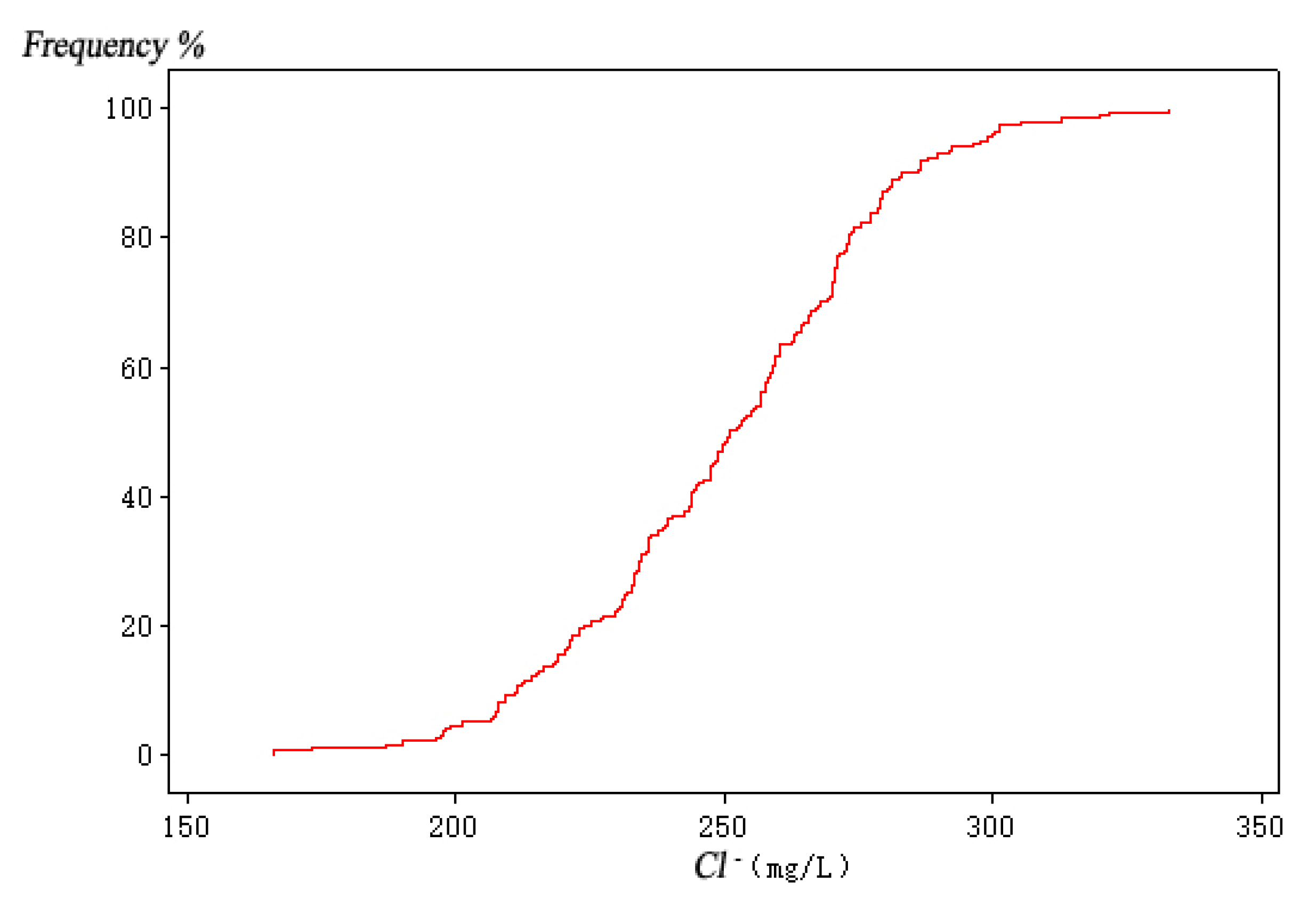
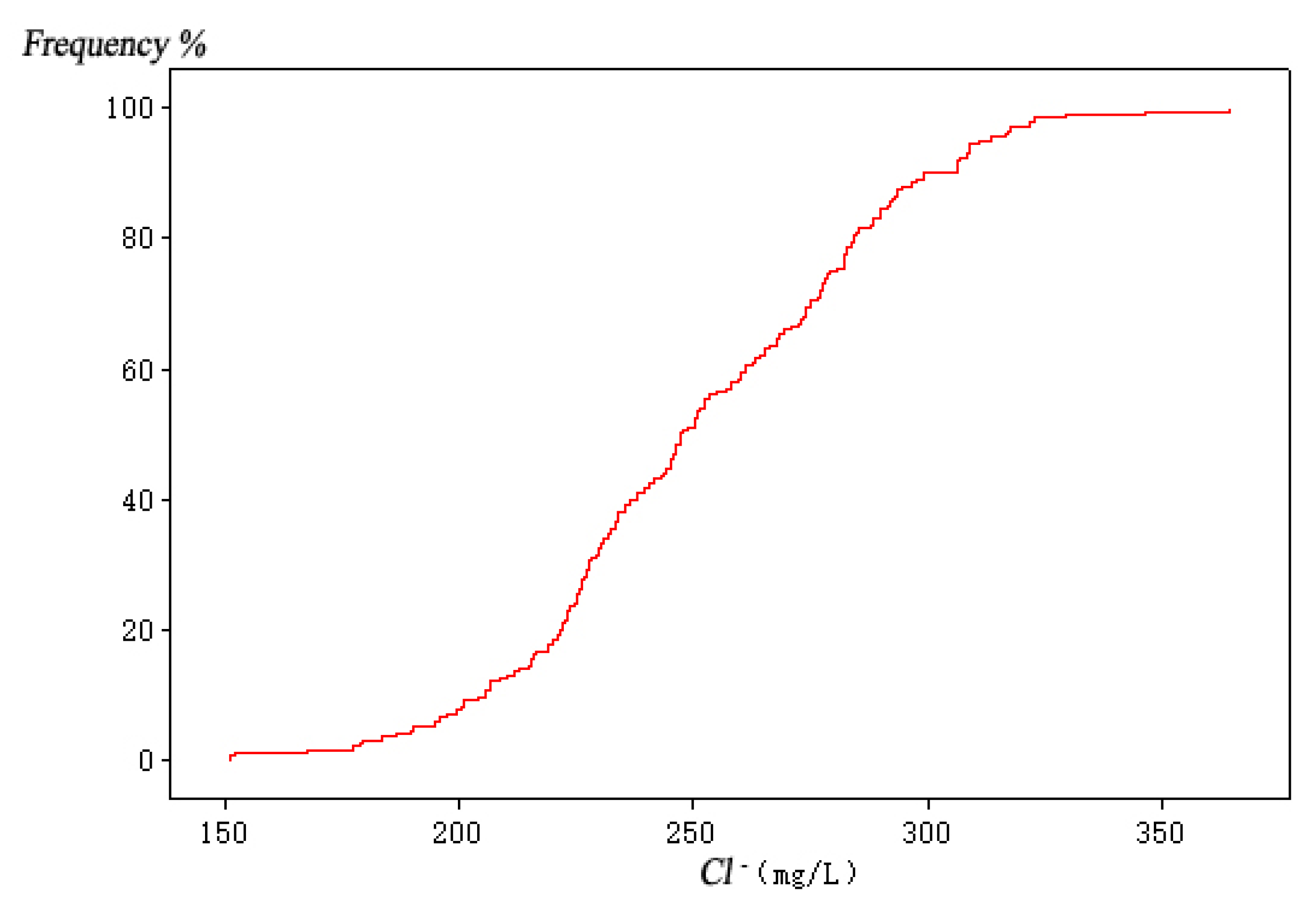
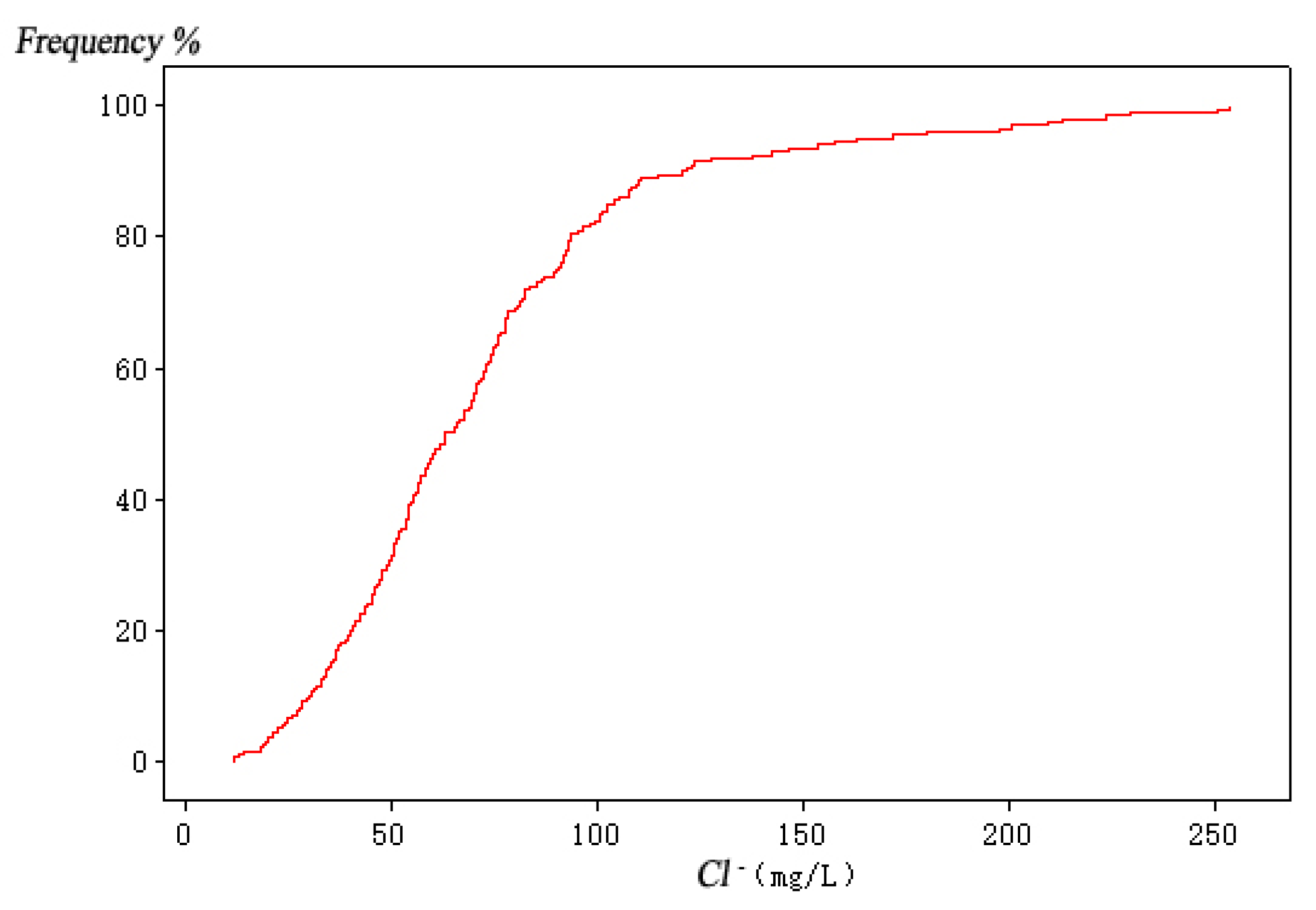
The risk of seawater intrusion in each well was then assessed. The curve of the cumulative distribution of the probability of seawater intrusion for each well is plotted as shown in Figure 13, Figure 14, Figure 15, Figure 16 and Figure 17. The risk of seawater intrusion of each well is shown in Table 4.
Figure 13, Figure 14, Figure 15, Figure 16 and Figure 17 and Table 4 show that the probability of seawater intrusion in ObW-3 was 58%, while that in ObW-5 was only 1%. This result might have been obtained because the western aquifer in the study area where ObW-5 was located was thick, and it was not significantly affected by the randomness of the rise in sea level. However, ObW-3 well is located at the center of Longkou, near the Longkou Coal Mine, and its aquifer is thin, such that, it is susceptible to the randomness of the rise in sea level. Pressure mining and the construction of a cut-off wall near ObW-3 should be prioritized to prevent further impact on the activities of production and life by seawater intrusion.
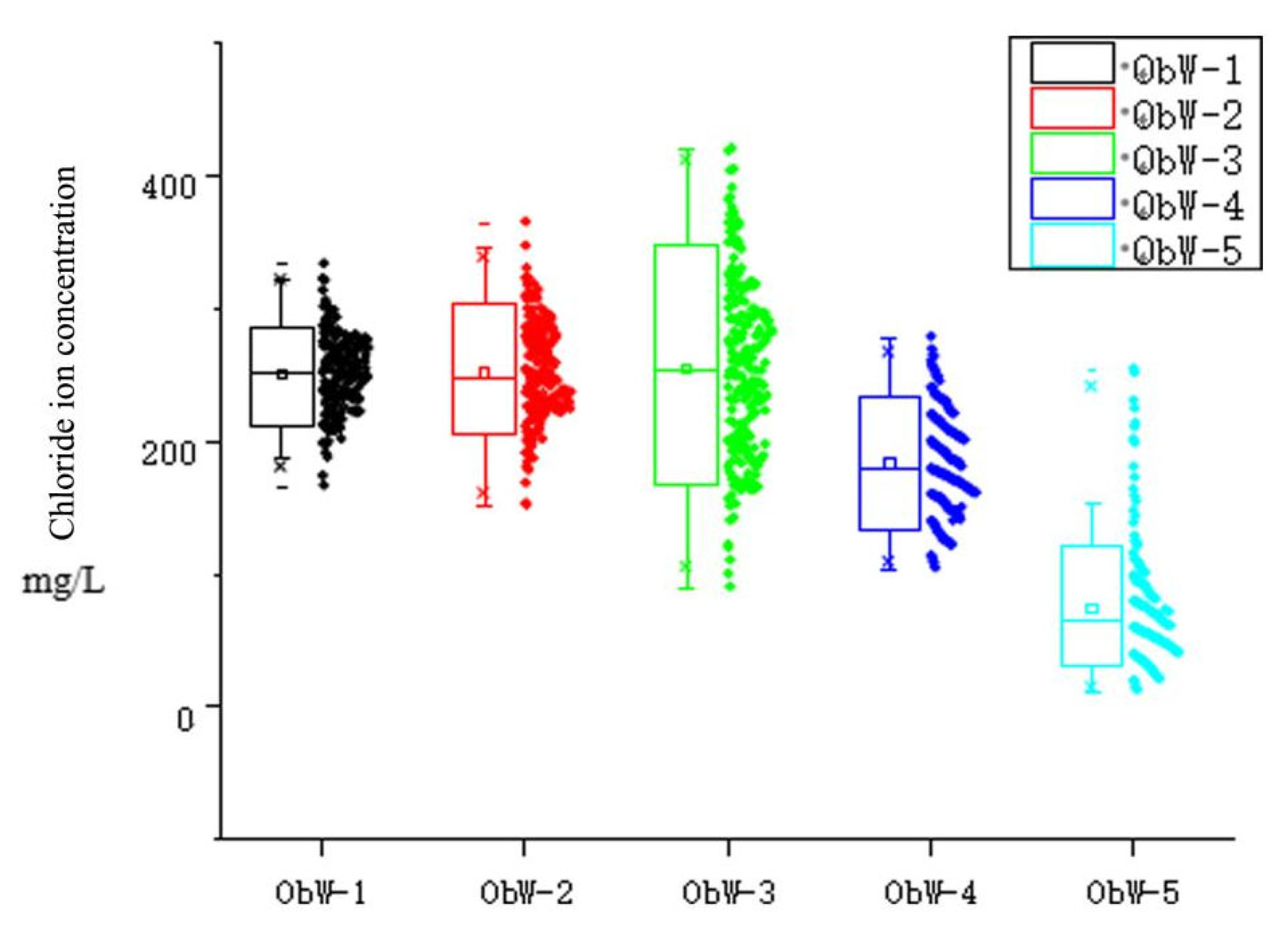
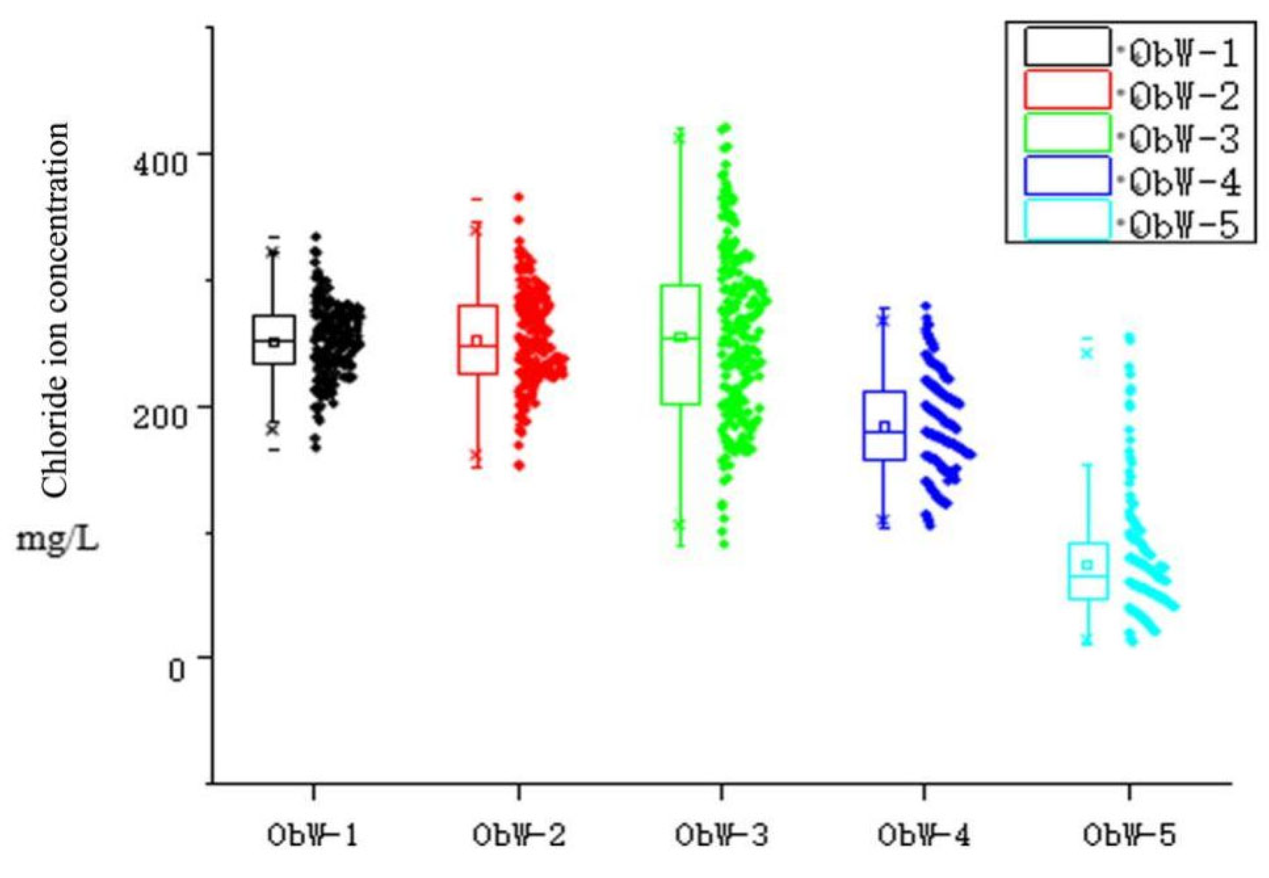
The confidence intervals of chloride ion concentrations in each well that were at confidence levels of 50% and 80% were also calculated. The higher the confidence level was, then the wider the range of the interval and the higher the probability of the data falling in the interval were. Chloride ion concentrations in the wells with these levels of confidence are plotted in Figure 18 and Figure 19, and the relevant statistics are detailed in Table 5.
Figure 18 and Figure 19 and Table 5 show that for the same confidence level, the confidence interval of well Obw-3 was the largest of all of the wells that were considered. When the confidence level was 80%, the confidence interval was 167.26–346.96 mg/L, indicating that this well was the most vulnerable to uncertainty in the sea level. The reliability of predictions for this well was poor when the deterministic model was used. The confidence interval of Obw-1 was the smallest. When the deterministic model was used to make predictions, the predicted chloride ion concentrations were the most reliable.
Finally, we statistically analyzed the area of the seawater intrusion, and the results are summarized in Table 6.
According to Table 6, the average area of the seawater intrusion at the end of the simulation period was 69.39 km2, which was close to the result that was predicted by the deterministic model (68.5 km2). The standard deviation of the area of the seawater intrusion was 7.31 km2, which was lower than the standard deviation of the chloride ion concentration in each well. This indicated that the randomness of the rise in sea level had a smaller impact on the area of the seawater intrusion in the study area than it did on the chloride ion concentration in the wells in the area.
To sum this up, the uncertainty analysis comprehensively reflects the relationship between the uncertain impact of global climate change on the rise in sea level and seawater intrusion. It thus provides strong support for guiding measures for extracting groundwater and protecting the research area.

7. Conclusions

In light of the uncertain impact of climate change on the sea level, this study used the rise in sea level as a random variable to determine the influence of the randomness in it on uncertainty in its simulation and prediction, and we applied the Monte Carlo method to conduct an uncertainty analysis. The results of the study adequately reflected the actual situation in the study area, which is expected to exhibit a complicated response to seawater intrusion. The results that are here can provide a reference for optimizing the exploitation of groundwater and can provide a basis for research on the prevention and control of seawater intrusion by using AI-based methods. In addition, the results showed that using the surrogate model instead of the simulation model for this calculation when also using the Monte Carlo method for uncertainty analysis could ensure highly accurate results while significantly reducing the calculation time.

Author Contributions

Conceptualization, T.M. and J.G.; software, H.H. and Y.Z.; resources, N.C.; data curation, G.L.; writing—original draft preparation, T.M.; writing—review and editing, J.G. All authors have read and agreed to the published version of the manuscript.

Funding

This research received no external funding.

Data Availability Statement

The data presented in this study are available on request from the corresponding.

Conflicts of Interest

The authors declare no conflict of interest. The funders had no role in the design of the study; in the collection, analyses, or interpretation of data; in the writing of the manuscript, or in the decision to publish the results.

References

  1. Lin, J.; Snodsmith, J.B.; Zheng, C.; Wu, J. A modeling study of seawater intrusion in Alabama Gulf Coast, USA. Environ. Geol. 2009, 57, 119–130. [Google Scholar] [CrossRef]
  2. Kaleris, Vassilios K.;Ziogas, Alexandros I..Using electrical resistivity logs and short duration pumping tests to estimate hydraulic conductivity profiles. J. Hydrol. 2020, 590, 125277. [CrossRef]
  3. Ketabchi, H.; Mahmoodzadeh, D.; Ataie-Ashtiani, B.; Simmons, C.T. Sea-level rise impacts on seawater intrusion in coastal aquifers: Review and integration. J. Hydrol. 2016, 535, 235–255. [Google Scholar] [CrossRef]
  4. Larsen, F.; Tran, L.V.; Van Hoang, H.; Tran, L.T.; Christiansen, A.V.; Pham, N.Q. Groundwater salinity influe.nced by Holocene seawater trapped in incised valleys in the Red River delta plain. Nat. Geosci. 2017, 10, 376–381. [Google Scholar] [CrossRef]
  5. Fan, Y.; Lu, W.; Miao, T.; Li, J.; Lin, J. Multiobjective optimization of the groundwater exploitation layout in coastal areas based on multiple surrogate models. Environ. Sci. Pollut. Res. 2020, 27, 19561–19576. [Google Scholar] [CrossRef]
  6. El Bilali, A.; Taleb, A.; Brouziyne, Y. Comparing four machine learning model performances in forecasting the alluvial aquifer level in a semi-arid region. J. Afr. Earth Sci. 2021, 181, 104244. [Google Scholar] [CrossRef]
  7. Miao, T.; Lu, W.; Lin, J.; Guo, J.; Liu, T. Modeling and uncertainty analysis of seawater intrusion in coastal aquifers using a surrogate model: A case study in Longkou, China. Arab. J. Geosci. 2019, 12, 1. [Google Scholar] [CrossRef]
  8. Singh, A.; Hauffpauir, R.; Mishra, S.; Lavenue, M.; Valocchi, A. Analyzing Uncertainty and Risk in the Management of Water Resources for the Texas Water Development Board. In Proceedings of the World Environmental & Water Resources Congress, Providence, RI, USA, 16–20 May 2010. [Google Scholar]
  9. Allgeier, J.; González-Nicolás, A.; Erdal, D.; Nowak, W.; Cirpka, O.A. A Stochastic Framework to Optimize Monitoring Strategies for Delineating Groundwater Divides. Front. Earth Sci. 2020, 8, 554845. [Google Scholar] [CrossRef]
  10. Gallagher, M.; Doherty, J. Parameter estimation and uncertainty analysis for a watershed model. Environ. Model. Softw. 2007, 22, 1000–1020. [Google Scholar] [CrossRef]
  11. Wu, J.C.; Lu, L.; Tang, T. Bayesian analysis for uncertainty and risk in a groundwater numerical model’s predictions. Hum. Ecol. Risk Assess. Int. J. 2011, 17, 1310–1331. [Google Scholar] [CrossRef]
  12. Neufeld, D.; Behdinan, K.; Chung, J. Aircraft wing box optimization considering uncertainty in surrogate models. Struct. Multidiscip. Optim. 2010, 42, 745–753. [Google Scholar] [CrossRef]
  13. Miao, T.S.; Lu, W.X.; Ouyang, Q. Application of Uncertainty Analysis of Groundwater Numerical Simulation in Water Quality Prediction. Water Resour. Power 2016, 34, 20–23. [Google Scholar]
  14. Koohbor, B.; Fahs, M.; Ataie-Ashtiani, B.; Belfort, B.; Simmons, C.T.; Younes, A. Uncertainty analysis for seawater intrusion in fractured coastal aquifers: Effects of fracture location, aperture, density and hydrodynamic parameters. J. Hydrol. 2019, 571, 159–177. [Google Scholar] [CrossRef]
  15. Abd-Elhamid, H.F.; Javadi, A.A. Impact of sea level rise and over-pumping on seawater intrusion in coastal aquifers. J. Water Clim. Chang. 2011, 2, 19. [Google Scholar] [CrossRef]
  16. Bohorquez, P.; Ancey, C. Stochastic-deterministic modeling of bed load transport in shallow water flow over erodible slope: Linear stability analysis and numerical simulation. Adv. Water Resour. 2015, 83, 36–54. [Google Scholar] [CrossRef]
  17. Lee, J.; Kang, S. GA based meta-modeling of BPN architecture for constrained approximate optimization. Int. J. Solids Struct. 2007, 44, 5980–5993. [Google Scholar] [CrossRef]
  18. Hou, Z.; Lu, W. Stochastic nonlinear programming based on uncertainty analysis for DNAPL-contaminated aquifer remediation strategy optimization. J. Water Resour. Plan. Manag. 2018, 144, 04017076. [Google Scholar] [CrossRef]
  19. Won, K.S.; Ray, T. A framework for design optimization using surrogates. Eng. Optim. 2005, 37, 685–703. [Google Scholar] [CrossRef]
  20. Sreekanth, J.; Datta, B. Multi-objective management of saltwater intrusion in coastal aquifers using genetic programming and modular neural network based surrogate models. J. Hydrol. 2010, 393, 245–256. [Google Scholar] [CrossRef]
  21. Bengio, Y.; Courville, A.; Vincent, P. Unsupervised Feature Learning and Deep Learning: A Review and New Perspectives. arXiv 2012, arXiv: 1206.5538. [Google Scholar]
  22. Goodfellow, I.; Bengio, Y.; Courville, A. Deep Learning; MIT Press: Cambridge, MA, USA, 2016. [Google Scholar]
  23. Li, Z.; Gong, B.; Yang, T. Improved Dropout for Shallow and Deep Learning. In Proceedings of the Advances in Neural Information Processing Systems 29: Annual Conference on Neural Information Processing Systems 2016, Barcelona, Spain, 5–10 December 2016. [Google Scholar]
  24. Luger, G. Artificial Intelligence: Structures and Strategies for Complex Problem Solving, 5th ed.; Pearson Addison Wesley: San Francisco, CA, USA, 2004. [Google Scholar]
  25. Xiao, T.; Xu, Y.; Yang, K.; Zhang, J.; Peng, Y.; Zhang, Z. The Application of Two-level Attention Models in Deep Convolutional Neural Network for Fine-grained Image Classification. In Proceedings of the Proceedings of the IEEE conference on computer vision and pattern recognition, Washington, DC, USA, 23–28 June 2014. [Google Scholar]
  26. Xu, L.; Ren, J.S.; Liu, C.; Jia, J. Deep Convolutional Neural Network for Image Deconvolution. In International Conference on Neural Information Processing Systems; MIT Press: Cambridge, MA, USA, 2014; pp. 1790–1798. [Google Scholar]
  27. Ferrag, M.A.; Maglaras, L.; Moschoyiannis, S.; Janicke, H. Deep learning for cyber security intrusion detection: Approaches, datasets, and comparative study. Inf. Secur. Technol. Rep. 2020, 50, 102419.1–102419.19. [Google Scholar] [CrossRef]
  28. Schölkopf, B.; Platt, J.; Hofmann, T. Greedy layer-wise training of deep networks. In Advances in Neural Information Processing Systems 19: Proceedings of the 2006 Conference; MIT Press: Cambridge, MA, USA, 2007. [Google Scholar]
  29. Hinton, G.E.; Osindero, S.; Teh, Y.W. A fast learning algorithm for deep belief nets. Neural Comput. 2006, 18, 1527–1554. [Google Scholar] [CrossRef] [PubMed]
  30. Vedaldi, A.; Lenc, K. MatConvNet—Convolutional Neural Networks for MATLAB. In Proceedings of the 23rd ACM International Conference, ACM, Brisbane, Australia, 26–30 October 2015. [Google Scholar]
  31. Allen, C.D.; Macalady, A.K.; Chenchouni, H.; Bachelet, D.; McDowell, N.; Vennetier, M.; Kitzberger, T.; Rigling, A.; Breshears, D.D.; Hogg, E.H. A global overview of drought and heat-induced tree mortality reveals emerging climate change risks for forests. For. Ecol. Manag. 2010, 259, 660–684. [Google Scholar] [CrossRef]
  32. Praveena, S.M.; Lin, C.Y.; Aris, A.Z.; Abdullah, M.H. Groundwater assessment at Manukan Island, Sabah: Multidisciplinary approaches. Nat. Resour. Res. 2010, 19, 279–291. [Google Scholar] [CrossRef]
  33. Langevin, C.D. SEAWAT: A Computer Program for Simulation of Variable-Density Groundwater Flow and Multi-Species Solute and Heat Transport; US Geological Survey: Menlo Park, CA, USA, 2009. [Google Scholar]
  34. Wagner, M.; Wilson, J.R. Using Univariate Bezier Distributions to Model Simulation Input Processes. A I I E Trans. 1994, 28, 699–711. [Google Scholar] [CrossRef]
  35. Park, J.; Sandberg, I. Universal Approximation Using Radial-Basis-Function Networks. Neural Comput. 2014, 3, 246–257. [Google Scholar] [CrossRef]
  36. Slpponen, P.; Kekki, M.; Haapakoski, J.; Ihamäki, T.; Siurala, M. Gastric cancer risk in chronic atrophic gastritis: Statistical calculations of cross-sectional data. Int. J. Cancer 1985, 35, 173–177. [Google Scholar] [CrossRef]
  37. Papadopoulos, C.E.; Yeung, H. Uncertainty estimation and Monte Carlo simulation method. Flow Meas. Instrum. 2002, 12, 291–298. [Google Scholar] [CrossRef]
  38. Lo, S.C.; Ma, H.W.; Lo, S.L. Quantifying and reducing uncertainty in life cycle assessment using the Bayesian Monte Carlo method. Sci. Total Environ. 2005, 340, 23–33. [Google Scholar] [CrossRef]
  39. Miao, T.; Guo, J. Application of artificial intelligence deep learning in numerical simulation of seawater intrusion. Environ. Sci. Pollut. Res. 2021, 28, 54096–54104. [Google Scholar] [CrossRef]
  40. Olsson, A.; Sandberg, G.; Dahlblom, O. On Latin hypercube sampling for structural reliability analysis. Struct. Saf. 2003, 25, 47–68. [Google Scholar] [CrossRef]
  41. Iman, R.L. Latin Hypercube Sampling; American Cancer Society: Atlanta, GA, USA, 2008. [Google Scholar]
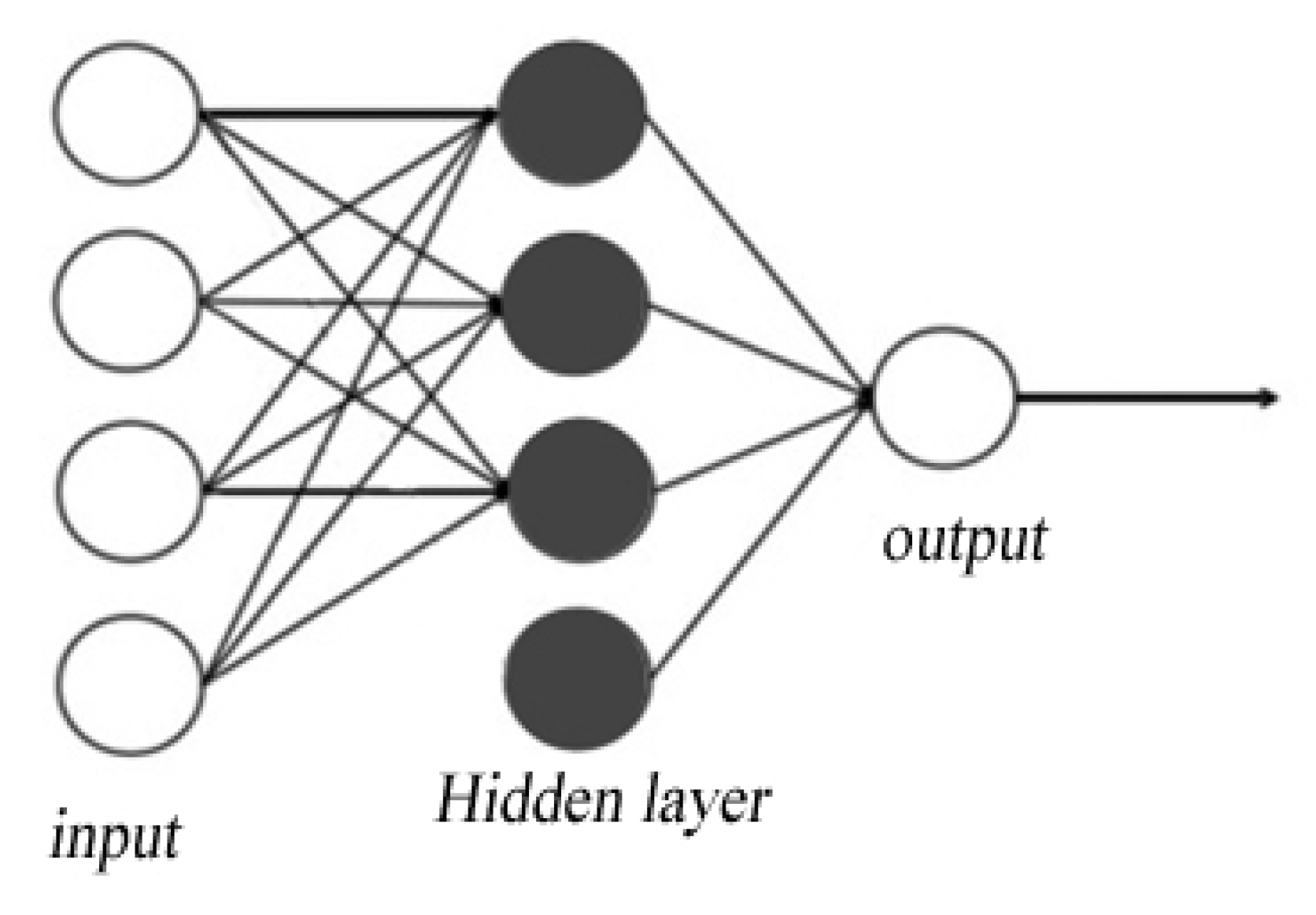
Figure 1. Logic diagram of shallow learning.
Water 14 02933 g001
Figure 2. Structural diagram of deep learning.
Water 14 02933 g002
Figure 3. Structure of the DCNN.
Water 14 02933 g003
Figure 4. Diagram of the calculation of the convolution layer.
Water 14 02933 g004
Figure 5. Fully connected layer.
Water 14 02933 g005
Figure 6. The boundary of the study and the observation wells that are in it (model output).
Water 14 02933 g006
Figure 7. Results of calculation of the model.
Water 14 02933 g007
Figure 8. Histogram of Cl concentration of ObW-1.
Water 14 02933 g008
Figure 9. Histogram of Cl concentration of ObW-2.
Water 14 02933 g009
Figure 10. Histogram of Cl concentration of ObW-3.
Water 14 02933 g010
Figure 11. Histogram of Cl concentration of ObW-4.
Water 14 02933 g011
Figure 12. Histogram of Cl concentration of ObW-5.
Water 14 02933 g012
Figure 13. Curve of the cumulative probability distribution of Cl−− concentration in ObW-1.
Water 14 02933 g013
Figure 14. Curve of the cumulative probability distribution of Cl concentration in ObW-2.
Water 14 02933 g014
Figure 15. Curve of the cumulative probability distribution of Cl concentration in ObW-3.
Water 14 02933 g015
Figure 16. Curve of the cumulative probability distribution of Cl concentration in ObW-4.
Water 14 02933 g016
Figure 17. Curve of the cumulative probability distribution of Cl concentration in ObW-5.
Water 14 02933 g017
Figure 18. Box plot of Cl concentration in each well (confidence level, 80%).
Water 14 02933 g018
Figure 19. Box plot of Cl concentration in each well (confidence level, 50%).
Water 14 02933 g019
Table 1. Range of values and characteristics of the distribution of input variables to the surrogate model.
Variable NameSea Level Rise
(mm)
Pumping Capacity of Well Group 1
(104 m3/a)
Pumping Capacity of Well Group 2
(104 m3/a)
Pumping Capacity of Well Group 3
(104 m3/a)
Distribution characteristicsRandom variable
(normal distribution)
Deterministic variable
Value range80.00–170.00273.00161.00230.00
Table 2. Comparison of precision of the surrogate models.
NameDBNNRBFDCNN
Max relative error (%)3.9616.7204.114
Mean relative error (%)1.6584.0094.013
Root mean-squared error3.7078.1625.179
Coefficient of determination0.9890.8040.920
Table 3. Statistical index of Cl in the observed wells.
WellsObW-1ObW-2ObW-3ObW-4ObW-5
Value
(mg/L)
Max. value332.92364.44419.71278.02254.00
Min. value166.04151.3889.57104.0211.96
Average value250.63251.65253.95183.2673.38
Standard deviation28.2937.7766.4537.4943.90
Table 4. Statistics on the risk of seawater intrusion in the wells.
Well NameObW-1ObW-2ObW-3ObW-4ObW-5
Risk of seawater intrusion (Cl > 250 mg/L)52.00%49.50%58.00%5.50%1.00%
Table 5. Results of interval estimation for each well.
Well Confidence Level (%)Confidence Interval (mg/L)Confidence Level (%)Confidence Interval (mg/L)
ObW-180211.55−284.7750232.42−270.73
ObW-280205.65−302.8250225.33−279.90
ObW-380167.26−346.9650200.65−295.49
ObW-480132.79−233.5150157.49−210.38
ObW-58030.71−121.565045.98−90.67
Table 6. Statistics on the area of seawater intrusion.
Median
km2
Standard Deviation
km2
Average
km2
Coefficient of VariationConfidence Interval (km2)
80%50%
70.277.3169.3910.4068.01−72.5569.16−71.41
Publisher’s Note: MDPI stays neutral with regard to jurisdictional claims in published maps and institutional affiliations.