Article

Development of a Temperature-Based Model Using Machine Learning Algorithms for the Projection of Evapotranspiration of Peninsular Malaysia

by
Mohd Khairul Idlan Muhammad
1,
Shamsuddin Shahid
1,
Mohammed Magdy Hamed
2,
Sobri Harun
1,
Tarmizi Ismail
1 and
Xiaojun Wang
3,4,*
1
Department of Water & Environmental Engineering, School of Civil Engineering, Faculty of Engineering, Universiti Teknologi Malaysia, Skudai 81310, Malaysia
2
Construction and Building Engineering Department, College of Engineering and Technology, Arab Academy for Science, Technology and Maritime Transport (AASTMT), B 2401 Smart Village, Giza 12577, Egypt
3
State Key Laboratory of Hydrology–Water Resources and Hydraulic Engineering, Nanjing Hydraulic Research Institute, Nanjing 210029, China
4
Research Center for Climate Change, Ministry of Water Resources, Nanjing 210029, China
*
Author to whom correspondence should be addressed.
Water 2022, 14(18), 2858; https://doi.org/10.3390/w14182858
Submission received: 10 August 2022 / Revised: 5 September 2022 / Accepted: 6 September 2022 / Published: 13 September 2022
(This article belongs to the Section Hydrology)

Abstract

:
Reliable projections of evapotranspiration (ET) are important for agricultural and water resources development, planning, and management. However, ET projections using well established empirical models suffer from uncertainty due to their dependency on many climatic variables. This study aimed to develop temperature-based empirical ET models using Gene Expression Programming (GEP) for the reliable estimation and projection of ET in peninsular Malaysia within the context of global warming. The efficiency of the GEP-generated equation was compared to the existing methods. Finally, the GEP ET formulas were used to project ET from the downscaled and projected temperature of nine global climate models (GCMs) for four Representative Concentration Pathways (RCPs), namely, RCP 2.6, 4.5, 6.0, and 8.5, at ten locations of peninsular Malaysia. The results revealed improved performance of GEP models in all standard statistics. Downscaled temperatures revealed a rise in minimum and maximum temperatures in the range of 2.47–3.30 °C and 2.79–3.24 °C, respectively, during 2010–2099. The ET projections in peninsular Malaysia showed changes from −4.35 to 7.06% for RCP2.6, −1.99 to 16.76% for RCP4.5, −1.66 to 22.14% for RCP6.0 and −0.91 to 39.7% for RCP8.5 during 2010−2099. A higher rise in ET was projected over the northern peninsula than in the other parts.

1. Introduction

Evapotranspiration (ET) is a vital component of the water cycle, which has a very similar impact on water resources like rainfall [1,2,3]. It plays an important role, like rainfall, in defining irrigation needs, runoff volume, and dam storage [4,5]. ET’s role in hydrology has become apparent through an increasing water demand and limited water supplies due to climate variability and changes [6,7]. Numerous studies evaluated the changes in ET and their implications on the hydrological process, water demand, availability, and accessibility due to climate variability and changes [8,9,10,11]. However, studies on ET projections in the tropical region under climate change scenarios are limited. This emphasizes the need to evaluate the climate change impacts on ET in the tropical region, where higher ET under higher temperatures can have severe implications, including increasing water stress, reducing crop yield, and prompting economic losses, particularly in agriculture-dependent regions [2,12,13,14,15].
Actual ET can be measured using direct experimental methods [16]. Among them, lysimeter estimation is the most reliable [17,18]. The major limitations of lysimeter ET measurement are the higher cost, time investment, and level of skills required. Moreover, lysimeters only estimate ET in the vicinity of the measurement locations [19]. Several remote sensing-based ET products have recently been available [20]. They provide higher resolution ET estimates over a large area on a daily scale. The major drawback of these ET products is the large amount of uncertainty. The available periods for these data are also less [21,22,23,24].
Due to the limitations of experimental and remote sensing approaches, various empirical ET models have been developed based on meteorological observation data [1,25]. These empirical formulas are location-specific since they were designed considering the region’s climate and can only be applicable in that region [19,26]. This is due to the influence of local weather conditions on the functioning of these models [16]. Therefore, a large inconsistency in the model’s performance in similar climatic regions has been noticed. For example, Nandagiri and Kovoor [27] showed the improved capacity of the temperature-based Hargreaves model in ET estimation in the Indian arid region, while Wei et al. [28] found Shuttleworth–Wallace as the best model for ET estimation in the arid region of China. The Penman–Monteith (PM) approach is one of only a handful of universally acknowledged empirical formulations [29]. The PM model requires a wide range of weather factors and data covering a long period for better accuracy [1,25]. Obtaining long-term data for a wide range of meteorological variables is a challenge all over the globe. However, the major problem in PM-based ET projections is the unavailability of the projections of the meteorological variables required for the PM method.
Global climate models (GCMs), conventionally employed for climate change simulations, do not provide all the variables required for ET estimation using the PM method [30,31]. Most GCMs project only temperature and precipitation [32,33,34]. Therefore, ET projections under climate change scenarios need empirical equations to estimate ET reliability using only temperature data [16,25,35]. However, the existing temperature-based ET estimation methods generally provide highly biased ET estimation, which has made them inefficient for ET projections in climate change scenarios [18,19]. For example, the Hargreaves model, widely used for ET projections due to its simple structure and its only requirement being temperature data, heavily depends on the difference between the daily maximum and minimum temperatures or diurnal temperature range. As most GCMs projected a reduction of DTR, the Hargreaves model also projects a decrease in ET in the future [36].
In recent years, machine learning (ML) has been used to overcome the challenge of ET estimation using existing empirical models [8,35]. The ML models have shown their high efficiency and applicability in ET estimation with limited available data in different climate regions [37,38,39,40]. However, the major drawback of ML models is their black-box nature, which limits their application in the field. It is important to have easily understood formulae for practitioners and engineers in calculating ET in the field. Black box models also need a high-performance computing device for running the ML model, which also limits its field applicability. In recent years, grey-box models have been used to generate equations using ML algorithms [41,42]. Such equations, representing ET processes, are derived from experimental data using black box models [43]. Those can be used by engineers and practitioners in the field for simple but reliable ET computation [19,44,45].
The present study aims to develop empirical models for reliable ET projection under climate change scenarios using limited meteorological data. This study employed an ML symbolic regression algorithm to develop an empirical equation for estimating ET from temperature only for peninsular Malaysia. The model’s effectiveness was evaluable, comparing its performance with the existing temperature-based method. Finally, the newly developed model was used to project ET in peninsular Malaysia for different climate change scenarios and future time horizons. The GCMs of Coupled Model Intercomparison Phase 5 (CMIP5) that have projections for all four Radiative Concentration Pathways (RCPs) were used.
The novelty of this study comes from the robustness of the empirical ET models generated, particularly in reducing uncertainty in the estimation of ET and projections of ET. Only daily maximum and minimum temperatures, either observed or GCM simulated, can be used for simple but reliable estimation or projection of ET using the equations developed in this study. This would omit the data requirement of multiple atmospheric variables for reliable estimation and projection of ET. It would also help to overcome the drawback of existing temperature-based methods in projecting ET as mentioned earlier. The proposed methodology can be replicated in other regions to develop reliable ET models in estimating and projecting ET from easily available meteorological variables. Being able to reliably estimate ET, and assess changes in ET due to global warming, could be useful for assessing climate implications and deciding adaptation actions to mitigate evolving water challenges.

2. Study Area

The study area, Peninsular Malaysia, is also known as West Malaysia (former Malaya). Peninsular Malaysia is situated in the tropics (1.20°–6.40° N; 99.35°–104.20° E) between Thailand to its north and Singapore to the south. It occupies an area of nearly 130,600 km2 (50,424 square mile). The area’s topography comprises undulating lands with high mountains in the central region. Forests cover a major part of the peninsula, particularly the central region. The Melaka straits bind the peninsula in the West and the South China sea in the east. Peninsular Malaysia consists of several islands with varying areas. The Penang and Langkawi islands in the northwest are the most notable among the islands. The position of peninsular Malaysia in Southeast Asia and its topography are presented in Figure 1.
Peninsular Malaysia has a hot and humid climate. The interactions of monsoonal winds from the oceans with the mountainous lands determine its climate [35]. The average temperature varies from 21.1 to 32.0 °C, and the yearly total rainfall is between 1800 and 3900 mm [46]. Patterns of the seasonal wind flow combined with the features of the local topography define the precipitation distribution of the peninsula [16,17]. The region’s temperature is mostly uniform over the year, with low seasonal variability in minimum and maximum temperatures.
The monthly average for the mean, maximum, and minimum temperatures for the period 1975–2014 are shown in Figure 2a. The daily maximum temperature of the peninsula varies from 31.0 to 33.0 °C. The mean temperature varies from 26.6 to 28.1 °C, and the minimum temperature is between 23.3 and 24.4 °C. All temperatures are minimum in January and maximum in either April or May. The daily ET in the area varies between 2.5 and 3.6 mm, as shown in Figure 2b. Pour et al. [18] reported a slower ET rate in the rainy months due to increased cloud coverage, while a higher ET was reported in the dry months with a clear sky over the peninsula. The ET rate is proportionally lower for highland areas where the air temperature is substantially lower [19].

3. Data

The in situ daily temperature and ET data from 10 meteorological stations were obtained from the Malaysian Meteorological Department. The gauging points in the peninsula are given in Figure 1b. The data were collected for the period spanning 1975–2014. Several gaps were noticed in the temperature time series, which were filled using the cubic spline interpolation algorithm. The daily temperature simulations from nine GCMs for historical (1975–2005) and future (2010–2099) periods were employed for ET projections. The method for selecting models followed the available simulations of four RCPs and a model from each developing country in CMIP5. The data were obtained from the public domain (http://cmip-pcmdi.llnl.gov/cmip5/ (accessed on 15 January 2022)) and described in Table 1. The selected CMIP5 temperature simulations were interpolated at station locations using a bilinear interpolation approach [47,48].

4. Methodology

The procedure that we followed to achieve the objectives is as follows. The methods are described in the subsections.
  • Gene expression programming (GEP) was used to generate a temperature-based empirical equation for the estimation of ET for peninsular Malaysia
  • The accuracy of the newly developed empirical model was assessed by comparing its performance with the existing temperature-based empirical methods
  • GCMs were used to downscale and project temperatures at the study locations.
  • The newly developed GEP ET model was used to project the ET of Peninsular Malaysia from the GCM projected temperature

4.1. Gene Expression Programming (GEP)

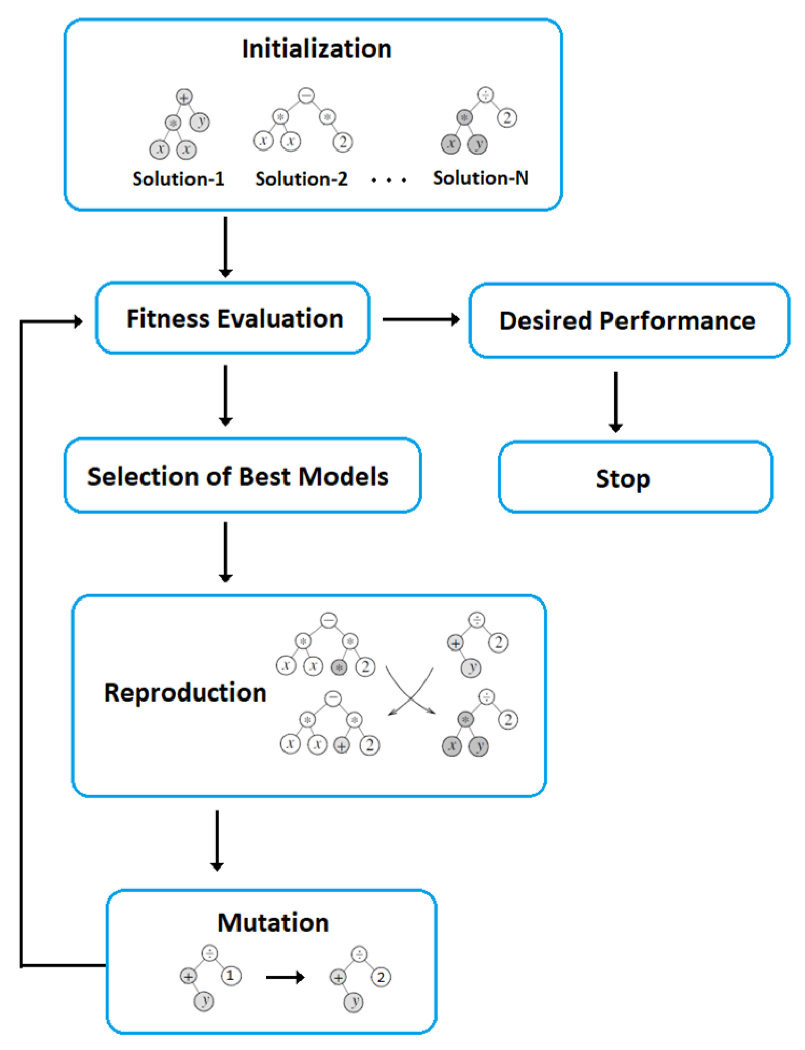
The ML-based symbolic regression method called GEP was employed in this study to generate temperature-based ET equations. GEP was used as the literature suggests that it is highly effective for generating empirical equations [49,50]. The concept of GEP originated from evolutionary algorithms [51], a variant of genetic programming [52]. GEP comprises two main components: the chromosomes and the expression trees expressing the genetic variations encoded in chromosomes. Various genetic operators introduce genetic variations, including mutation, transposition, and recombination. The set of rules in GEP are very simple. The chromosomes of the initial population (program) are randomly generated and presented using expression trees. In this study, ET equations are presented using expression trees. Evolutionary operators are applied to the equations to evolve new expression trees from the initial trees and, thus, new ET equations. The fitness of each equation is evaluated using a statistical metric. The equations found to have better fitness or higher capacities for estimating the observed ET are kept for the next iteration, while others are discarded. The process is repeated until the expected ET equation is obtained with less error than in the ET estimation. A typical process of GEP model development is shown in Figure 3.
The procedure used to develop the GEP model using GEP is as follows:
  • Selection of fitness function or a set of fitness functions. The Nash–Sutcliff Efficiency (NSE) was considered for the fitness function.
  • Selection of a set of terminals and a set of functions. The inputs were selected according to their influence on ET.
  • Creation of chromosomes from the selected terminals and functions.
  • Setting the chromosomal architecture.
  • Selection of the linking function.
  • Selection of genetic operators.
The above-mentioned steps were repeated until the fittest program was achieved. In this research, the GeneXproTools software package was used to perform symbolic regression operations based on Gene Expression Programming (GEP) for modelling ET.

4.2. Temperature-Based ET Methods

This study employed six temperature-based empirical models to assess the skill of the newly developed ET model using GEP. The models were selected based on their applicability worldwide. Table 2 provides the details of the ET models. Further details of the models and their performance in Peninsular Malaysia can be found in Muhammad et al. [16].

4.3. Temperature Downscaling and Projections

In the present study, the model output statistics (MOS) approach [47] was used for the downscaling of GCMs at each station location for the projections of ET. For this purpose, the GCM simulations (historical and future) from four grid points surrounding a meteorological station were interpolated to the station location using the bilinear interpolation method [48]. Interpolated GCM temperatures were compared with in situ temperatures for 1975–2005. The quantile mapping technique was employed to correct bias in GCM simulations using in situ temperatures as the reference. Finally, the bias correcting factors were employed to correct bias in the projected temperatures for 2010–2099.

5. Results & Discussion

5.1. Development of Temperature-Based ET Equations Using GEP

GEP models were calibrated with approximately seventy percent of the data and validated with thirty percent of the data. The GEP algorithm was run for at least 10,000 iterations for the purposes of calibrating and cross-validating the models. The GEP hyperparameters were optimized during cross-validation. Finally, the optimized parameters were used for ET prediction. The GEP models were developed separately for all the ten selection locations of peninsular Malaysia. The obtained models for the Alor Setar station are given in Table 3.

5.2. Performance Evaluation of GEP ET Equations

The accuracy of GEP ET formulas in estimating in situ ET was evaluated at all locations. Four statistical metrics, Nash–Sutcliffe Efficiency (NSE), mean absolute error (MAE), root-mean-square error (RMSE), and modified coefficient agreement (md), were used for this purpose. The results in Table 4 showed the high performance of the GEP estimated ET model at different stations. The NSE value was more than 0.76 at all locations. The MAE and RMSE values were less than 10.1 and 12.1, and md values were more than 0.7 at all stations. This indicates the efficiency of the newly developed ET models for peninsular Malaysia.
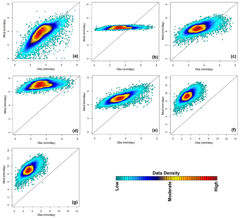
The relative performance of the GEP ET model with the existing temperature-based models was also evaluated. The scatter plot of the in situ and GEP simulated ET is presented in Figure 4. Observed and model-simulated ET data for all locations were merged to generate the scatter plots. The points along the diagonal line indicate the improved performance of the model. The results showed that GEP ET estimated points are more aligned with the diagonal line than the other model. This indicates the improved accuracy of the newly developed equations over the existing ET methods. Therefore, the newly developed models can be used for reliable projections of ET around peninsular Malaysia using the GCM projected temperature.
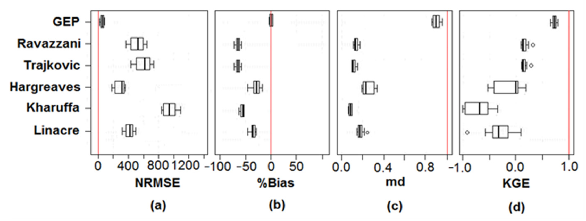
The performance of the models was evaluated using different statistical metrics. The obtained results from different locations are presented using box plots in Figure 5. The results are presented to show the accuracy of the GEP model compared to the existing empirical model and, thus, the capability of the GEP model to reduce uncertainty in estimating ET in Peninsular Malaysia. The vertical red line in the plot indicates the optimum value of the corresponding metric. Therefore, a box close to the ideal line indicates better performance. The results showed the GEP box is much closer to the optimum line than the other models. It indicates the higher performance of GEP compared to the other models.

5.3. Projection of ET

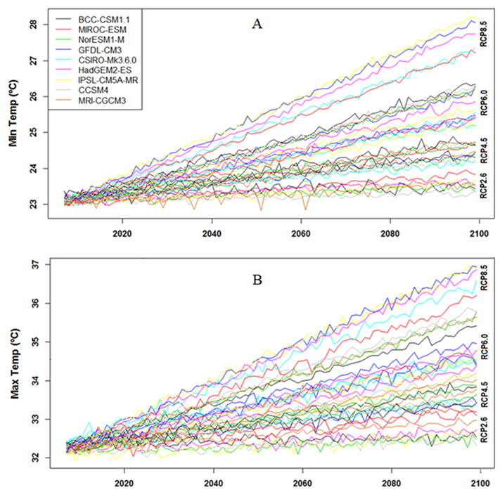
The temperatures projected by all GCMs were integrated to generate ensemble projection. In this study, the multimodel ensemble (MME) projections were obtained by averaging the projections of all GCMs. The MME mean temperature at each station was used to estimate the projected mean change in temperature. The changes in Tmin and Tmax at the Alor Setar station are given in Figure 6 as an example.
The MME mean of the GCM projected temperatures showed a rise in maximum temperature at all locations for all the RCPs. The increasing pattern was similar to that obtained for two other periods, 2010–2039 and 2040–2069. The RCP2.6 projected an increase by 0.00 to 0.41 °C, RCP4.5 by 0.84 to 1.27 °C, RCP6.0 by 1.28 to 1.71 °C, and RCP8.5 by 2.79 to 3.24 °C. A larger rise in minimum temperature was projected in the north and south of the peninsula and at least in the central region of the peninsula. The RCP2.6 projected a rise in minimum temperature by 0.15 to 0.43 °C, RCP4.5 by 0.54 to 1.38 °C, RCP6.0 by 0.92 to 1.77 °C, and RCP8.5 by 2.47 to 3.30 °C.
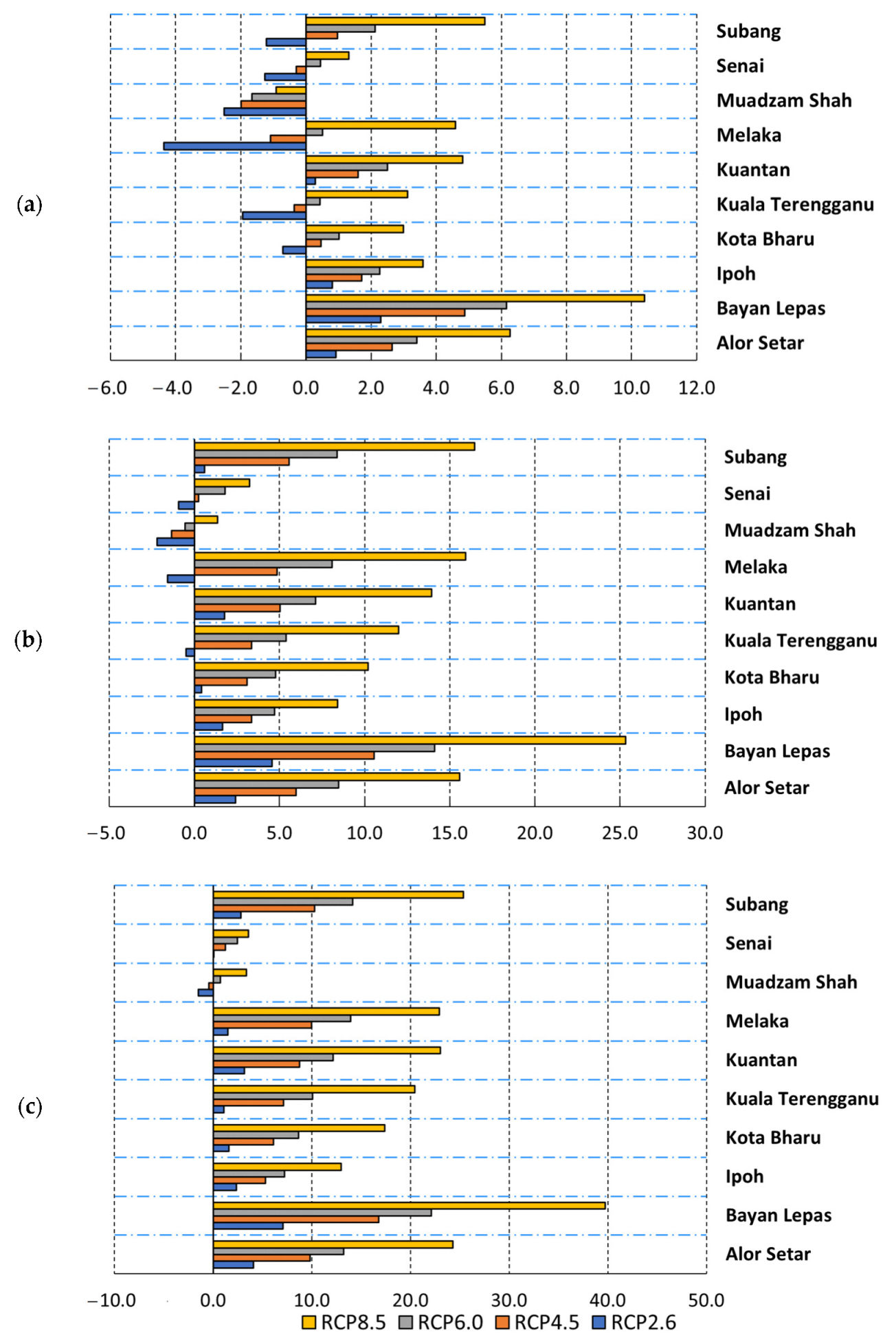
The changes in ET, compared to the historical period (1975–2005), at all studied locations are given in Figure 7. The results show an increase in ET for all RCPs and future time horizons for the stations located northwest of the peninsula. The highest increase was projected for Byan Lepas, located in the northwest, by 2.3–7.06% for RCP2.6, 4.88–16.76% for RCP4.5, 6.16–22.14% for RCP6.0 and 10.39–39.74% for RCP8.5. Stations in other parts of the peninsula showed a decrease in ET for RCP2.6 during 2010–2039. The decrease was found to be higher at the stations located in the central part. For RCP4.5, ET was projected to decrease for all the future periods only at Muadzam Shah station. It decreased at other stations in the central region during 2010–2039 but increased for later periods. The increase was found to be rapid for many stations. For example, it was projected to increase only 0.96% during 2010–2039, but 10.3% during 2070–2099 for RCP4.5. The ET was projected to increase at all stations for all the periods for RCP6.0, except Muadzam Shah. The ET was also projected to increase at all stations for all future periods for RCP8.5, except at Muadzam Shah during 2010–2039. The increase in ET at different stations during 2040–2069 was in the range of 1.35–25.33%, while increases were in the range of 3.35–39.74% during 2070–2099.
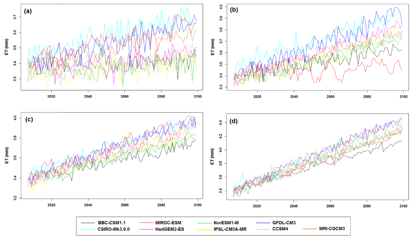
The changes in ET for different RCPs for the whole future period (2010–2099) were plotted to assess the uncertainty in projections. The projected ET at Alor Setar station for different RCPs is shown as an example in Figure 8. Projections by different GCMs represent the uncertainty in projection. For the RCP2.6 and RCP4.5 scenarios, CSIRO-Mk3.6.0 projected a higher increase in ET, while IPSL-CM5A-MR and MIROC-ESM projected the least increase in ET. For RCP6.0 and RCP8.5, GFDL-CM3 projected a higher increase in ET, while BCC-CSM1.1 projected a relatively low increase in ET. The uncertainty in the projected ET was higher for the last part of the projection than in the earlier part. The increase in uncertainty was found to be gradual with time. For example, the uncertainty range in ET projection for RCP6.0 was 3.41–3.58 mm during 2010–2039, 3.56–3.72 mm during 2040–2069, and 3.7–3.88 mm during 2070–2099. The uncertainty in ET projection was also higher for higher RCPs. Therefore, uncertainty in ET projection was found to be highest for RCP8.5 and lowest for RCP2.6. The uncertainty in ET projection for RCP2.6 during 2070–2099 was 3.36–3.67 mm, while it was 3.46–3.89 mm for RCP4.5, 3.70–3.88 mm for RCP6.0, and 4.01–4.31 mm for RCP8.5.

6. Discussion

The present study developed empirical models using GEP for reliable ET estimation and projection using only temperature data. The comparison of the newly developed models showed higher performance in terms of multiple statistical indices compared to the existing widely used temperature-based models. The performance of the GEP models according to some indices showed considerable improvement. For example, the NRMSE (%) of the GEP models was in the range of 7.8 to 19.9 at different locations compared to 198.1–354.1 for the Hargreaves model, which showed the best performance among the five empirical models considered. This indicates a nearly twenty-fold improvement in performance in NRMSE. Similar improvement was noticed in other indices. This indicates the capability of GEP models in estimating ET in Peninsular Malaysia with higher accuracy and less uncertainty.
RCPs are considered to be radiative forcing based on factors contributing to greenhouse gas concentrations, including land use and land cover changes, population growth, and economic evolution [59]. For example, RCP2.6 shows an increase in agricultural land with no change in grassland over time. RCP4.5 shows decreased cropland while increasing in vegetated land at the end of the century [60]. Therefore, the results presented in the study for different RCPs should be interpreted based on global changes in land use that are considered when designing RCPs [61].
This study developed and employed only the temperature-based model considering the ready availability of temperature data. This is also due to their applicability in projecting ET. All GCMs project temperature data for all RCPs. However, this is not the case for other climate variables, like wind speed and solar radiation. Only a few GCMs project those variables but not for all RCPs. Therefore, the equations developed in this study can be used in ET projections for all GCMs and RCPs. This helped us to understand the complete range of uncertainty in ET projections.
The projection of ET using GEP models revealed an overall increase in ET in Peninsular Malaysia for all RCPs. The increases would be higher during 2070–2099 compared to the other periods. The increase would also be higher for higher RCPs than the lower RCPs. Therefore, the largest increase will be for RCP8.5 during 2070–2099, with an areal average of nearly 21%. In contrast, it may slightly decrease in the early period for RCP2.6. However, the average areal decrease is projected at only 1.2%, which is negligible. Uncertainty in the projected ET shows an increase over time. The greater uncertainty was noticed for higher RCPs. Therefore, it can be anticipated that the large projected increase in ET during 2070–2099 for RCP8.5 is more uncertain than the projected decrease in ET for RCP2.6 during 2010–2039.

7. Conclusions

The present study used the symbolic regression method to develop new temperature-based ET models with regard to Peninsular Malaysia for ET estimation and projections for different RCPs. The results indicate that the GEP model developed with only temperature data can estimate ET reliably, which establishes the efficacy of GEP models in estimating daily ET in peninsular Malaysia. The study reports a rise in ET with an increase in temperature in the study area. ET would increase all over the peninsula for all RCPs and future periods, except in the central peninsula for the early (2010–2039) period for mild RCPs. Climate change may affect irrigation, agriculture, and ecology across the globe. The GEP-based method proposed in this study has the potential to be employed for generating reliable ET empirical formulations, which can be used for reliable projections of ET for assessing climate change impacts on different water sectors. The ET projections in Peninsular Malaysia shown in this study could help support adaptation responses for reducing climate change risk. The findings will be useful to different organizations working on natural resource management. The results could also enhance knowledge of climate change and its impact on ET. In the future, GCMs of recently released CMIP6 can be employed in improving the predictions of new scenarios.

Author Contributions

Conceptualization, M.K.I.M., S.S., M.M.H., S.H., T.I., and X.W.; methodology, M.K.I.M. and S.S.; programming, S.S. and M.M.H.; validation, S.H., T.I., and X.W.; formal analysis, M.K.I.M., S.H., and T.I.; resources, M.K.I.M.; data curation, S.S. and T.I.; writing—original draft preparation, M.K.I.M. and S.S.; writing—review and editing, S.H., T.I., and X.W.; visualization, M.K.I.M. and M.M.H.; supervision, S.S. and X.W. All authors have read and agreed to the published version of the manuscript.

Funding

We are grateful to The Belt and Road Special Foundation of the State Key Laboratory of Hydrology-Water Resources and Hydraulic Engineering (2019491311) for providing financial support for this research.

Institutional Review Board Statement

Not applicable.

Informed Consent Statement

Not applicable.

Data Availability Statement

GCM data used in this study are freely available on the websites mentioned in the manuscript.

Acknowledgments

We are grateful to the Program for Climate Model Diagnosis & Intercomparison (PCMDI) of Lawrence Livermore National Laboratory, CA, USA, for publicly providing the GCM simulation data through their web portal.

Conflicts of Interest

The authors declare no conflict of interest.

References

  1. Hamed, M.M.; Khan, N.; Shahid, S.; Muhammad, M.K.I. Ranking of Empirical Evapotranspiration Models in Different Climate Zones of Pakistan. Res. Sq. 2022. [Google Scholar] [CrossRef]
  2. Salehie, O.; Hamed, M.M.; Ismail, T.B.; Shahid, S. Projection of droughts in Amu river basin for shared socioeconomic pathways CMIP6. Theor. Appl. Climatol. 2022, 149, 1009–1027. [Google Scholar] [CrossRef]
  3. Kumar, R.; Jat, M.K.; Shankar, V. Methods to estimate irrigated reference crop evapotranspiration–a review. Water Sci. Technol. 2012, 66, 525–535. [Google Scholar] [CrossRef]
  4. Wigmosta, M.S.; Vail, L.W.; Lettenmaier, D.P. A distributed hydrology-vegetation model for complex terrain. Water Resour. Res. 1994, 30, 1665–1679. [Google Scholar] [CrossRef]
  5. Jhajharia, D.; Kumar, R.; Dabral, P.P.; Singh, V.P.; Choudhary, R.R.; Dinpashoh, Y. Reference evapotranspiration under changing climate over the Thar Desert in India. Meteorol. Appl. 2015, 22, 425–435. [Google Scholar] [CrossRef]
  6. Ashfaq, M.; Bowling, L.C.; Cherkauer, K. Influence of climate model biases and daily-scale temperature and precipitation events on hydrological impacts assessment: A case study of the United States. J. Geophys. Res. 2010, 115, D14116. [Google Scholar] [CrossRef]
  7. Kumar, R.; Kumar, M. Evaluation of reference evapotranspiration models using single crop coefficient method and lysimeter data. Indian J. Agric. Sci. 2017, 87, 350–354. [Google Scholar]
  8. Shiru, M.S.; Chung, E.-S.; Shahid, S. Empirical Model for the Assessment of Climate Change Impacts on Spatial Pattern of Water Availability in Nigeria BT-Intelligent Data Analytics for Decision-Support Systems in Hazard Mitigation: Theory and Practice of Hazard Mitigation; Deo, R.C., Samui, P., Kisi, O., Yaseen, Z.M., Eds.; Springer: Singapore, 2021; pp. 405–427. ISBN 978-981-15-5772-9. [Google Scholar]
  9. Adnan, R.M.; Heddam, S.; Yaseen, Z.M.; Shahid, S.; Kisi, O.; Li, B. Prediction of Potential Evapotranspiration Using Temperature-Based Heuristic Approaches. Sustainability 2021, 13, 297. [Google Scholar] [CrossRef]
  10. Jerin, J.N.; Islam, H.M.T.; Islam, A.R.M.T.; Shahid, S.; Hu, Z.; Badhan, M.A.; Chu, R.; Elbeltagi, A. Spatiotemporal trends in reference evapotranspiration and its driving factors in Bangladesh. Theor. Appl. Climatol. 2021, 144, 793–808. [Google Scholar] [CrossRef]
  11. Vishwakarma, D.K.; Pandey, K.; Kaur, A.; Kushwaha, N.L.; Kumar, R.; Ali, R.; Elbeltagi, A.; Kuriqi, A. Methods to estimate evapotranspiration in humid and subtropical climate conditions. Agric. Water Manag. 2022, 261, 107378. [Google Scholar] [CrossRef]
  12. Hamed, M.M.; Salem, M.; Shamsuddin, N.; Tarmizi, S. Thermal bioclimatic indicators over Southeast Asia: Present status and future projection using CMIP6. Environ. Sci. Pollut. Res. 2022, 1–20. [Google Scholar] [CrossRef] [PubMed]
  13. Alamgir, M.; Shahid, S.; Hazarika, M.K.; Nashrrullah, S.; Harun, S.B.; Shamsudin, S. Analysis of Meteorological Drought Pattern During Different Climatic and Cropping Seasons in Bangladesh. JAWRA J. Am. Water Resour. Assoc. 2015, 51, 794–806. [Google Scholar] [CrossRef]
  14. Salehie, O.; Ismail, T.B.; Hamed, M.M.; Shahid, S.; Idlan Muhammad, M.K. Projection of Hot and Cold Extremes in the Amu River Basin of Central Asia using GCMs CMIP6. Stoch. Environ. Res. Risk Assess. 2022, 1–22. [Google Scholar] [CrossRef]
  15. Bashir, T.; Kumar, R. Simulation of Modeling of Water Ecohydrologic Dynamics in a Multilayer Root Zone under Protected Conditions in the Temperate Region of India. J. Hydrol. Eng. 2017, 22, 5017020. [Google Scholar] [CrossRef]
  16. Muhammad, M.K.I.; Nashwan, M.S.; Shahid, S.; Ismail, T.B.; Song, Y.H.; Chung, E.S. Evaluation of empirical reference evapotranspiration models using compromise programming: A case study of Peninsular Malaysia. Sustainability 2019, 11, 4267. [Google Scholar] [CrossRef]
  17. Tukimat, N.N.A.N.A.; Harun, S.; Shahid, S. Comparison of different methods in estimating potential évapotranspiration at Muda Irrigation Scheme of Malaysia. J. Agric. Rural Dev. Trop. Subtrop. 2012, 113, 77–85. [Google Scholar]
  18. Pour, S.H.; Wahab, A.K.A.; Shahid, S.; Ismail, Z. Bin Changes in reference evapotranspiration and its driving factors in peninsular Malaysia. Atmos. Res. 2020, 246, 105096. [Google Scholar] [CrossRef]
  19. Muhammad, M.K.I.; Shahid, S.; Ismail, T.; Harun, S.; Kisi, O.; Yaseen, Z.M. The development of evolutionary computing model for simulating reference evapotranspiration over Peninsular Malaysia. Theor. Appl. Climatol. 2021, 144, 1419–1434. [Google Scholar] [CrossRef]
  20. Courault, D.; Seguin, B.; Olioso, A. Review on estimation of evapotranspiration from remote sensing data: From empirical to numerical modeling approaches. Irrig. Drain. Syst. 2005, 19, 223–249. [Google Scholar] [CrossRef]
  21. Liou, Y.A.; Kar, S.K. Evapotranspiration estimation with remote sensing and various surface energy balance algorithms-a review. Energies 2014, 7, 2821–2849. [Google Scholar] [CrossRef]
  22. Zhang, K.; Kimball, J.S.; Running, S.W. A review of remote sensing based actual evapotranspiration estimation. WIREs Water 2016, 3, 834–853. [Google Scholar] [CrossRef]
  23. Zhan, X.; Fang, L.; Yin, J.; Schull, M.; Liu, J.; Hain, C.; Anderson, M.; Kustas, W.; Kalluri, S. Remote Sensing of Evapotranspiration for Global Drought Monitoring. Glob. Drought Flood 2021, 29–46. [Google Scholar] [CrossRef]
  24. Ahmadi, F.; Nazeri Tahroudi, M.; Mirabbasi, R.; Kumar, R. Spatiotemporal analysis of precipitation and temperature concentration using PCI and TCI: A case study of Khuzestan Province, Iran. Theor. Appl. Climatol. 2022, 149, 743–760. [Google Scholar] [CrossRef]
  25. Sobh, M.T.; Nashwan, M.S.; Amer, N. High Resolution Reference Evapotranspiration for Arid Egypt: Comparative analysis and evaluation of empirical and artificial intelligence models. Res. Sq. 2022. [Google Scholar] [CrossRef]
  26. Ye, L.; Zahra, M.M.A.; Al-Bedyry, N.K.; Yaseen, Z.M. Daily scale evapotranspiration prediction over the coastal region of southwest Bangladesh: New development of artificial intelligence model. Stoch. Environ. Res. Risk Assess. 2021, 36, 451–471. [Google Scholar] [CrossRef]
  27. Nandagiri, L.; Kovoor, G.M. Performance Evaluation of Reference Evapotranspiration Equations across a Range of Indian Climates. J. Irrig. Drain. Eng. 2006, 132, 238–249. [Google Scholar] [CrossRef]
  28. Wei, G.; Zhang, X.; Ye, M.; Yue, N.; Kan, F. Bayesian performance evaluation of evapotranspiration models based on eddy covariance systems in an arid region. Hydrol. Earth Syst. Sci. 2019, 23, 2877–2895. [Google Scholar] [CrossRef]
  29. Penman, H.L. Natural evaporation from open water, bare soil and grass. In Proceedings of the Royal Society of London; The Royal Society London: London, UK, 1948; Volume 193, pp. 120–145. [Google Scholar]
  30. Salman, S.A.; Hamed, M.M.; Shahid, S.; Ahmed, K.; Sharafati, A.; Asaduzzaman, M.; Ziarh, G.F.; Ismail, T.; Chung, E.-S.; Wang, X.-J.; et al. Projecting spatiotemporal changes of precipitation and temperature in Iraq for different shared socioeconomic pathways with selected Coupled Model Intercomparison Project Phase 6. Int. J. Climatol. 2022, 1–19. [Google Scholar] [CrossRef]
  31. Hamed, M.M.; Nashwan, M.S.; Shahid, S.; Ismail, T.B.; Wang, X.J.; Dewan, A.; Asaduzzaman, M. Inconsistency in historical simulations and future projections of temperature and rainfall: A comparison of CMIP5 and CMIP6 models over Southeast Asia. Atmos. Res. 2022, 265, 105927. [Google Scholar] [CrossRef]
  32. Hamed, M.M.; Nashwan, M.S.; Shahid, S. A novel selection method of CMIP6 GCMs for robust climate projection. Int. J. Climatol. 2022, 42, 4258–4272. [Google Scholar] [CrossRef]
  33. Hamed, M.M.; Nashwan, M.S.; Shahid, S. Inter-comparison of Historical Simulation and Future Projection of Rainfall and Temperature by CMIP5 and CMIP6 GCMs Over Egypt. Int. J. Climatol. 2022, 42, 4316–4332. [Google Scholar] [CrossRef]
  34. Salehie, O.; Hamed, M.M.; Ismail, T.; Tam, T.H.; Shahid, S. Selection of CMIP6 GCM with Projection of Climate Over The Amu Darya River Basin. Res. Sq. 2021, 1–27. [Google Scholar] [CrossRef]
  35. Pour, S.H.; Wahab, A.K.A.; Shahid, S. Physical-empirical models for prediction of seasonal rainfall extremes of Peninsular Malaysia. Atmos. Res. 2020, 233, 104720. [Google Scholar] [CrossRef]
  36. Jing, W.; Yaseen, Z.M.; Shahid, S.; Saggi, M.K.; Tao, H.; Kisi, O.; Salih, S.Q.; Al-Ansari, N.; Chau, K.-W. Implementation of evolutionary computing models for reference evapotranspiration modeling: Short review, assessment and possible future research directions. Eng. Appl. Comput. fluid Mech. 2019, 13, 811–823. [Google Scholar] [CrossRef]
  37. Pan, S.; Pan, N.; Tian, H.; Friedlingstein, P.; Sitch, S.; Shi, H.; Arora, V.K.; Haverd, V.; Jain, A.K.; Kato, E.; et al. Evaluation of global terrestrial evapotranspiration using state-of-the-art approaches in remote sensing, machine learning and land surface modeling. Hydrol. Earth Syst. Sci. 2020, 24, 1485–1509. [Google Scholar] [CrossRef]
  38. Carter, C.; Liang, S. Evaluation of ten machine learning methods for estimating terrestrial evapotranspiration from remote sensing. Int. J. Appl. Earth Obs. Geoinf. 2019, 78, 86–92. [Google Scholar] [CrossRef]
  39. Dou, X.; Yang, Y. Evapotranspiration estimation using four different machine learning approaches in different terrestrial ecosystems. Comput. Electron. Agric. 2018, 148, 95–106. [Google Scholar] [CrossRef]
  40. Granata, F. Evapotranspiration evaluation models based on machine learning algorithms—A comparative study. Agric. Water Manag. 2019, 217, 303–315. [Google Scholar] [CrossRef]
  41. Kiafar, H.; Babazadeh, H.; Marti, P.; Kisi, O.; Landeras, G.; Karimi, S.; Shiri, J. Evaluating the generalizability of GEP models for estimating reference evapotranspiration in distant humid and arid locations. Theor. Appl. Climatol. 2017, 130, 377–389. [Google Scholar] [CrossRef]
  42. Mehdizadeh, S.; Behmanesh, J.; Khalili, K. Using MARS, SVM, GEP and empirical equations for estimation of monthly mean reference evapotranspiration. Comput. Electron. Agric. 2017, 139, 103–114. [Google Scholar] [CrossRef]
  43. Estrada-Flores, S.; Merts, I.; De Ketelaere, B.; Lammertyn, J. Development and validation of “grey-box” models for refrigeration applications: A review of key concepts. Int. J. Refrig. 2006, 29, 931–946. [Google Scholar] [CrossRef]
  44. Kazemi, M.H.; Majnooni-Heris, A.; Kisi, O.; Shiri, J. Generalized gene expression programming models for estimating reference evapotranspiration through cross-station assessment and exogenous data supply. Environ. Sci. Pollut. Res. 2021, 28, 6520–6532. [Google Scholar] [CrossRef] [PubMed]
  45. Barzkar, A.; Shahabi, S.; Niazmradi, S.; Madadi, M.R. A comparative study of remote sensing and gene expression programming for estimation of evapotranspiration in four distinctive climates. Stoch. Environ. Res. Risk Assess. 2021, 35, 1437–1452. [Google Scholar] [CrossRef]
  46. Tangang, F.T. Low frequency and quasi-biennial oscillations in the Malaysian precipitation anomaly. Int. J. Climatol. 2001, 21, 1199–1210. [Google Scholar] [CrossRef]
  47. Pour, S.H.; Shahid, S.; Chung, E.S.; Wang, X.J. Model output statistics downscaling using support vector machine for the projection of spatial and temporal changes in rainfall of Bangladesh. Atmos. Res. 2018, 213, 149–162. [Google Scholar] [CrossRef]
  48. Hamed, M.M.; Nashwan, M.S.; Shahid, S. Performance Evaluation of Reanalysis Precipitation Products in Egypt using Fuzzy Entropy Time Series Similarity Analysis. Int. J. Climatol. 2021, 41, 5431–5446. [Google Scholar] [CrossRef]
  49. Nait Amar, M. Prediction of hydrate formation temperature using gene expression programming. J. Nat. Gas. Sci. Eng. 2021, 89, 103879. [Google Scholar] [CrossRef]
  50. Chu, H.-H.; Khan, M.A.; Javed, M.; Zafar, A.; Ijaz Khan, M.; Alabduljabbar, H.; Qayyum, S. Sustainable use of fly-ash: Use of gene-expression programming (GEP) and multi-expression programming (MEP) for forecasting the compressive strength geopolymer concrete. Ain Shams Eng. J. 2021, 12, 3603–3617. [Google Scholar] [CrossRef]
  51. Kotanchek, M.E.; Vladislavleva, E.Y.; Smits, G.F. Symbolic Regression Via Genetic Programming as a Discovery Engine: Insights on Outliers and Prototypes BT-Genetic Programming Theory and Practice VII; Riolo, R., O’Reilly, U.-M., McConaghy, T., Eds.; Springer: Boston, MA, USA, 2010; pp. 55–72. ISBN 978-1-4419-1626-6. [Google Scholar]
  52. Koza, J.R. Evolution of subsumption using genetic programming. In Proceedings of the First European Conference on Artificial Life; MIT Press: Cambridge, MA, USA, 1992; pp. 110–119. [Google Scholar]
  53. Doorenbos, J.; Pruitt, W.O. Crop water requirements. FAO Irrigation and Drainage Paper 24. In Land and Water Development Division; FAO: Rome, Italy, 1977; Volume 144. [Google Scholar]
  54. Linacre, E.T. A simple formula for estimating evaporation rates in various climates, using temperature data alone. Agric. Meteorol. 1977, 18, 409–424. [Google Scholar] [CrossRef]
  55. Kharrufa, N.S. Simplified equation for evapotranspiration in arid regions. Beiträge Hydrol. 1985, 5, 39–47. [Google Scholar]
  56. Hargreaves, G.; Samani, Z. Reference Crop Evapotranspiration from Temperature. Appl. Eng. Agric. 1985, 1, 96–99. [Google Scholar] [CrossRef]
  57. Trajkovic, S. Hargreaves versus Penman-Monteith under Humid Conditions. J. Irrig. Drain. Eng. 2007, 133, 38–42. [Google Scholar] [CrossRef]
  58. Ravazzani, G.; Corbari, C.; Morella, S.; Gianoli, P.; Mancini, M. Modified Hargreaves-Samani Equation for the Assessment of Reference Evapotranspiration in Alpine River Basins. J. Irrig. Drain. Eng. 2012, 138, 592–599. [Google Scholar] [CrossRef]
  59. Taylor, K.E.; Stouffer, R.J.; Meehl, G.A. An overview of CMIP5 and the experiment design. Bull. Am. Meteorol. Soc. 2012, 93, 485–498. [Google Scholar] [CrossRef]
  60. Van Vuuren, D.P.; Edmonds, J.; Kainuma, M.; Riahi, K.; Thomson, A.; Hibbard, K.; Hurtt, G.C.; Kram, T.; Krey, V.; Lamarque, J.F.; et al. The representative concentration pathways: An overview. Clim. Chang. 2011, 109, 5–31. [Google Scholar] [CrossRef]
  61. IPCC. Climate Change 2013: The Physical Science Basis; IPCC: Cambridge, UK; New York, NY, USA, 2013. [Google Scholar]
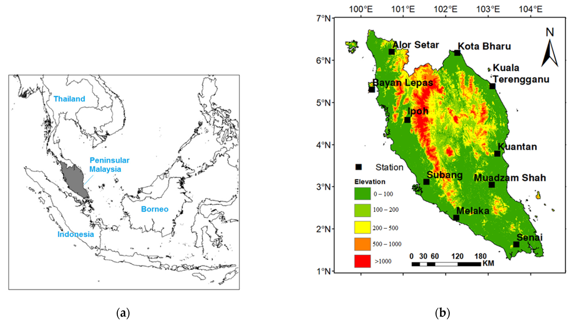
Figure 1. (a) Location of peninsular Malaysia on the map of Southeast Asia; (b) Geographical position of peninsular Malaysia. The topography and location of the meteorological stations are also provided.
Water 14 02858 g001
Figure 2. Variability in monthly average (a) daily maximum, mean, and minimum temperatures; (b) evapotranspiration in the study area from 1975 to 2014.
Water 14 02858 g002
Figure 3. The procedure used to generate ET empirical equations using gene expression programming (GEP).
Water 14 02858 g003
Figure 4. Density scatter plots showing the relative performance of the GEP (a) ET model compared to (b) FAO Blaney-Criddle, (c) Linacre, (d) Kharrufa, (e) Hargreaves and Samani, (f) Trajkovic, and (g) Ravazzani ET models.
Water 14 02858 g004
Figure 5. Box plot of (a) normalized root mean square error (%), (b) percentage bias, (c) modified index of agreement, and (d) Kling-Gupta efficiency in estimating ET by different empirical models. The vertical red line in the plot indicates the ideal line.
Water 14 02858 g005
Figure 6. Projection of annual daily average of (A) minimum and (B) maximum temperature in Alor Setar stations for RCP2.6, RCP4.5, RCP6.0 and RCP8.5.
Water 14 02858 g006
Figure 7. Projected changes (%) in the annual average of daily ET for three future periods: (a) 2010–2039; (b) 2040–2069; and (c) 2070–2099 compared to the historical period (1975–2005) for four RCPs at different locations of peninsular Malaysia.
Water 14 02858 g007
Figure 8. Projections of the annual average of daily ET at Alor Setar station for (a) RCP2.6; (b) RCP4.5; (c) RCP6.0; and (d) RCP8.5 for the period 2010–2099.
Water 14 02858 g008
Table 1. List of CMIP5 GCMs employed in this research.
Model Developing InstituteModel NameResolution
(Lon × Lat)
Beijing Climate Center, ChinaBCC-CSM1.12.8° × 2.8°
National Center for Atmospheric Research, USACCSM41.25° × 0.94°
Met Office Hadley Centre, UKHadGEM2-ES1.87° × 1.25°
Atmosphere and Ocean Research Institute, The University of Tokyo, JapanMIROC-ESM2.8° × 2.8°
Bjerknes Centre for Climate Research, Norwegian Meteorological Institute, NorwayNorESM1-M2.5° × 1.9°
Geophysical Fluid Dynamics Laboratory, USAGFDL-CM32.5° × 2.0°
Commonwealth Scientific and Industrial Research Organization, AustraliaCSIRO-Mk3.6.01.86° × 1.87°
Institut Pierre Simon Laplace, FranceIPSL-CM5A-MR1.26° × 2.5°
Meteorological Research Institute, JapanMRI-CGCM31.12° × 1.12°
Table 2. The temperature-based empirical ET formulations considered in this study.
NoModelInput ParameterEquation
1FAO Blaney-Criddle [53]Tmean p ( 0.46 T mean + 8.13 )
2Linacre [54]Tmean 700 ( T mean ± 0.006 z ) 100 L + 15 ( T mean T d ) 80 T mean
3Kharrufa [55]Tmean 0.34 pT mean 1.30
4Hargreaves and Samani [56]Tmean, Tmin, Tmax, Ra ( 0.0023 R a 2.45 ) TD 0.5 ( T mean + 17.8 )
5Trajkovic [57]Tmean, Tmin, Tmax, Ra ( 0.0023 R a ) TD 0.424 ( T mean + 17.8 )
6Ravazzani [58]Tmean, Tmin, Tmax, Ra ( 0.817 + 0.00022 z ) ( 0.0023 R a ) ( TD 0.5 ) ( T mean + 17.8 )
TD is daily temperature range (°C); Tmean is the average temperature (°C); Ra is the extraterrestrial radiation (MJ/m2/day).
Table 3. The GEP models developed at all the stations in Peninsular Malaysia.
Station NameModel
Alor Setar [(0.708527 + Tmax + (Tmax/−0.570404)) × ((Tmax + Tmin) × (0.708527/Tmax))] + [0.271 × Tmin−4.310577] + [Tmax−((39.983448 + Tmin)/(6.337066 + Tmin))]
Bayan Lepas [−2.659455/(Tmin + ((Tmin + Tmax) × (−2.659455/Tmax)))] − [9.144561] + [((Tmax + 2.659455) × Tmax)/(Tmin + 1.002563 + 2 × Tmax)]
Ipoh [−9.89798−Tmin] + [(2 × Tmax−Tmin + 2.245544)/8.36405] + [Tmin + 7.706391]
Kota Bharu((Tmax/4.688568) − (4.688568/Tmin) − 4.688568) + (−1.946625/((Tmin×
−1.946625) + Tmax + 5.589417)) + (Tmax/(Tmin − ((Tmin + Tmax)/(Tmin^2))))
Kuala Terenggannu(Tmax/5.405304) + ((2 × Tmax + 2 × Tmin)/((Tmax^0.13211) + (Tmax × 5.950409)))+
((Tmin + Tmax)/(12.843872 − Tmax))
Kuantan(((Tmin × −1.63205) + (Tmin/−1.63205))/((Tmin × Tmax)/(Tmin − 1.63205))) +
(((−4.044677/(Tmin/Tmax)) + 1.682221 − Tmax)/−4.044677) − 4.384247
Melaka((−8.459076 + Tmax)/Tmax) + ((Tmax − Tmin)/((2 × Tmax)/(0.269501 + Tmax))) +
(−8.391388/(Tmin − 18.419738))
Muadzam Shah [((Tmin − Tmax)/(7.168945 − Tmax))/((7.168945/Tmax) − 7.411835)] + [((−6.097015/Tmin) − (4.724793 + Tmin))/((Tmax × 4.724793) + (−6.097015/Tmax))] + [((Tmin − Tmax)/(−9.070129 − Tmax))/(1.893555/Tmin)]
Senai [(−5.88443 − Tmin + Tmax)/(−3.50461 + 2Tmin)] + [−10.39233/(Tmin − 14.90024)] + [2Tmax2/Tmin2]
Subang [−4.079162/Tmin] + [(6.476776 − Tmin)/(Tmax/(Tmin − Tmax))] +
[−14.214936/(−12.751648 + Tmin)]
Table 4. Performance of temperature-based ET model developed using GEP.
Station NameNSEMAERMSEmd
Alor Setar0.984.77.91.0
Senai0.945.47.60.9
Bayan Lepas0.926.68.90.9
Ipoh0.817.39.30.7
Muadzam Shah0.796.98.90.8
Subang0.766.17.60.7
Kuantan0.993.34.81.0
Melaka0.946.19.30.9
Kota Bharu0.8710.112.10.8
Kuala Terenggannu0.955.810.30.9
Publisher’s Note: MDPI stays neutral with regard to jurisdictional claims in published maps and institutional affiliations.