Author Contributions
Conceptualization, E.S. and J.-H.C.; methodology, E.S. and N.V.A.P.; software, N.V.A.P. and E.S.; validation, E.S. and N.V.A.P.; formal analysis, E.S.; investigation, E.S., J.-H.C. and N.V.A.P.; resources, J.-H.C.; data curation E.S. and N.V.A.P.; writing—original draft preparation, E.S.; writing—review and editing, J.-H.C. and N.V.A.P.; visualization, N.V.A.P.; supervision, J.-H.C.; project administration, J.-H.C.; funding acquisition, J.-H.C. All authors have read and agreed to the published version of the manuscript.
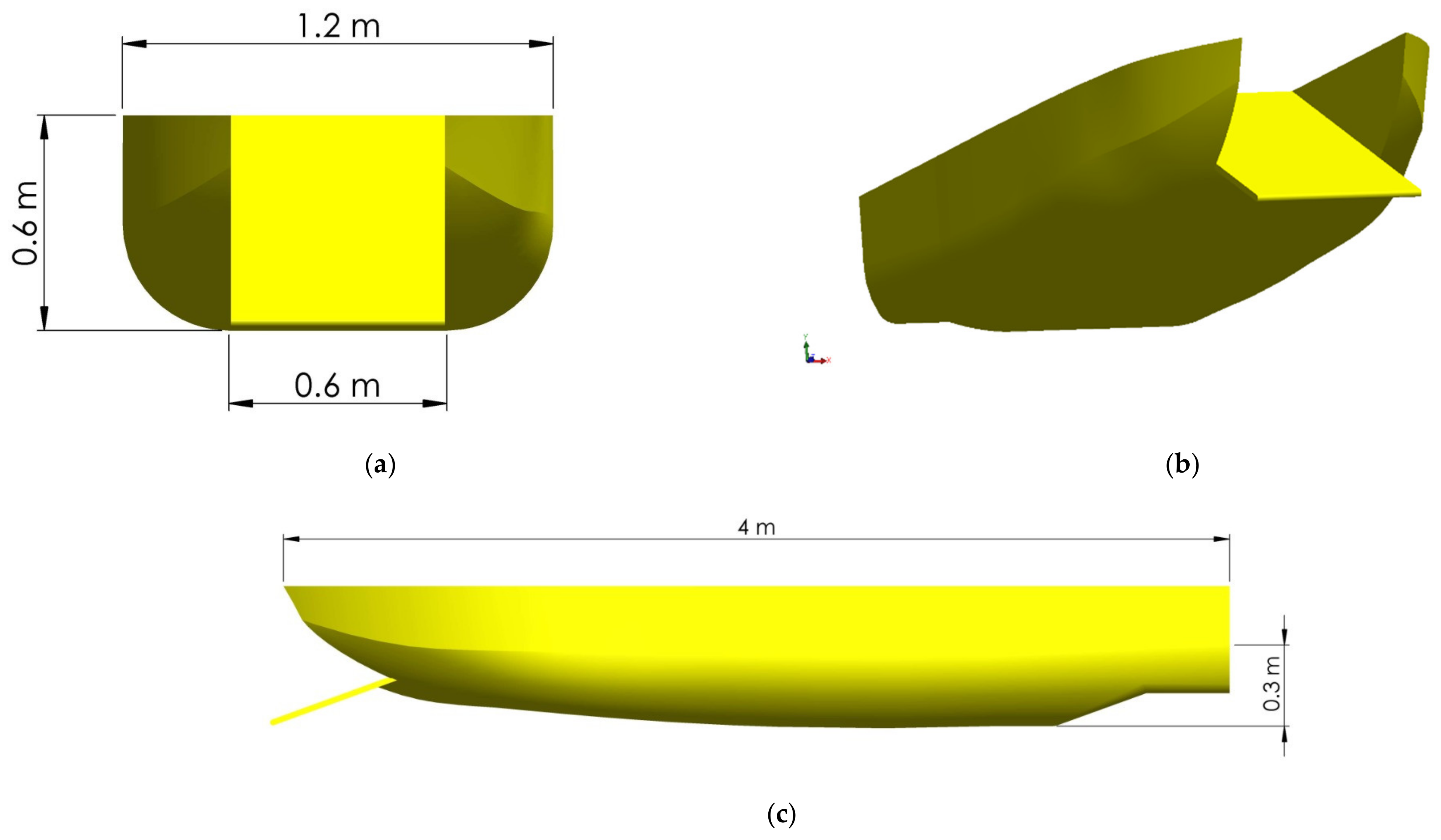
Figure 1.
Monohull model: (a) front view of round bilge, (b) 3D view of round bilge, and (c) side view.
Figure 1.
Monohull model: (a) front view of round bilge, (b) 3D view of round bilge, and (c) side view.
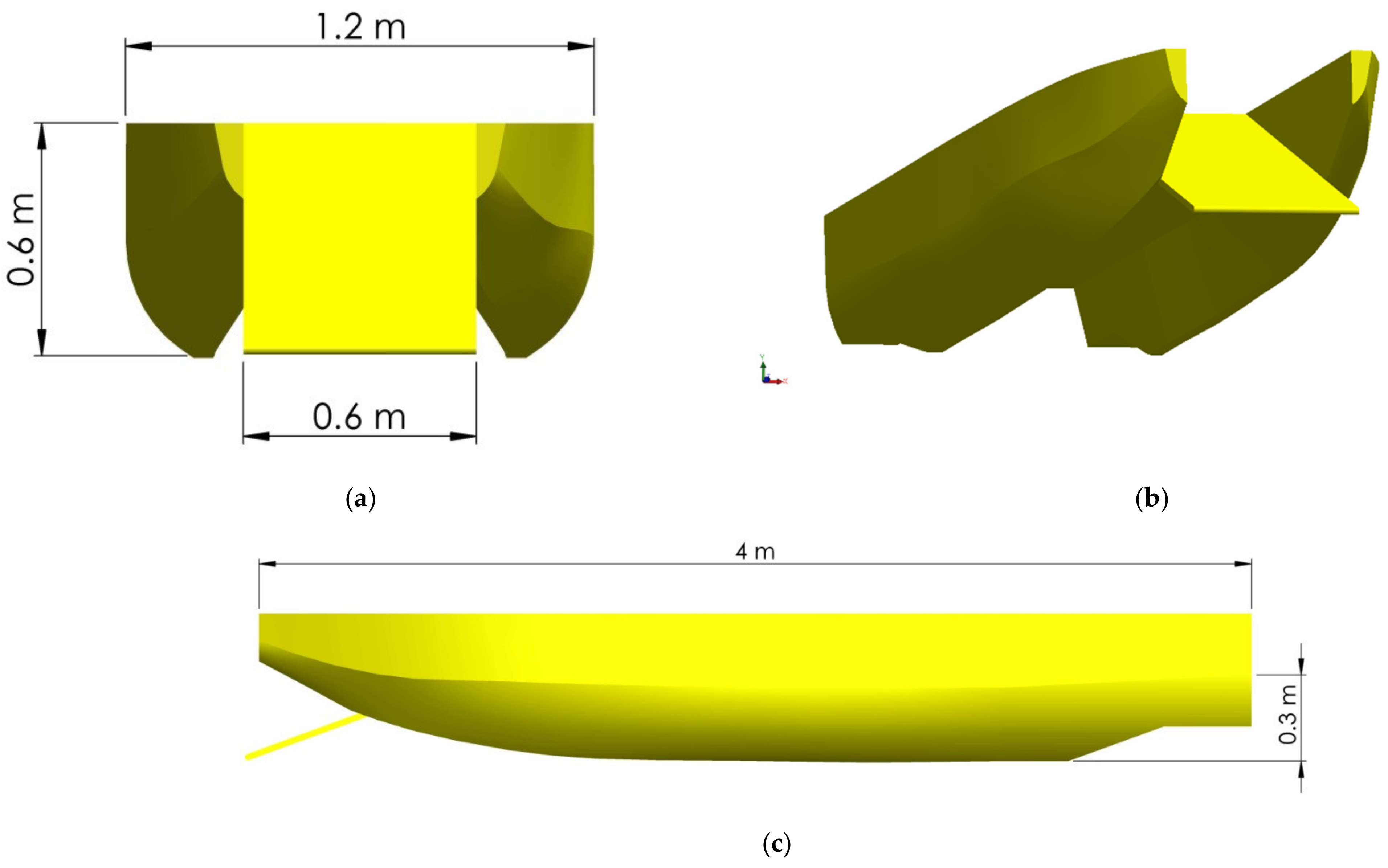
Figure 2.
Catamaran model: (a) front view of inner flat hull, (b) 3D view of inner flat hull, (c) side view.
Figure 2.
Catamaran model: (a) front view of inner flat hull, (b) 3D view of inner flat hull, (c) side view.
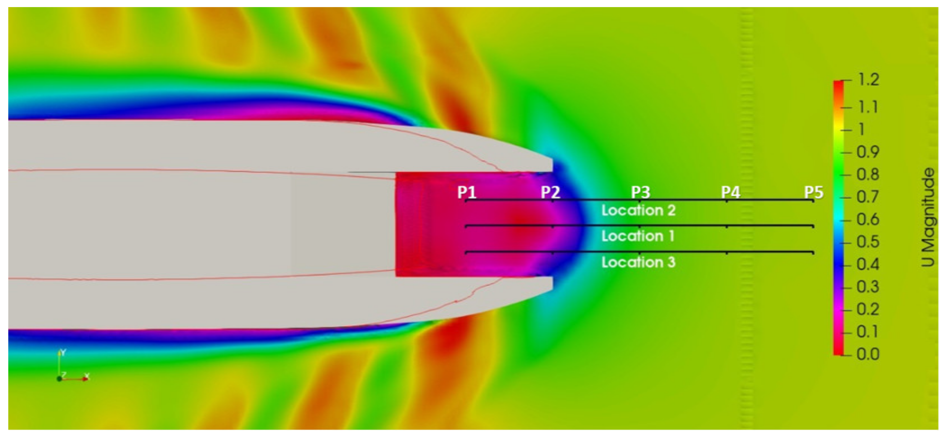
Figure 3.
Location of probes.
Figure 3.
Location of probes.
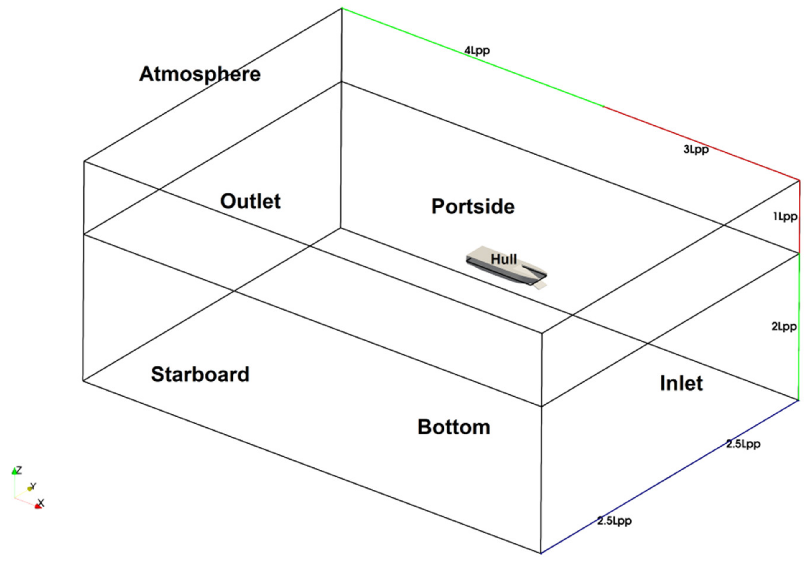
Figure 4.
Fluid domain and boundaries used to model.
Figure 4.
Fluid domain and boundaries used to model.
Figure 5.
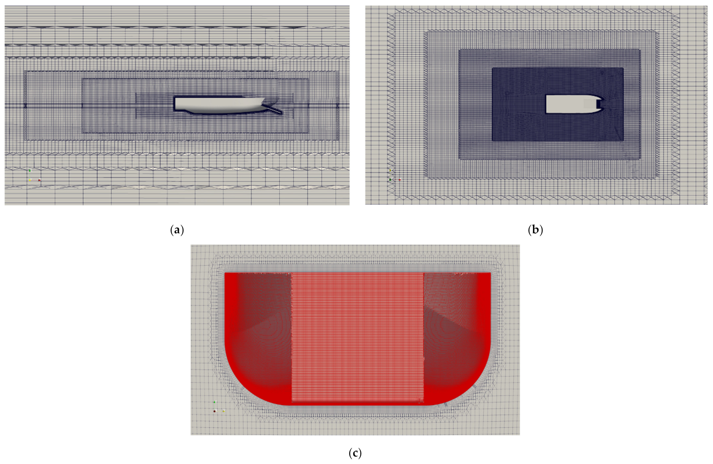
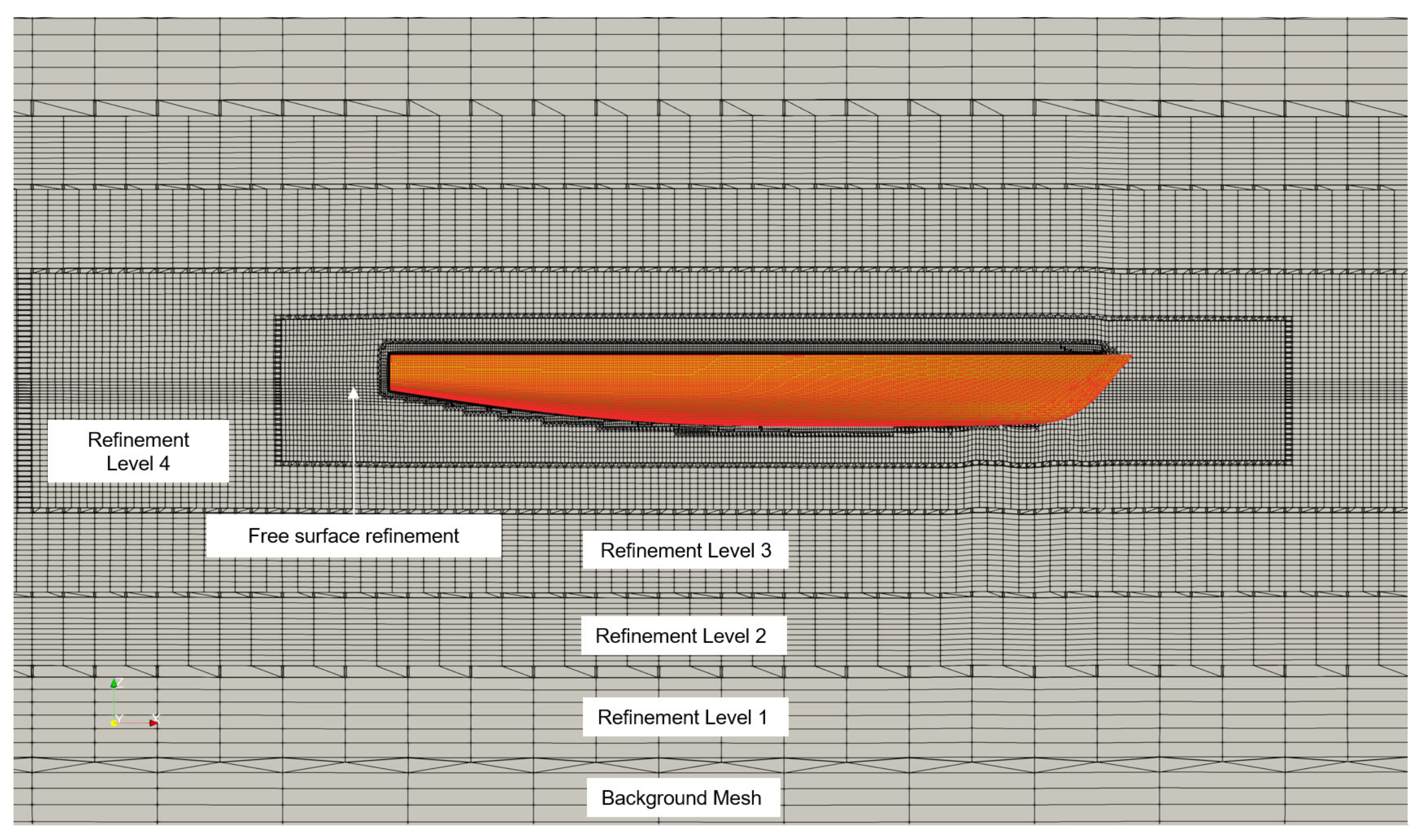
Meshing in fluid domain with refinement levels: (a) side view model, (b) top view, (c) front view.
Figure 5.
Meshing in fluid domain with refinement levels: (a) side view model, (b) top view, (c) front view.
Figure 6.
The actual number of surface prism layers generated around the ship model using the snappyHexMesh tool: (a) surface layers, (b) yPlus.
Figure 6.
The actual number of surface prism layers generated around the ship model using the snappyHexMesh tool: (a) surface layers, (b) yPlus.
Figure 7.
Meshing result on the Delft catamaran 372 model.
Figure 7.
Meshing result on the Delft catamaran 372 model.
Figure 8.
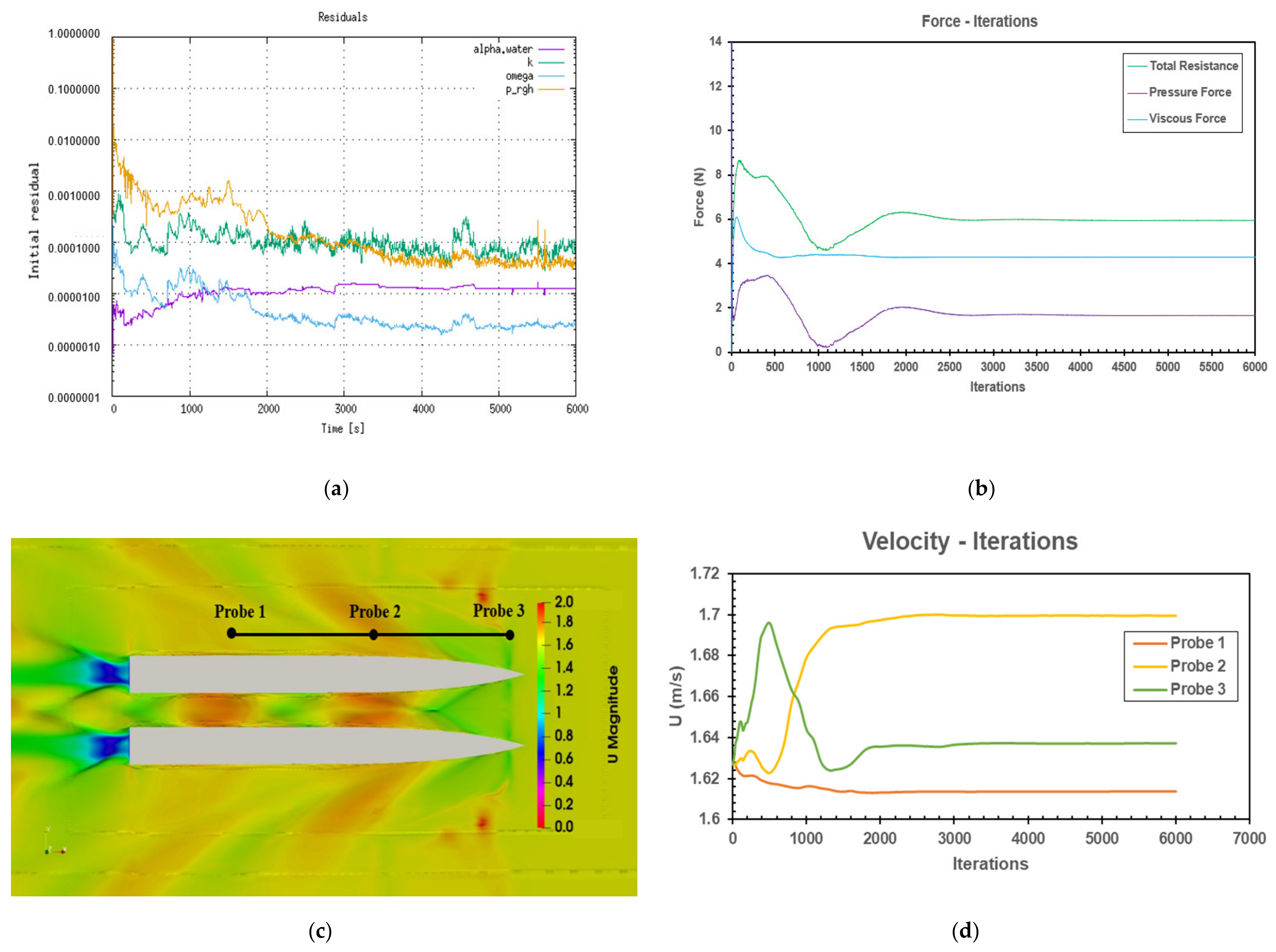
Residual and force components evolution: (a) residual iteration evolution, (b) force components iteration evolution using 2,196,512 cells, (c) location of velocity sampling, (d) velocity convergence.
Figure 8.
Residual and force components evolution: (a) residual iteration evolution, (b) force components iteration evolution using 2,196,512 cells, (c) location of velocity sampling, (d) velocity convergence.
Figure 9.
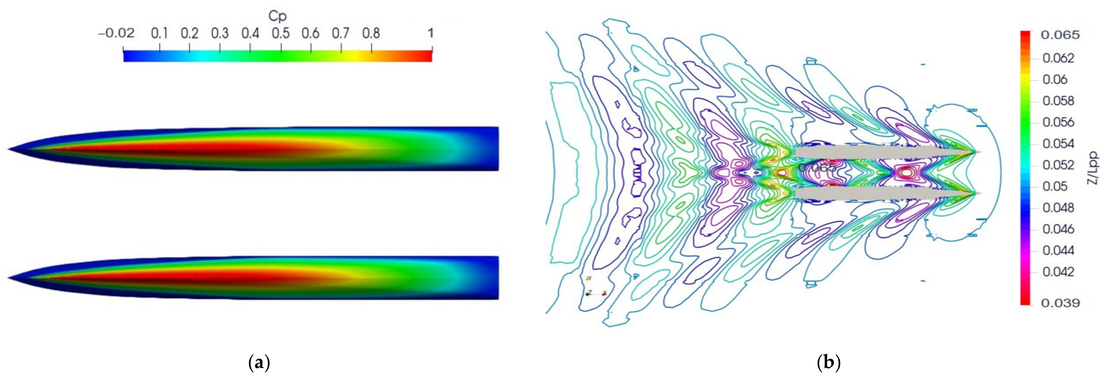
Pressure coefficient distribution (a) and wave patterns (b) on Delft catamaran 372 surface at Froude number 0.3.
Figure 9.
Pressure coefficient distribution (a) and wave patterns (b) on Delft catamaran 372 surface at Froude number 0.3.
Figure 10.
Distribution of wave generated around round-bilge monohull 1 m/s: (a) wave elevation, (b) wave profile along body.
Figure 10.
Distribution of wave generated around round-bilge monohull 1 m/s: (a) wave elevation, (b) wave profile along body.
Figure 11.
Distribution of wave generated around inner flat catamaran at 1 m/s speed: (a) wave elevation, (b) wave profile along body.
Figure 11.
Distribution of wave generated around inner flat catamaran at 1 m/s speed: (a) wave elevation, (b) wave profile along body.
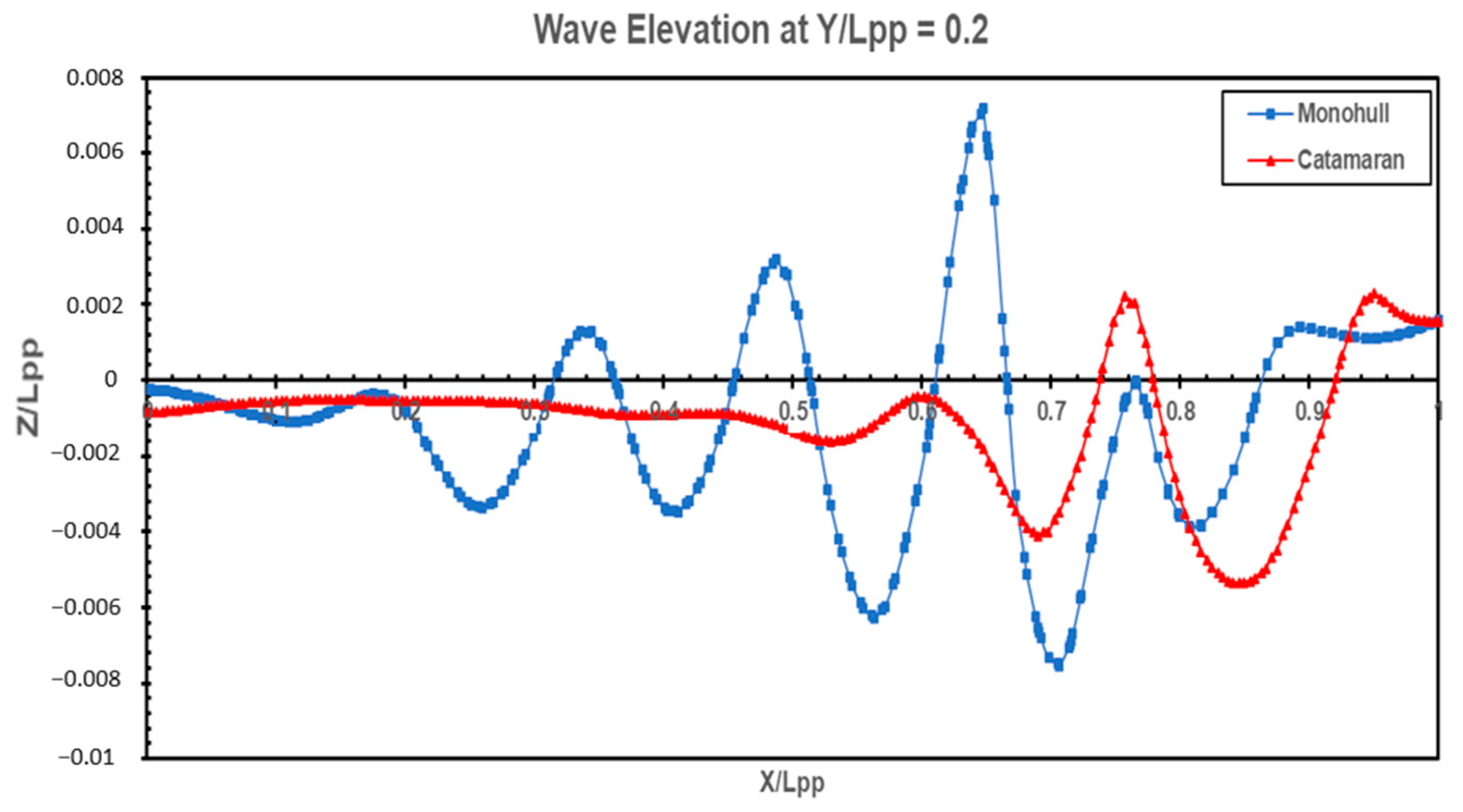
Figure 12.
Wave elevation at Y/Lpp = 0.2 at 1 m/s speed.
Figure 12.
Wave elevation at Y/Lpp = 0.2 at 1 m/s speed.
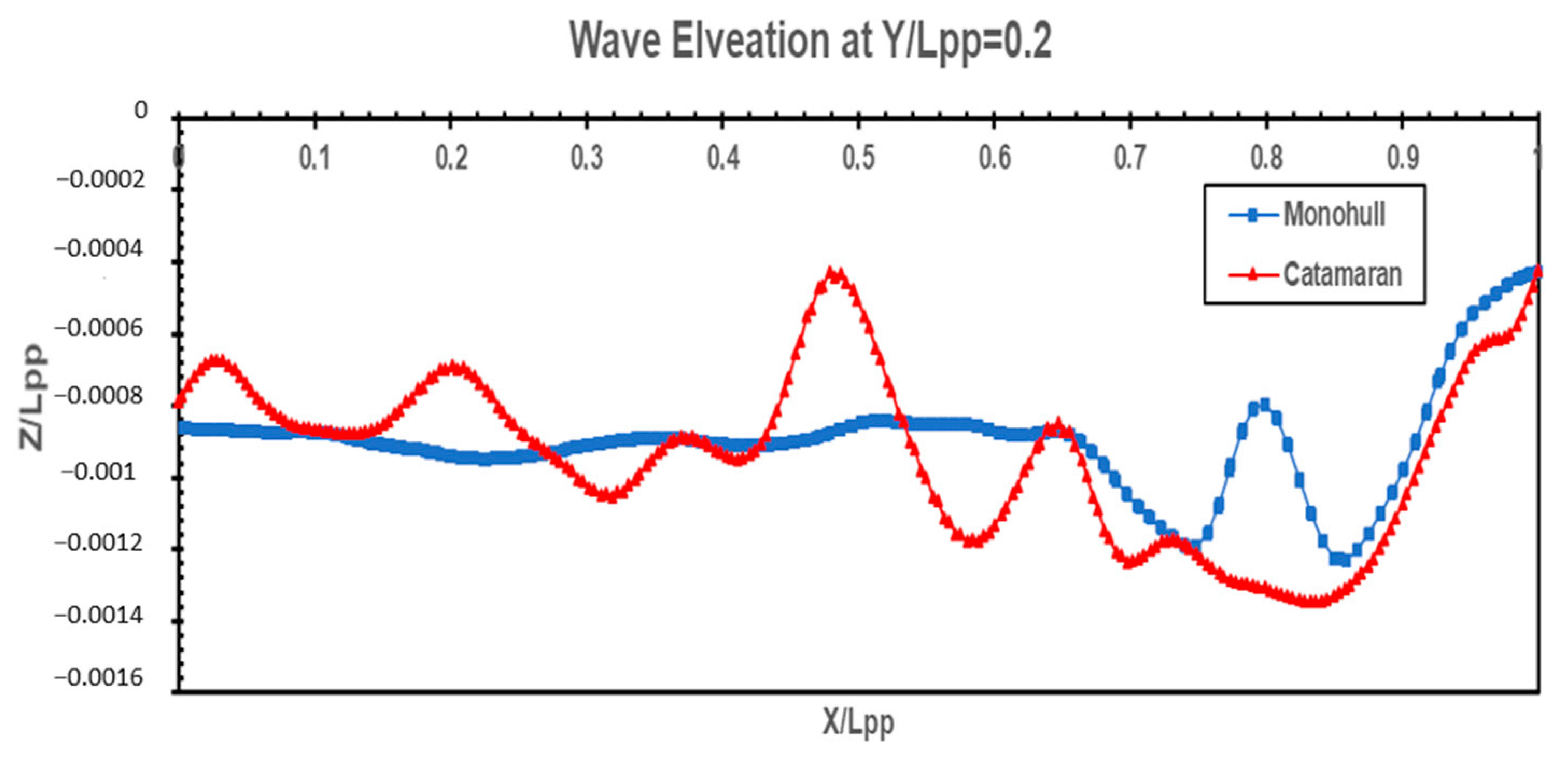
Figure 13.
Wave elevation at Y/Lpp = 0.2 at 0.5 m/s speed.
Figure 13.
Wave elevation at Y/Lpp = 0.2 at 0.5 m/s speed.
Figure 14.
Turbulent kinetic energy at 1 m/s speed: (a) monohull, (b) catamaran.
Figure 14.
Turbulent kinetic energy at 1 m/s speed: (a) monohull, (b) catamaran.
Figure 15.
Turbulent intensity at 1 m/s speed: (a) monohull, (b) catamaran.
Figure 15.
Turbulent intensity at 1 m/s speed: (a) monohull, (b) catamaran.
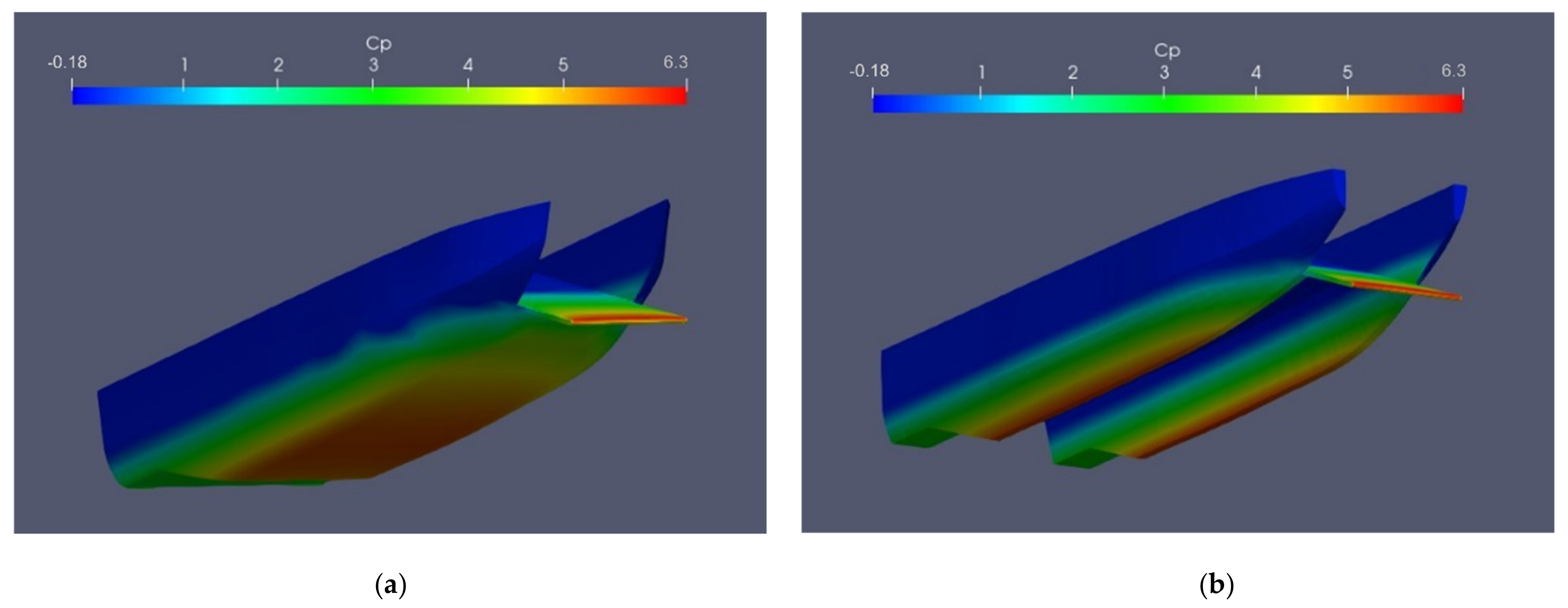
Figure 16.
Pressure coefficient distribution on ship surface at 1 m/s: (a) monohull, (b) catamaran.
Figure 16.
Pressure coefficient distribution on ship surface at 1 m/s: (a) monohull, (b) catamaran.
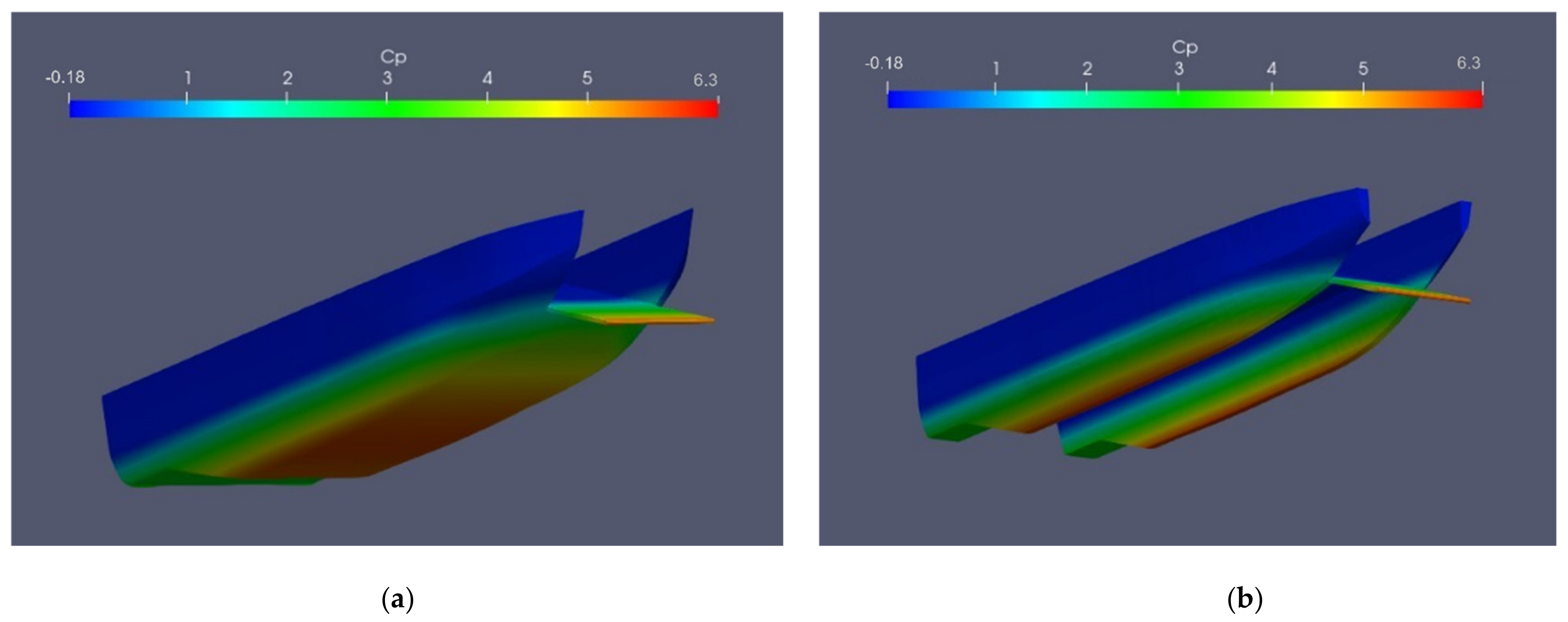
Figure 17.
Pressure coefficient distribution on ship surface at 0.5 m/s: (a) monohull, (b) catamaran.
Figure 17.
Pressure coefficient distribution on ship surface at 0.5 m/s: (a) monohull, (b) catamaran.
Figure 18.
Flow pattern at 1 m/s speed: (a) round-bilge monohull, (b) inner flat catamaran.
Figure 18.
Flow pattern at 1 m/s speed: (a) round-bilge monohull, (b) inner flat catamaran.
Figure 19.
Flow pattern at 0.5 m/s speed: (a) round-bilge monohull, (b) inner flat catamaran.
Figure 19.
Flow pattern at 0.5 m/s speed: (a) round-bilge monohull, (b) inner flat catamaran.
Figure 20.
Velocity contour at 1 m/s speed: (a) round-bilge monohull, (b) inner flat catamaran.
Figure 20.
Velocity contour at 1 m/s speed: (a) round-bilge monohull, (b) inner flat catamaran.
Figure 21.
Velocity contour at 0.5 m/s speed: (a) round-bilge monohull, (b) inner flat catamaran.
Figure 21.
Velocity contour at 0.5 m/s speed: (a) round-bilge monohull, (b) inner flat catamaran.
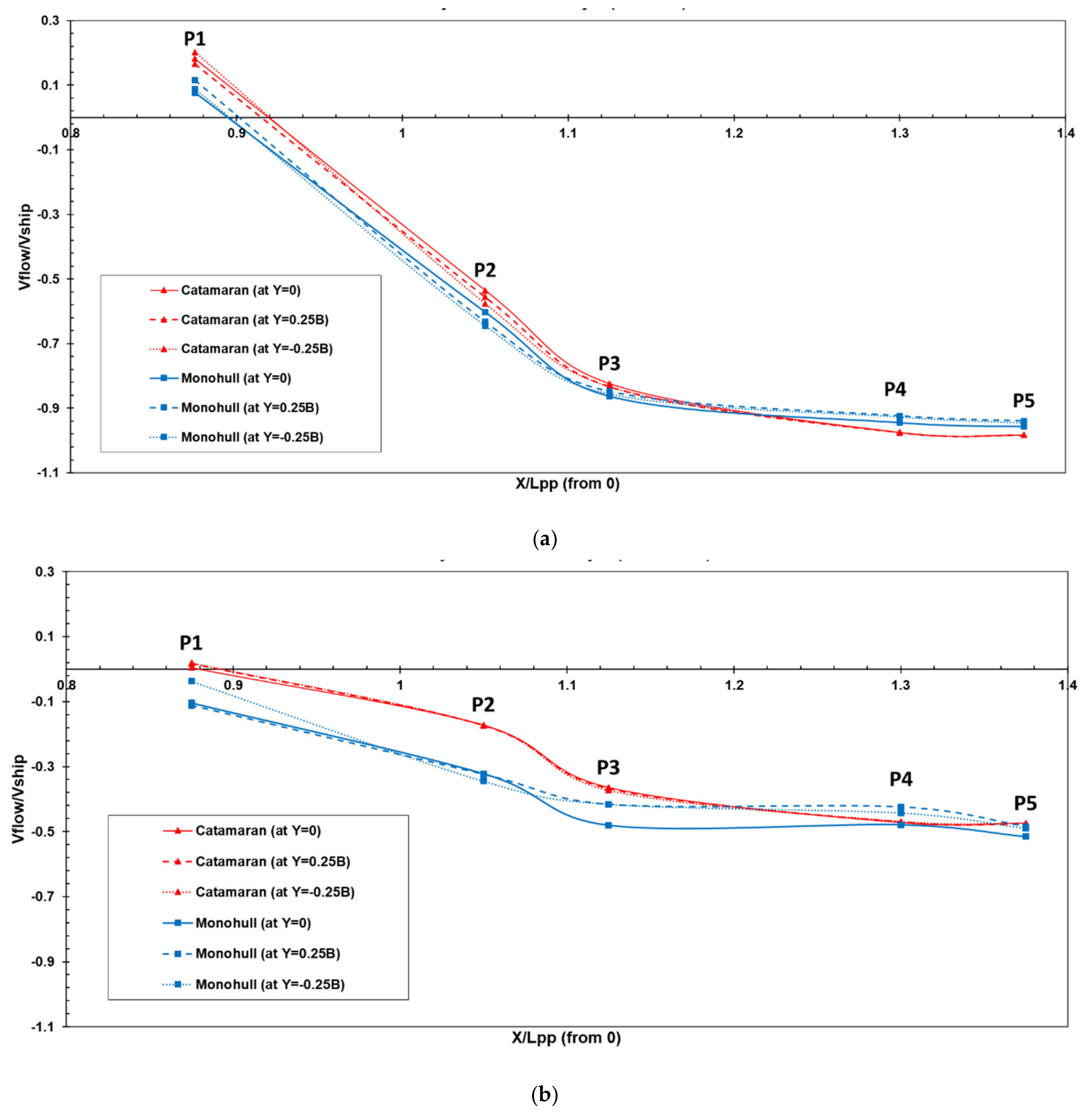
Figure 22.
Velocity flow at probes: (a) 1 m/s speed, (b) 0.5 m/s speed.
Figure 22.
Velocity flow at probes: (a) 1 m/s speed, (b) 0.5 m/s speed.
Table 1.
Ship main dimensions [
10,
23].
Table 1.
Ship main dimensions [
10,
23].
| Parameter | Symbol | Monohull | Catamaran |
|---|
| Length overall [m] | Loa | 4.000 | 4.000 |
| Length perpendicular [m] | Lpp | 3.950 | 3.950 |
| Length of water line [m] | Lwl | 3.858 | 3.858 |
| Maximum breadth [m] | B | 1.200 | 1.200 |
| Height [m] | H | 0.600 | 0.600 |
| Draft [m] | T | 0.300 | 0.300 |
| Wetted surface area [m2] | WSA | 6.232 | 5.723 |
| Conveyor length [m] | Lc | 1.625 | 1.625 |
| Conveyor angle [o] | La | 20 | 20 |
| Conveyor wide [m] | Lw | 0.600 | 0.600 |
| Volume displacement | m3 | 0.90 | 0.36 |
| Block coefficient | - | 0.625 | 0.25 |
Table 2.
Control points’ locations measured from in front of ship conveyors.
Table 2.
Control points’ locations measured from in front of ship conveyors.
| Probes | X (m) | Y1 | Y2 | Y3 | Z |
|---|
| P1 | 3.5 | 0 | 0.15 | −0.15 | 0 |
| P2 | 4.2 | 0 | 0.15 | −0.15 | 0 |
| P3 | 4.5 | 0 | 0.15 | −0.15 | 0 |
| P4 | 5.2 | 0 | 0.15 | −0.15 | 0 |
| P5 | 5.5 | 0 | 0.15 | −0.15 | 0 |
Table 3.
Boundary conditions.
Table 3.
Boundary conditions.
| Parameter | Velocity | Dynamic Pressure | α. Water | Omega | k |
|---|
| Inlet | fixedValue | fixedFluxPressure | fixedValue | fixedValue | fixedValue |
| Starboard | zeroGradient | zeroGradient | variableHeightFlowRate | zeroGradient | zeroGradient |
| Portside | zeroGradient | zeroGradient | zeroGradient | zeroGradient | zeroGradient |
| Atmosphere | pressureInletOutletVelocity | totalPressure | inletOutlet | inletOutlet | inletOutlet |
| Bottom | zeroGradient | zeroGradient | fixedValue | zeroGradient | eroGradient |
| Outlet | outletPhaseMeanVelocity | zeroGradient | variableHeightFlowRate | inletOutlet | inletOutlet |
| Hull | movingWallVelocity | fixedFluxPressure | zeroGradient | omegaWallFunction | qRWallFunction |
Table 4.
Average and standard deviation of force components vs. grid density for Delft catamaran 372 at Fr = 0.3.
Table 4.
Average and standard deviation of force components vs. grid density for Delft catamaran 372 at Fr = 0.3.
| Grid Density | Number of Cells | Pressure | Viscous | Total | Experiment Value | % Error |
|---|
| Coarse | 737,304 | 5.38 | 8.22 | 13.60 | 12.77 | 6.5 |
| Medium | 2,196,512 | 3.46 | 8.56 | 12.02 | 12.77 | 5.8 |
| Fine | 4,400,870 | 2.62 | 11.71 | 14.33 | 12.77 | 12.2 |
Table 5.
Comparison of numerical results and experimental data.
Table 5.
Comparison of numerical results and experimental data.
| | Vs (m/s) | Fn | Re | Rt (N) | Ct × 10−3 |
|---|
| Experiment [30,31] | 1.627 | 0.3 | 4.882 × 10⁶ | 12.77 | 4.961 |
| Prelimina [34] | 1.637 | 0.3 | 4.882 × 10⁶ | 14.00 | 5.523 |
| Present study | 1.627 | 0.3 | 4.882 × 10⁶ | 12.02 | 4.555 |
| Percentage error with experiment (%) | - | - | - | 5.843 | 8.18 |
| Percentage error with Prelimina (%) | - | - | - | 12.85 | 17.52 |
Table 6.
The uncertainty analysis for monohull model.
Table 6.
The uncertainty analysis for monohull model.
| Grid | No. of Cells | | | | | | | |
|---|
| Fine | 7,735,423 | 141.51 | 1.59 | | | | | |
| Medium | 3,143,952 | 143.10 | 6.38 | 0.2492 | 4.009 | 0.35 | 1.41 |
| Coarse | 945,286 | 149.48 | | | | | |
Table 7.
The uncertainty analysis for catamaran model.
Table 7.
The uncertainty analysis for catamaran model.
| Grid | No. of Cells | | | | | | | |
|---|
| Fine | 5,877,600 | 136.95 | −0.07 | | | | | |
| Medium | 3,143,952 | 136.87 | −1.19 | 0.0623 | 8.007 | 0.0042 | 0.0042 |
| Coarse | 1,777,139 | 135.68 | | | | | |
