Assessment of Diffuse Pollution Loads in Peri-Urban Rivers—Analysis of the Accuracy of Estimation Based on Monthly Monitoring Data

Abstract

Diffuse pollution loads are crucial information for water resource management, and yet field data are often scarce, implying questionable accuracy in load estimates made from low-frequency water quality monitoring. This paper aimed to characterize diffuse pollution in a stream of a mixed-land-cover watershed with a significant portion of urbanized areas through intensive monitoring and to perform a comparative analysis between the loads estimated by pollutant rating curves obtained by regression and the estimates using monthly water quality data, which is the method currently used. Continuous rainfall and flow monitoring was conducted between 2019 and 2021, and samples were collected during flood events and the dry period for water quality analysis. Flood events were found to induce an increase in suspended solids (TSS) and COD concentrations, while inorganic nitrogen (Inorg-N) concentrations were higher in the dry season. Flood characteristics showed a positive correlation with solids and COD event mean concentrations (EMCs) and negative with Inorg-N EMCs, while rainfall characteristics, such as antecedent dry days and intensity, correlate positively with all these pollutants. The rating curves performed well for total load estimation in low discharge events (R² and NSE > 0.8), except for total phosphorus (TP) loads. Estimated annual unit loads found for the watershed were 2 ton TSS/ha.year, 300 kg COD/ha.year, 5 kg Inorg-N/ha.year, and 0.5 kg TP/ha.year, showing high pollution generated in the watershed. Finally, a comparison with estimates based on monthly monitoring data indicated that this method is sufficient for accurate nutrient loads, but not for TSS and COD loads, which require continuous monitoring to improve the accuracy of estimation.

1. Introduction

Urban growth causes numerous challenges for the management of water resources, including those related to stormwater management [1]. The impermeabilization of surfaces generates, among other changes in the hydrological cycle, an increase in the volume of runoff from precipitation and the peak flow that reaches the receiving bodies [2]. In addition to the impact on flows, water bodies that receive water discharges from urban areas suffer great deterioration in the quality of their water due to diffuse pollution from surface runoff, which mobilizes pollutants accumulated on surfaces [3,4]. In Brazil, separate sewage and stormwater systems are generally adopted, although irregular discharges into one system or the other are frequent, which increases the problem of diffuse pollution.

Incorporating the effects of diffuse pollution in the planning and management of watersheds is important to mitigate its impacts and preserve the receiving bodies [5]. For this purpose, it is necessary to understand the phenomenon in a wide variety of locations, which implies the need for monitoring. Specific monitoring programs for the study of diffuse pollution are necessary to provide important information on pollutant loads, which can support the implementation of control measures [6]. However, diffuse pollution is episodic in nature, depending on the occurrence of rainfall and surface conditions, and therefore implies monitoring complexity [7]. To determine the pollutant loads, measurements of flow and concentration are required under different conditions, especially in flood events, but water quality sampling is not as simple as flow monitoring and can be both more expensive and time consuming [8].

Research for the characterization of diffuse pollution has been carried out for some years around the world and at a variety of scales, from parcels, with the study of surface runoff before it is collected [9], at points through the constructed drainage networks [10,11], to studies in streams that receive stormwater discharges, within watersheds with different land cover characteristics [12,13,14,15]; however, they are still scarce. At the watershed scale, the contribution of diffuse pollution is mainly assessed by comparing the conditions of the water body in the dry period and the conditions found during flood events. Flood events result in changes (in general, increases) in the concentrations of several pollutants in streams, such as sediments, organic matter, nutrients, and metals [16,17,18,19,20], indicating that high flows are associated with high pollution loads.

Quantifying diffuse pollution in terms of loads is important for evaluating the impact on water quality accumulated over time [7]. For the estimation of pollution loads from areas or periods without observed data, methods from the most simple, such as adopting load export coefficients or typical pollutant concentrations generally based on land use [21,22] or fitting equations by regression [21,23,24], to the more complex ones, which include hydrological and water quality modeling with the application of equations to represent various processes, among them the accumulation and washing of pollutants on the surface [24,25,26], can be used. Process-based models require large amounts of input data and, depending on the objective, the efforts required may not be worth it [24].

Equations that relate pollutant load or concentration to hydrological variables and watershed characteristics, obtained by regression methods, are commonly used for the estimation of pollutant loads in situations of limited availability of water quality data [27]. These equations are also called rating curves and their application in the context of water pollution originates in sediment estimation, with pollutant load generally being related to the rate or volume of water discharge, since the first is a function of the last and they are variables that are generally well correlated [21]. Although rating curves are widely used for sediment estimation [28,29], research has also investigated the application for estimation of other pollutants, such as nutrients [30,31]. The application of these curves may be more suitable for estimating cumulative pollution loads over longer periods, of the order of years, being associated with smaller errors [32,33].

In the Federal District, located in the center of Brazil, Paranoá Lake, which is, in fact, an artificial reservoir, is an important source of water for the region and suffers the impacts of the effluents from the urban settlements around it, receiving both discharges of stormwater and treated domestic sewage. The lake has already presented the occurrence of cyanobacterial blooms due to eutrophication [34] and experiences silting in the branches that receive the adjacent watersheds [35,36,37], experiencing, since its formation in 1960, the loss of hundreds of meters in length and meters in depth in the main branches. One of these watersheds and the one that contributes the most to Paranoá Lake in terms of outflow and water pollution is the Riacho Fundo watershed [35,38,39], which drains the waters of several urbanized areas, some still lacking sanitary sewage system coverage, and which use individual septic tanks. Research developed on surface runoff from areas within the Riacho Fundo waters and in one of its main tributaries identified a strong influence of diffuse pollution on the deterioration of the watershed’s water quality [11,20,40,41].

The modeling of nutrient loads contributing to Paranoá Lake through the Riacho Fundo watershed has already been performed by Nunes [38] with a daily time step and without focusing on diffuse pollution as a specific objective. Moreover, the author reports difficulties related to the lack of suspended solids monitoring data and the low frequency of nitrogen and phosphorus monitoring. In the Federal District, the available water quality data obtained by the institutions responsible for monitoring are of monthly or less periodicity, which is a limitation in the estimation of pollution loads, especially those that incorporate the effect of diffuse pollution.

In this context, this work aimed to analyze the errors incurred in estimating loads of sediments and pollutants transported by the Riacho Fundo stream based on monthly measurement of water quality parameters and daily flows, through comparative analysis with the estimation performed with 10 min flow data and rating curves of water quality parameters obtained through monitoring in flood events and also with sampling campaigns in the dry period, carried out between 2019 and 2021.

2. Materials and Methods

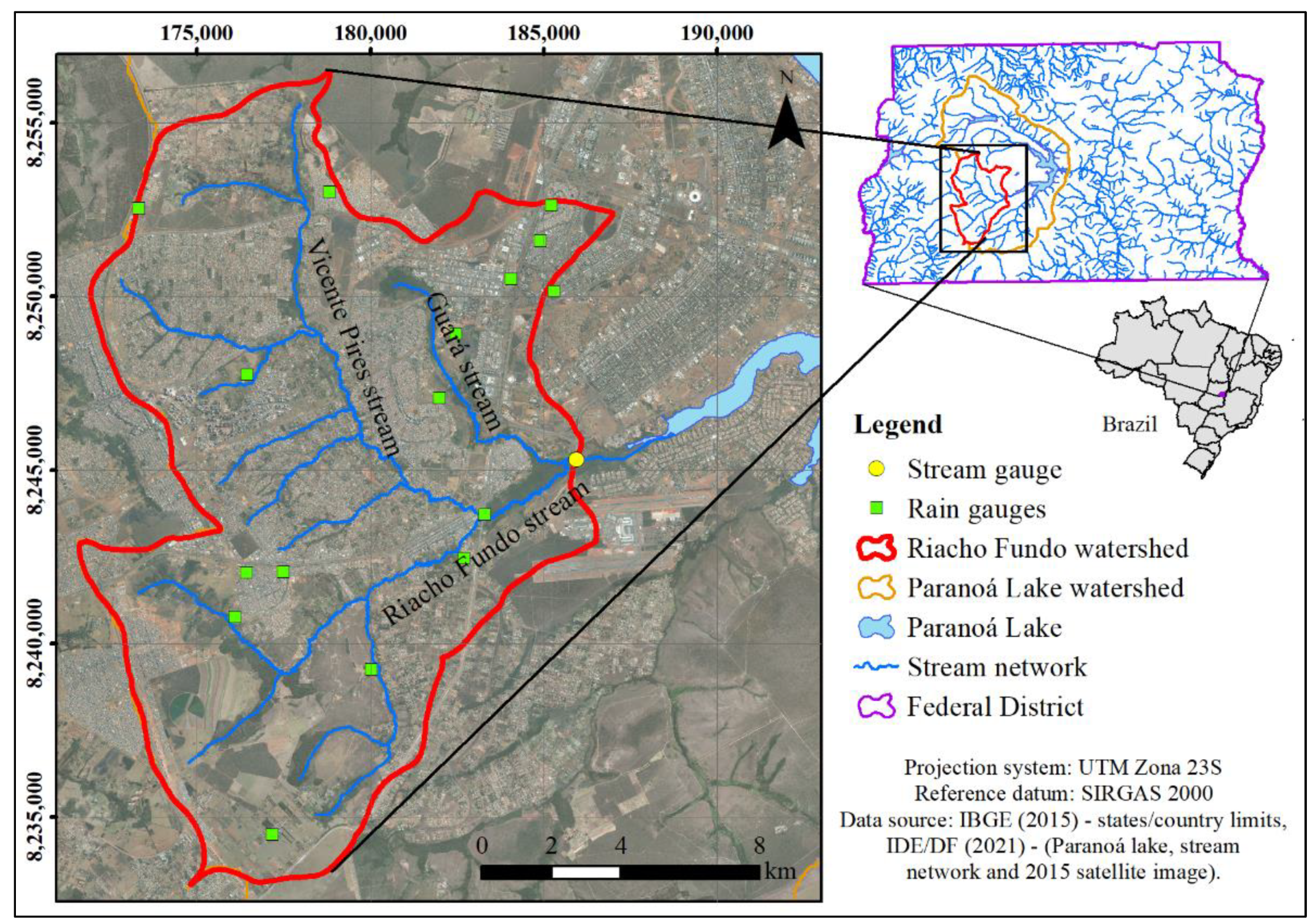
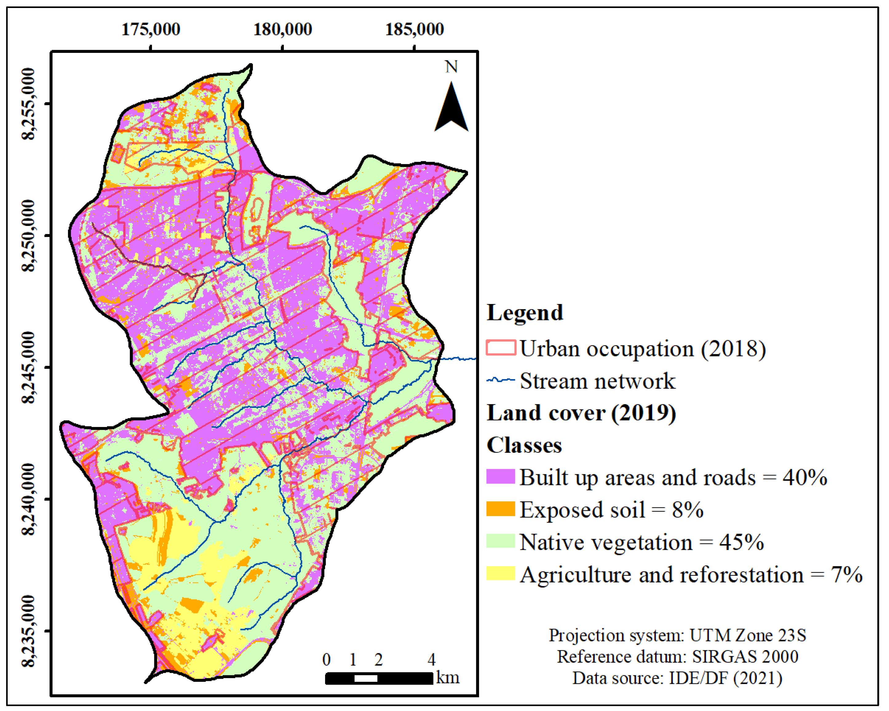
2.1. Study Area

The Riacho Fundo watershed is located in Brasilia, in the Federal District (DF), Brazil, and has an area of 213 km², of which more than 67% are urbanized areas. Paranoá Lake is an artificial reservoir that has four tributary watersheds in addition to the area of direct contribution to it, and the Riacho Fundo watershed, which represents about 21% of the total area of the lake basin, is the one that contributes the most in terms of flow to the water balance of the lake [39]. The Riacho Fundo stream, the main watercourse that gives the watershed its name, is 23.6 km long and receives the streams Vicente Pires and Guará, and two other smaller streams (Figure 1).

The climate in the region is tropical savanna, with well-defined dry and rainy periods. The average annual accumulated precipitation in DF is close to 1500 mm [42], recorded mostly between the months of October and April. The local biome is the Cerrado, with forest, wooded and shrub savannas [43].

Urban occupation in the Riacho Fundo watershed grew rapidly after the 1990s, with the urban area increasing from 26% of the total area of the watershed in 1991 to 62% in 2009, and reaching 67.3% in 2018. The land cover in the watershed, according to the 2019 SENTINEL-2B satellite image classification [44], is composed of approximately 48% nearly impervious areas, corresponding to built-up areas with buildings, roads, and exposed soil. The rest of the area has coverage of native vegetation (45%) and agricultural or reforestation areas (almost 7%) (Figure 2).

The Federal District is located on Brazil’s Central Plateau and in the region of the studied watershed, flat to softly undulating relief prevails, with the average slope of the area being 6.4%. Regarding pedology, there is a predominance of latosols, with red latosol found in 38% of the area and red-yellow latosol in 11.4%, and cambisols, which occupy 21.1% of the area according to the 1978 soil classification [45]. However, the classification does not include soils in urban areas and it is known that urbanization modifies the properties of soils, which makes them complex to survey [46].

According to the 2020 diagnosis of Brazil’s National Sanitation Information System (SNIS), the attendance rates of water supply and sewage collection in the Federal District are 99 and 90%, respectively, and 100% of the collected sewage is treated, while the attendance by household solid waste collection is 98% [47]. In the Riacho Fundo watershed, part of the domestic sewage is directed to individual solutions due to the absence of a collection network, because several occupations are recent. For stormwater, the diagnosis provides an indicator for the attendance of public roads in the urban area by underground drainage network, which in 2020 corresponded to slightly less than half of the roads in the DF [47].

2.2. Diffuse Pollution Monitoring

Rainfall monitoring in the basin included 16 tipping bucket rain gauge stations (Figure 1) and was conducted from October 2019 to April 2021. The stream’s water stage and discharge were monitored at a stream gauging station located near the watershed outflow (Figure 1, station 60478400—Ponte Aeroporto—EPAR 002) from October 2019 to January 2021, using a pressure transducer level logger programmed to collect data every 10 min and discharge-stage rating curves.

The stage (h) versus discharge (Q) rating curve of the stream gauging station for the period October 2019 to July 2020 was developed with data from discharge measurement campaigns with an acoustic profiler and was divided into a section for low (or frequent) discharge, when flow rates were within the banks, and another for high discharge in the occurrence of bank overflow (Figure 3), with extrapolation at unmeasured levels considering the geometry of the section.

The measuring station was relocated to a section approximately 220 m upstream in August 2020 for operational reasons, and the rating curve developed by the company responsible for operating the station for the new section with monthly flow measurements (Equation (1)) was used since it was not possible to conduct discharge measurement campaigns in this section. The contribution from the area between the new and the original section was considered negligible, and it can be assumed that the flow rate for both is equal.

$$\mathrm{Q}=6.313 · {\left(\mathrm{h} - 0.52\right)}^{1.661}$$

(1)

where: Q—discharge (m³/s); h—river stage (m).

Rainfall time series with 5 min intervals were used for data analysis and filling by spatial interpolation by the inverse of the square of the distance. A 10 min interval discharge time series was obtained from the rating curves equations. In periods with missing data from the automatic equipment, daily discharges were calculated by the average of the two daily readings of the staff gauge when available.

Water quality was monitored at the same water stage and discharge monitoring section, with sample collection during 10 flood events from November 2019 to February 2020 and one flood event in December 2020. In the dry period, one sample collection campaign was conducted during a 24 h period in September 2020. An ISCO 3700 automatic sampler, activated by a water level detector fixed in the stream, collected sets of up to 24 water samples per activation at uniform time steps within each event, which ranged from 10 to 20 min for flood events, while in the dry period, the samples were collected at 2 h intervals.

The raw samples were analyzed for the parameters of total solids (TS), suspended solids (TSS), total dissolved solids (TDS), conductivity, turbidity, and chemical oxygen demand (COD), and were also filtered through a 0.7 μm glass fiber filter for nutrient analysis: inorganic nitrogen (Inorg-N), in the forms of nitrite (NO₂⁻), nitrate (NO₃⁻) and ammonia (NH₃), and phosphorus (P), reactive (RP) and total (TP). The methodologies employed (

Table 1. Details of the methodologies used for water quality analysis of the collected samples.

Parameter	Method	Stand. Met. Reference	Equipment	Measuring Range
TS	Gravimetric determination	2540 B	Analytical scale	0.01–210 g
TSS	Gravimetric determination	2540 D	Analytical scale	0.01–210 g
TDS	Differential	-	-	-
Turbidity	Nephelometric	2130 B	Turbidimeter	0–10,000 NTU
Conductivity	Direct measurement	2510 B	Conductivity meter	0.01 μS–200 mS/cm
COD	Reactor digestion, Colorimetric	5220 D	Spectrophotometer, reactor	0–150 mg/L COD (LR) 20–1500 mg/L COD (HR)
NO2−	Diazotization, Colorimetric	4500-NO2 B	Spectrophotometer	0–0.3 mg/L NO2-N
NO3−	Cadmium reduction, Colorimetric	4500-NO3 E	Spectrophotometer	0–0.5 mg/L NO2 + NO3-N (LR) 0–5 mg/L NO2 + NO3-N (MR)
NH3	Nesslerization, Colorimetric	4500-NH3 C (1995)	Spectrophotometer	0–2.5 mg/L NH3-N
RP	Ascorbic acid, Colorimetric	4500-P E	Spectrophotometer	0–2.5 mg/L PO43−
TP	Acid persulfate digestion, Colorimetric	4500-P B 4500-P E	Spectrophotometer, reactor	0–3.5 mg/L PO43− 0–1.1 mg/L P

LR—low range; MR—medium range; HR—high range.

) followed the Standard Methods For The Examination Of Water And Wastewater [48] as reference.

2.3. Water Quality Assessment

The extent of the impact of pollutant concentrations depends on the volumes associated with them. Thus, pollutant loads, which represent pollutant discharge rates, are an important measure for assessing water quality [8]. From the concentrations determined in the samples, the pollutant loading rates at a given time (W) were calculated by multiplication between concentrations (C) and flow rates (Q) using the unit of tons/day (Equation (2)) and plotted against the flow rates for graphical analysis of the distribution of points.

$$\mathrm{W}=\mathrm{C} · \mathrm{Q} · \mathrm{k}$$

(2)

where: W—pollutant loading rate (ton/day); C—pollutant concentration (mg/L); Q—flow rate (m³/s); k—constant for unit conversion (k = 0.0864 for the units presented).

The cumulative pollutant load (L) over a period can be obtained by adding load rates at shorter intervals (Equation (3)), which was carried out for each event. The pollutant load rates (W) representing each time interval (∆t) were summed and the appropriate unit conversion was performed. Dividing the event’s pollutant load by the accumulated water volume, the event mean concentration (EMC) was also calculated (Equation (4)). This is an important indicator to assess the impact on the water quality of receiving bodies, which present variation in pollutant concentrations due to stormwater discharge, but with a slightly slower response [49]. In addition, the EMC has a distribution characteristic that facilitates the interpretation and comparison of results between different areas and events [50] and has already been applied for this purpose in several research studies on surface runoff [10,51-53] and watercourses [12,54,55].

$$\mathrm{L}=\mathrm{k} ·\int \mathrm{C}\left(\mathrm{t}\right) · \mathrm{Q}\left(\mathrm{t}\right) \mathrm{dt}=\mathrm{k} ·{\displaystyle \sum }_{\mathrm{i}=1}^{\mathrm{n}}{\mathrm{C}}_{\mathrm{i}} ·{ \mathrm{Q}}_{\mathrm{i}} · \Delta \mathrm{t}$$

(3)

where: L—cumulative load over a period (ton); C_i—pollutant concentration at instant i (mg/L); Q_i—flow rate at instant i (m³/s); ∆t—represented time interval (min); k—constant for unit conversion (k = 6 ∙ 10⁻⁵ for the units presented).

$$\mathrm{EMC}=\frac{\mathrm{L}}{\mathrm{V}}=\frac{\int \mathrm{C}\left(\mathrm{t}\right) · \mathrm{Q}\left(\mathrm{t}\right) \mathrm{dt}}{\int \mathrm{Q}\left(\mathrm{t}\right) \mathrm{dt}}\cong \frac{{{\displaystyle \sum }}_{\mathrm{i}=1}^{\mathrm{n}}{\mathrm{C}}_{\mathrm{i}} ·{ \mathrm{Q}}_{\mathrm{i}} · \Delta \mathrm{t}}{{{\displaystyle \sum }}_{\mathrm{i}=1}^{\mathrm{n}}{\mathrm{Q}}_{\mathrm{i}} · \Delta \mathrm{t}}$$

(4)

where: EMC—event mean concentration (mg/L); L—pollutant load of the event; V—discharge volume of the event; C_i—pollutant concentration at instant i (mg/L); Q_i—flow rate at instant i (m³/s); ∆t—represented time interval (min).

For each water quality monitoring event, precipitation in the total watershed area and the observed flood wave at the outfall were characterized by the monitoring data. In determining the characteristics of precipitation volume, duration, and intensity, all monitoring stations in operation for each event and all records contributing to the flood wave were considered. For counting the number of antecedent dry days (ADD) a threshold of 1 mm was established, equivalent to the initial abstraction of impervious areas in the SCS method for quantifying runoff. The justification for this is that the watershed is highly urbanized and has impervious areas spread throughout its entire extent, therefore precipitation volumes above this would generate runoff. The inverse distance squared method was used to prepare maps of the spatial distribution of the events’ total precipitation volume, and the coefficient of variation around the mean was calculated for each. Finally, the flood wave was characterized by its flow rates and duration.

Pearson’s correlation coefficients (r) were calculated for the hydrologic characteristics among themselves and with the EMCs. Possible connections between the area of rainfall concentration and the response in the stream’s water quality were investigated by analyzing the EMCs along with the rainfall spatial distribution maps.

2.4. Comparison of Methodologies for Estimating Long-Term Pollutant Loads

In order to estimate the pollutant loads in unmonitored periods, rating curves relating flow rates to pollutant loads measured for the collected samples were fitted. The parameters TSS, Inorg-N, TP, and COD were chosen for the elaboration of the curves because they were considered to provide a general representation of the behavior of the concentrations of solids, the main nutrients, and organic matter in the stream. A simple regression process between loading and flow rates was employed using a non-linear model and optimizing the parameters, following the methodology used by Menezes et al. [56].

Like the discharge-stage rating curve, the pollutant rating curves were plotted for two flow rate ranges. For low discharges, non-linear regression was applied to the observed data using the best-fit curve type based on a preliminary analysis. The fit was forced to the dry period flow rates since due to limitations caused by the COVID-19 pandemic it was not possible to obtain many measurements in the period, and the parameters of the curve equations were optimized by minimizing the sum of squared errors. Data from the event on 5 December 2020 were not used in the fitting of the rating curves as it was assessed that the change of section of the stream gauging station could imply errors. Thus, for high discharges, the data observed in only one event (24 February 2020) were considered to perform the regression and obtain the rating curve. For the water quality parameters whose loads presented hysteresis behavior, the rating curve was plotted as an average curve between the curves generated by regressions in the ascending and descending limbs of the flood wave, aiming to produce a compensation effect in the estimation of accumulated load values, with underestimation of values from the upper curve and overestimation of those from the lower curve.

The evaluation of the fits of the pollutant rating curves was carried out by calculating the coefficient of determination (R²), the standard error of the estimate (S), and the ratio between observed and estimated loading rates. Furthermore, the accumulated pollutant loads in the monitored events were estimated by the rating curves and the same metrics were calculated again, with the addition of the Nash–Sutcliffe model efficiency (NSE).

The accumulated monthly and annual pollutant loads were estimated from two methodologies: the first one using the pollutant rating curves to estimate the load rates continuously based on the 10-min interval flow series, and the second one adopting a monthly concentration measurement to calculate pollutant loads by multiplying it with average daily flows obtained by two daily stream stage records. This latter methodology is equivalent to the one currently used by the local institution that performs the monthly water quality monitoring in the Riacho Fundo stream.

For a proper comparison, both estimates used data from the monitoring performed in this work. To simulate the monthly concentration measurement, the pollutant concentrations on a fixed day and time each month were calculated based on the load rate observed at the time calculated by the pollutant rating curves, and the two daily water stage readings, also needed for the second methodology, were extracted from the continuous monitoring by fixing times for them, one in the morning and one in the afternoon. After calculating the pollutant loads, at 10 min intervals in the first methodology (rating curves) and 1-day intervals in the second methodology (monthly monitoring), they were accumulated to estimate the monthly and annual pollution loads and then compared to each other in terms of order of magnitude and percentages. The pollutant loads estimated by the rating curves methodology were also compared to load values found in the literature and analyzed as to the contribution portion of each season in a hydrological year.

3. Results and Discussion

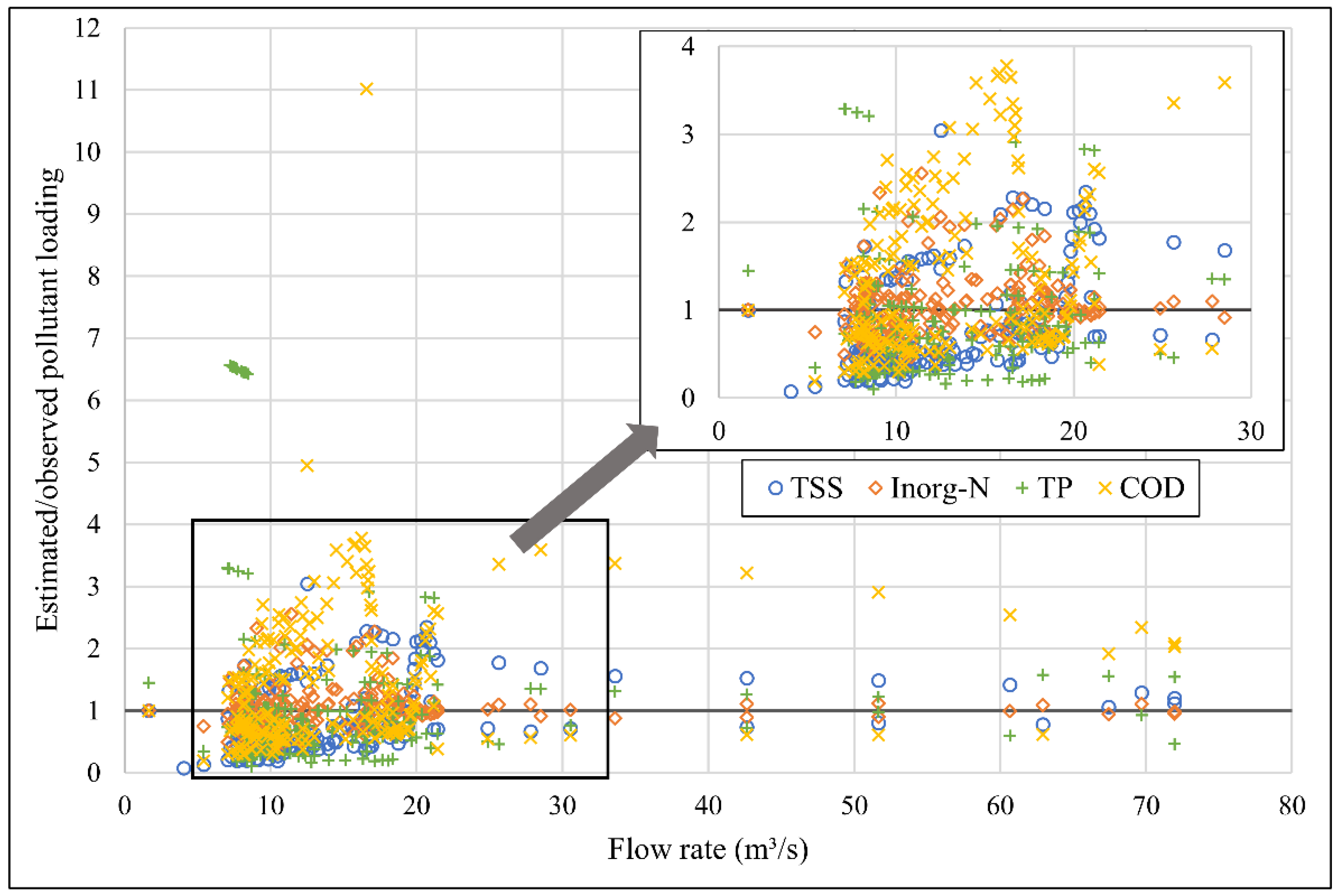
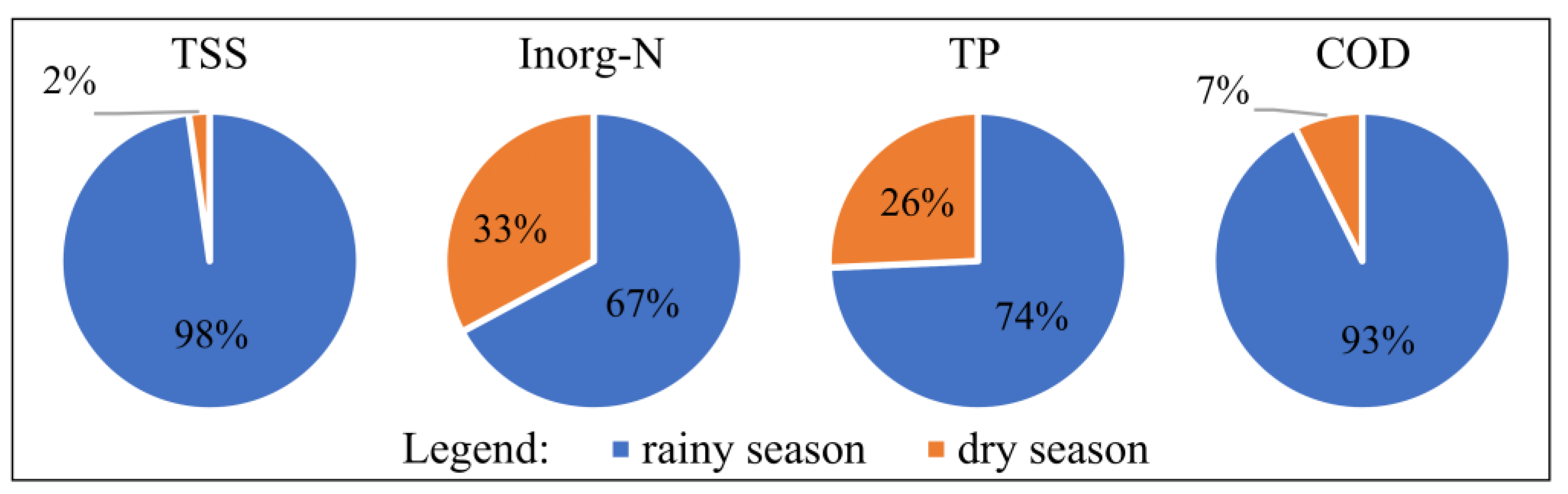
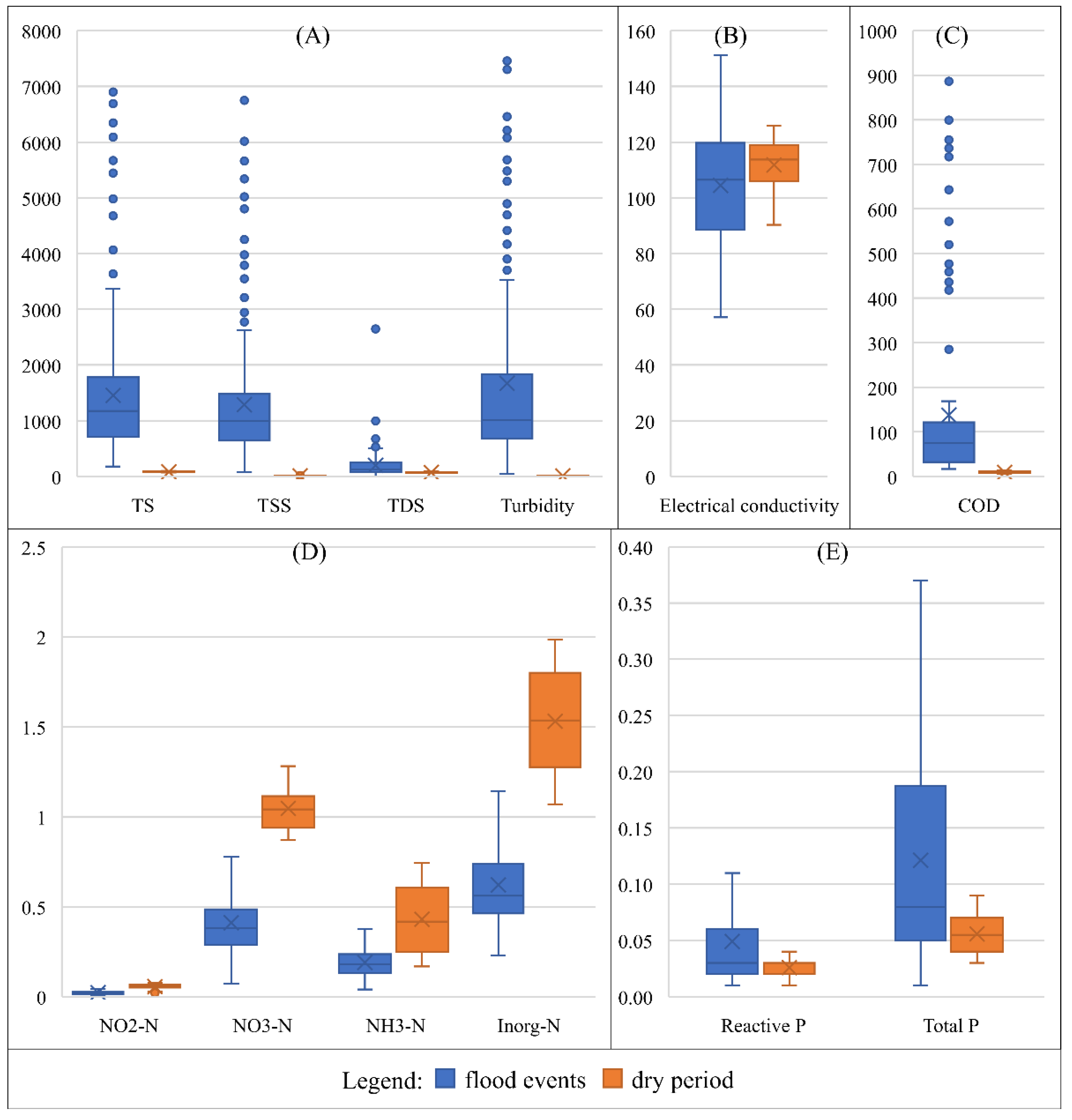
3.1. Collected Data and the Effects of Diffuse Pollution on Water Quality

The highest 5 min precipitation rate observed in the monitored period was 182.4 mm/h. Cumulative monthly precipitation was also calculated to analyze trends. Variations were observed from −75% to +146% from the historical monthly averages, however, in most months the accumulated rainfall did not vary more than 30% from the average. The average total annual precipitation among the stations was 1282 mm for the 2019–2020 hydrological year (October to April) and 1388.5 mm for the year 2020, values respectively 14 and 7% lower than the historical average of 1493 mm [42]. Nevertheless, analysis of the rainfall data obtained from monitoring and historical data indicated that these were not atypical years in terms of precipitation.

The flow rates at the gauging station varied between 1 and 99 m³/s during the monitored period, as the stream stage ranged between 0.54 and 3.39 m. Discharges consistent with stream bank overflow were observed in only eight rainfall-runoff events between October 2019 and July 2020, the period in which monitoring was conducted in the original section.

A set of seven to 41 samples was collected per event, depending on its magnitude and on the operation of the autosampler. The flood wave was fully monitored, with proper automatic activation and deactivation by level detection, in seven events, and sampling occurred during the rise and depletion of the wave, including the peak, in nine of the 11 events, in which it is considered that a representative set of samples of the water quality was obtained. Two events only had samples collected at the rise of the flood wave (also including the peak flow), and these were 5 December 2019 and 5 December 2020. Sampling in flood events occurred at flow rates from 7 to 72 m³/s.

Sampling in the dry period was performed on 18 Sep. 2020, when the drought had already lasted about 118 days. The average flow observed in the Riacho Fundo stream during the 24 h of the sample collection was 1.65 m³/s, with a variation of less than 0.2 m³/s. This flow rate is close to the lowest observed in the stream during the monitoring period and in historical data of monthly minimum flows [57].

The mean, maximum and minimum pollutant concentrations were calculated and compared between the flood events and the dry period. The representation of the pollutant concentrations in boxplots shows the variation that occurs between these occasions, which in the case of turbidity and the concentrations of total and suspended solids and COD corresponds to the significant increase during flood events (Figure 4) linked to the contribution of surface runoff and bank erosion.

Nitrogen concentration, on the other hand, is higher during the dry season (Figure 4), which indicates that continuous discharges of domestic sewage into the watercourses of the watershed are possibly its main source. As nitrate is the form that presents the highest concentrations in both periods and a more expressive increase in low flow conditions, these discharges are older, a situation compatible with the effluent from the sewage treatment plant present in the basin, or are made at points further upstream. In flood events, high discharges cause the dilution of this pollutant.

Phosphorus concentrations are low in the Riacho Fundo stream, often resulting in values close to the detection limit of the method used, which leads to small differences between drought and flood events (Figure 4). It is known that phosphorus can be transported along with the suspended solids and that the sediment is the main P storage compartment in Paranoá Lake [58], which may be the cause of the low detection of this parameter dissolved in the water, although to a lesser extent, an increase in the concentrations of this parameter is observed due to diffuse pollution.

Analyzing the loads corresponding to the concentrations obtained (Figures S1–S4), it can be seen that there was a clear occurrence of hysteresis phenomenon at very high flows, observed in the two events that overflowed the stream banks, for the parameters suspended and total solids and COD, with higher loads occurring at the rise of the flood wave. For nitrogen and total phosphorus, even though there was a difference in loads of the rising and depleting flood wave, the phenomenon was not very pronounced, and for reactive phosphorus, no hysteresis was identified. At lower flows, observed within the stream banks, hysteretic behavior could be observed in most events for solids and in some events for nitrogen and COD parameters, mostly with higher loads during the depletion of the flood wave. This behavior was also found for TSS in a study performed in another section of the Riacho Fundo stream [59].

The EMC values varied greatly between the rainy and dry seasons (

Table 2. EMCs in the events monitored at the stream gauging station in mg/L.

Event	COD	TS	TSS	NO2-N	NO3-N	NH3-N	Inorg-N	RP	TP
7 November 2019	95	932	806	0.02	0.28	0.26	0.56	0.05	0.28
5 December 2019 *	98	1664	1258	0.01	0.25	0.15	0.41	0.03	0.07
18 December 2019	35	1130	989	0.02	0.34	0.18	0.54	0.03	0.09
22 December 2019	23	1040	899	0.02	0.63	0.09	0.73	0.05	0.07
23 December 2019	25	1681	1363	0.03	0.35	0.17	0.54	0.03	0.07
10 January 2020	96	1053	1053	0.05	0.70	0.19	0.94	0.02	0.09
23 January 2020	58	515	413	0.04	0.18	0.23	0.46	0.08	0.01
30 January 2020	29	267	178	0.02	0.57	0.16	0.75	0.02	0.01
23 February 2020	51	451	120	0.02	0.45	0.09	0.56	0.07	0.05
24 February 2020	171	1472	1360	0.01	0.35	0.17	0.53	0.07	0.06
5 December 2020 *	534	3775	3530	0.03	0.62	0.27	0.91	0.07	0.21
Mean	110	1271	1088	0.02	0.43	0.18	0.63	0.05	0.09
Median	58	1053	989	0.02	0.35	0.17	0.56	0.05	0.06
Minimum	23	267	120	0.01	0.18	0.09	0.41	0.02	0.01
Maximum	534	3775	3530	0.05	0.70	0.27	0.94	0.08	0.21
Dry period	9	82	11	0.06	1.04	0.43	1.53	0.03	0.06

* Sample collection only at the rise of the flood wave.

), following the concentration characteristics already discussed for each pollutant. Between flood events, there was also variation in EMCs.

The concentrations and EMCs of solids found in flood events in the Riacho Fundo stream are significantly higher than those found in runoff from urbanized areas collected by drainage networks in an absolute separator system [9,10,51], including that from residential areas within the studied watershed [11,40,60]. Regarding nitrogen, nitrate stands out, and its observed concentrations and EMCs were higher in the stream than in the runoff from these areas [9,11,40]. Phosphorus EMCs in the stream, on the other hand, were found to be lower than those in surface runoff. Finally, COD concentrations and EMCs found in the stream were often much higher than those that have been determined for runoff from urban areas, coming closest only to the EMCs found in areas outside the watershed [10,51].

In comparison to other watercourses, the Riacho Fundo stream has turbidity, and both point and EMCs of solids and COD were much higher than those in natural [18,61] or rural watersheds with little urban occupation [12,15,62,63]. More preserved watersheds or those with predominantly rural use show ammonium ion concentrations higher than those of the Riacho Fundo stream [18] and similar EMCs [15]. The high input of organic material and the use of fertilizers are factors that lead to increased ammoniacal nitrogen in water bodies and, therefore, may justify the proximity of the concentrations in these areas to those found in this study. Phosphorus EMCs in the rural watershed studied by Kozak et al. [15] were also low and close to those found in the Riacho Fundo watershed.

Watersheds considered urban or with mixed land use, having a significant percentage of urbanized areas, present concentrations and EMCs of suspended solids and turbidity in flood events many times close to or higher than those of the Riacho Fundo stream [12,13,16], and the difference depends on the proportions of the watershed. Nitrogen concentrations found in these types of watersheds are also closer to or slightly higher than those observed in the Riacho Fundo stream, both in flood events and in the dry period [16,64,65]. Phosphorus concentrations in flood events in the Riacho Fundo stream were lower than those found in smaller urban watersheds [64,65], but higher than those found in a larger watershed [16], an observation that may be linked to the potential for diluting concentrations of this pollutant. Both lower [65] and higher [13] COD concentrations than those found in the Riacho Fundo watershed were observed in other urban watersheds, reinforcing the hypothesis that the higher the degree of urbanization, the higher concentrations of this pollutant.

In the Vicente Pires stream, a tributary of the Riacho Fundo stream that drains a highly urbanized area, Costa et al. [20] found pollutant concentrations very close to those found in this study. On average, concentrations at flood events in the Vicente Pires stream were slightly lower for nitrogen forms and somewhat higher for turbidity, phosphorus, and COD than those in the Riacho Fundo stream, indicating that this tributary is a major contributor of high pollutant loads to the studied watershed. Even with higher water discharges, the concentrations of pollutants in the watershed outfall are not attenuated, an observation that leads to the conclusion that other tributaries and the areas adjacent to the Riacho Fundo stream itself also contribute to the deterioration of the quality of the stream’s water. In the dry period, the mean concentrations analyzed in the streams Vicente Pires and Riacho Fundo are also similar, but Costa et al. [20] monitored more events, in different months, and therefore found a wider variety of concentrations for this period, a behavior that should also be observed in the Riacho Fundo stream.

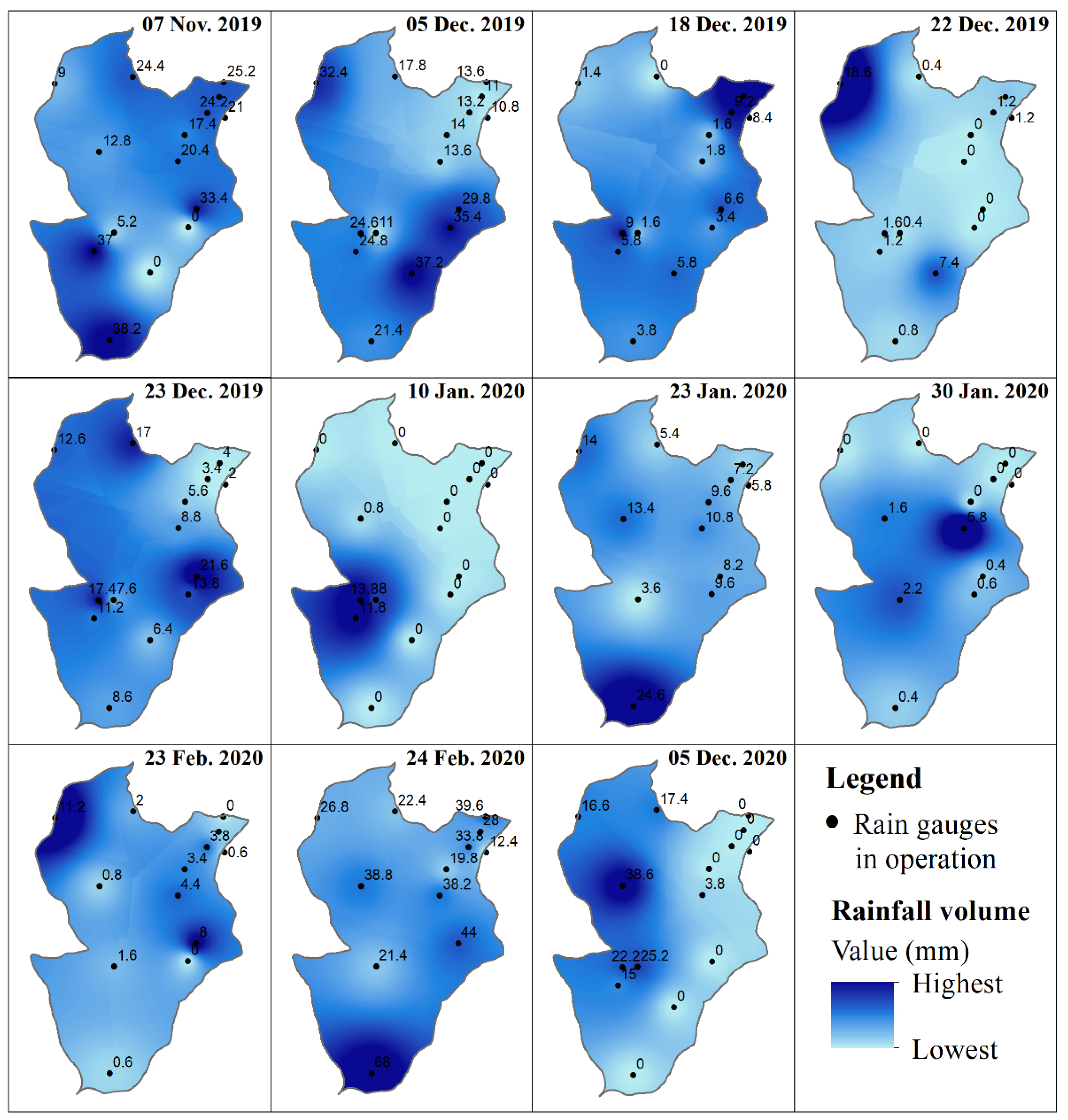
3.2. Water Quality Correlation with Hydrological Characteristics and Rainfall Spatial Distribution

There was great variability in precipitation volumes, durations, and intensities among the events, which also produced floods of different magnitudes (

Table 3. Rainfall and flood characteristics associated with monitored events in the Riacho Fundo watershed.

Event	Mean * Cumulative Volume (mm)	Mean * Duration (min)	Mean * Intensity (mm/h)	Mean * ADD (Days)	Mean Flow Rate (m3/s)	Max Flow Rate (m3/s)	Flood Duration (Hours)
7 November 2019	22.5	105	13.7	0.5	11.5	19.3	14.7
5 December 2019	20.7	575	2.2	0.6	11.7	18.8	22.7
18 December 2019	5.8	98	7.8	2.3	8.3	14.0	8
22 December 2019	3.5	19	11.1	2	6.3	9.9	7.3
23 December 2019	10	95	8.4	1.5	11.0	16.9	10.7
10 January 2020	8.6	11	42.4	0	8.4	11.0	5.5
23 January 2020	9.8	462	1.3	0.4	6.2	8.3	14.5
30 January 2020	1.8	56	6.9	0.7	7.2	8.5	5.8
23 February 2020	3.4	59	4.4	0.9	8.1	10.6	4.3
24 February 2020	32.8	375	5.6	0.3	25.0	71.9	20.5
5 December 2020	17.6	42	32.3	10.8	21.0	32.1	10.5

* Arithmetic mean among the stations that recorded volume > 0 mm for the events.

). The event with the highest precipitation volume was the one that reached maximum flow rate, and these two variables showed a strong positive correlation (r = +0.83), as expected. In addition, not surprisingly, longer precipitation durations were associated with longer flood wave durations (r = +0.86). Rainfall intensity and the number of antecedent dry days (ADD) showed, in general, weak correlations with flood characteristics (Table S1).

Events with lower magnitude floods presented, in general, lower EMCs for solids and COD, but are associated with higher EMCs for nitrogen, especially nitrate, while events with higher flow rates present opposite behavior for these concentrations. The strongest correlation found between EMCs and mean flow rate was for TSS, TS, and COD, with coefficients close to +0.7, higher than any correlation found by Park et al. [65] for the same parameters in watersheds with predominantly forest and agricultural land cover. Costa et al. [66] found a strong correlation between these pollutants and peak flow for the Vicente Pires watershed, a tributary of the Riacho Fundo stream, although at Riacho Fundo stream the TSS, TS, and COD EMCs correlations with maximum flow rate were moderate (r ≈ +0.4).

NO₃-N EMCs were most strongly correlated with the flood duration characteristic (r = −0.67), and were inversely proportional to all flood characteristics, as were the EMCs for NO₂-N and Inorg-N. This is due to dilution caused by large discharge volumes, also observed by Girardi et al. [18] for a natural land cover watershed.

Precipitation characteristics also influenced the pollutant concentrations and loads observed in the stream. Higher precipitation intensities and a higher number of ADDs were observed in the events of higher instantaneous loads and EMCs for solids and COD, an observation that somewhat extends to the loads and EMCs of nitrate nitrogen, the predominant form of inorganic nitrogen in the stream. The positive correlation of the EMCs of TS, TSS, and COD is stronger concerning the mean ADD (r between +0.86 and 0.88) than the mean precipitation intensity (r between +0.46 and 0.53) and accumulated volume (r = +0.43 for all of them). Brites and Gastaldini [12] found a positive correlation between suspended solids and the mean intensity and total volume of precipitation in the watershed, but not with the previous dry period. The authors emphasized that the correlations with precipitation characteristics vary among different parameters. Costa et al. [41] did not identify any strong correlation between TSS EMCs and rainfall characteristics, being the highest correlation coefficient the one with precipitation volume, reinforcing the conclusion that in addition to varying among different pollutants, correlations with hydrological characteristics vary with other factors such as characteristics of the watershed, which was also pointed out by Perera et al. [53].

The NO₃-N and Inorg-N EMCs, on the other hand, correlate more strongly with mean precipitation intensity (r = +0.72 and +0.87, respectively) than with ADD (r = +0.36 and +0.49). Higher precipitation intensities generate higher EMCs in runoff as they can mobilize more pollutants at the surface, and the number of preceding dry days also has a significant contribution since it is related to the accumulation of these pollutants [53]. These parameters also correlate negatively with mean rainfall volume (r < −0.2) and duration (r < −0.7), probably because of the relationship with increased flow rates. It is a divergent behavior from that found by Costa et al. [41] for the nitrate and ammonia EMCs in the Vicente Pires stream within the Riacho Fundo watershed, which were higher the greater the rainfall volumes. Thus, it is assumed that the rainfall incident in the highly urbanized Vicente Pires watershed carries a major portion of the nitrogen pollution to the Riacho Fundo stream.

It was not possible to clearly identify event characteristics that influenced the values of instantaneous loads and phosphorus EMCs, which did not show a strong correlation with any of the analyzed characteristics. The low concentration values and small variation of this pollutant between events may have contributed to the lack of correlations with precipitation and flow rates, but for other hydrological variables, the correlation may be more expressive. For total runoff volume, Costa et al. [41] found a strong positive correlation with EMCs for reactive and total phosphorus. Mallin et al. [67] evaluated cumulative rainfall in the 72 h before the event and also found a positive correlation with total phosphorus.

The spatial distribution of the total precipitated volume in the events (Figure 5) indicated varied behaviors not only between different events, but also within them, illustrating the variability of rainfall. The lowest coefficient of variation of the total precipitation volumes at the rainfall stations for an event was 0.4 while the highest was 2.1, and in five of the events, the coefficient was above 1, indicating that the standard deviation obtained a value greater than the mean among the precipitation volumes. A more heterogeneous distribution is expected in events with higher coefficients of variation.

From the maps, it was possible to make some remarks regarding the approximate areas of the greatest concentration of precipitation in each event. The concentration of higher precipitation volumes in the southern part of the basin, where there are more preserved areas or areas with rural use, was observed in common events (with flows within the stream channel) that presented higher EMCs of ammoniacal nitrogen, but lower EMCs of nitrate (7 November 2019 and 23 January 2020). In the events where rainfall was concentrated mainly in urbanized areas (22 December 2019, 10 January 2020, and 23 February 2020), the EMCs of NO₃-N were the highest and of NH₃-N the lowest. The lowest EMCs of COD occurred in the events that had concentrated rainfall in more urban areas (22 December 2019, 23 December 2020, and 30 January 2020) and the highest were found in events with concentrated rainfall in both more rural (7 November 2019) and more urban areas (10 January 2020).

These findings lead to the belief that the main sources of ammonia concentrations for the Riacho Fundo stream are agricultural activity and natural areas, probably due to the input of organic material and, possibly, fertilizers. Works that evaluated biochemical oxygen demand (BOD) in the water of different streams [12,50,66,67] found the opposite: urban areas contributed more to higher organic matter, as did Chen et al. [14], who specifically found higher ammonia contributions from urban areas than from rural ones. However, differences in the sewage collection system and raw sewage amount and discharge points may have led to this divergence, as it is known that higher ammonia concentrations are linked to raw and recent sewage; in the Riacho Fundo basin there is the discharge of treated effluent and raw sewage discharges are probably made at points upstream of the monitoring section.

Although no similarity was identified between the spatial distributions of rainfall in the events of lower solids EMCs, in all smaller-scale events associated with the high EMCs of these pollutants (>1000 mg TS/L and >900 mg TSS/L) there is the incidence of rainfall over some urbanized area. Brites and Gastaldini [12] also found higher suspended solids EMCs from a more urbanized watershed, compared to a less urbanized one, just as Mallin et al. [67] indicated that an urban stream yielded higher TSS concentrations than suburban and rural ones. The EMCs of solids found by Choi et al. [52] for areas with an urban occupation were high, but still not high enough to state that these areas are the largest contributors to high concentrations of this pollutant, highlighting the EMCs from field areas.

Once again, the phosphorus EMCs could not be related to any spatial distribution characteristics of the rainfall. Nevertheless, in events of greater magnitude, in which discharges that exceeded the stream channel were observed, EMCs of almost all pollutants, especially COD, TS, and TSS, were much higher when the rainfall was concentrated in the urban area (5 December 2020) than when it was concentrated more in the rural part of the basin (24 February 2020). This observation may be linked to the fact that, in the event of 5 December 2020, only the rising limb of the flood wave was monitored for water quality, not computing the complete behavior of the concentrations of pollutants which, as previously discussed, presents hysteresis for some of them. However, as concluded from the other events, it appears that the areas with urban occupation in the Riacho Fundo watershed are the main sources of pollution for this stream.

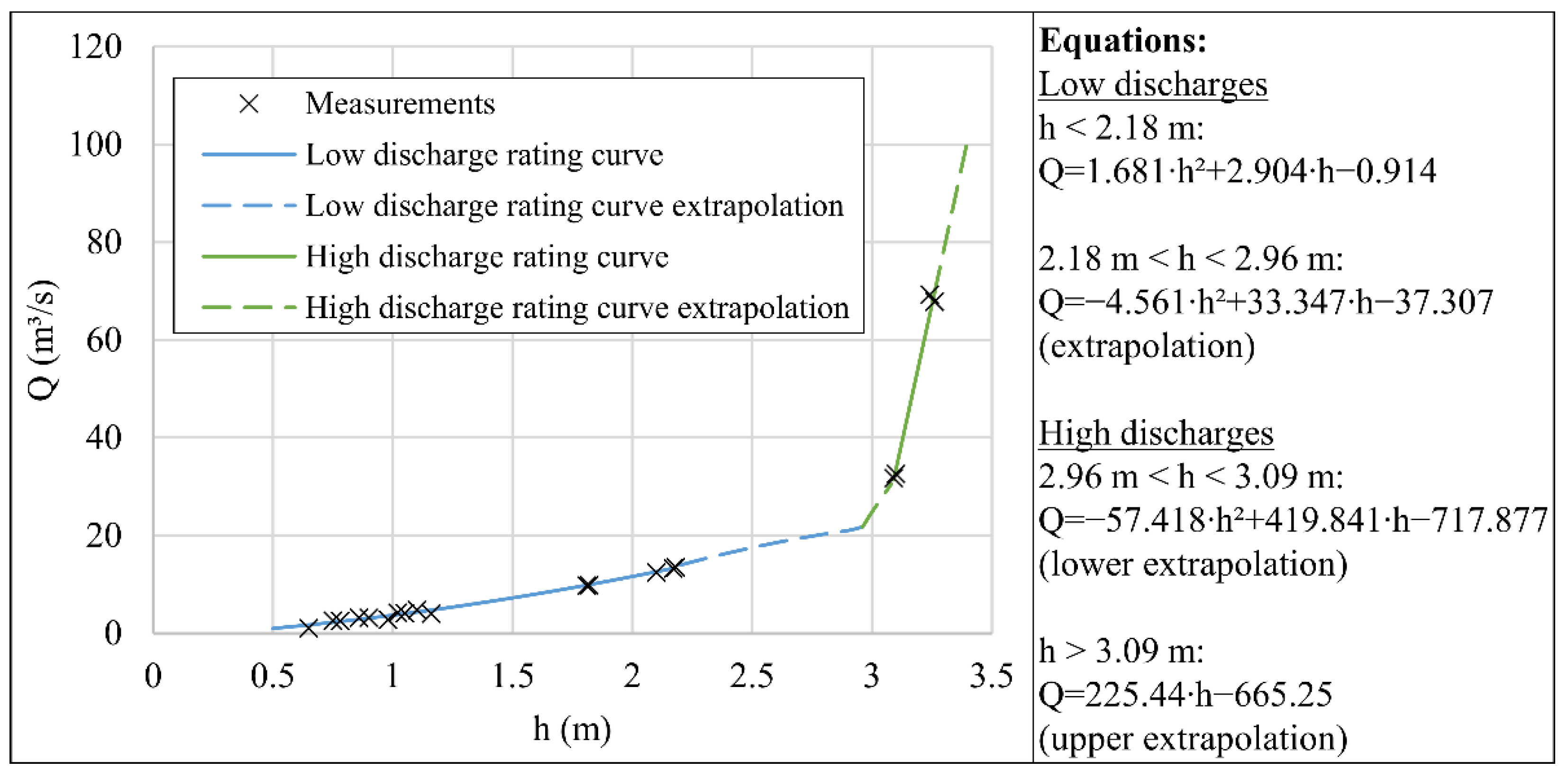
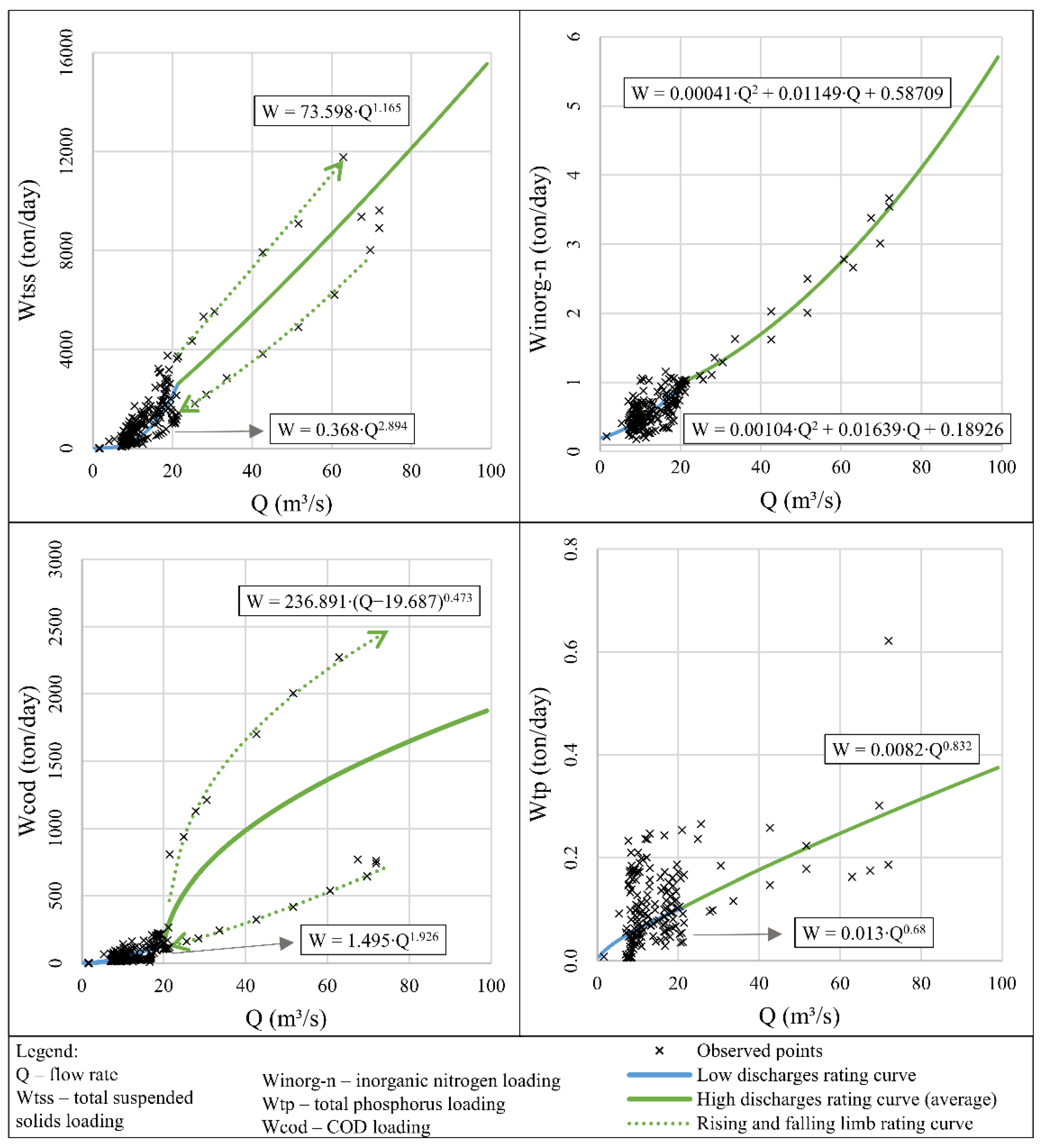
3.3. Pollutant Rating Curves

The rating curve fitting resulted in power equations for the suspended solids, total phosphorus and COD parameters, and polynomial for the inorganic nitrogen parameter (Figure 6). The intersection between the low and high discharge curves occurs at a flow rate of 21.4 m³/s for TSS, Inorg-N, and TP and 20.1 m³/s for COD.

The metrics calculated for the fits are suitable for evaluating the pollutant rating curve only for the low discharges (less than 21.4 m³/s), at which there are more points observed and at different events. As this discharge range occurs in the stream much more frequently, it is more important that the curves fit it and therefore the discussion was restricted to these discharges. The resulting R² coefficients indicated challenges in fitting the curves (

Table 4. Metrics for pollutant rating curves fitting.

Pollutant Rating Curve		R2	S (ton/Day)
TSS	Low discharges	0.51	482.37
	High discharges	0.68	1760.36
Inorganic N	Low discharges	0.38	0.15
	High discharges	0.97	0.18
Total P	Low discharges	0.06	0.02
	High discharges	0.28	0.06
COD	Low discharges	0.43	31.47
	High discharges	0.3	430.7

), with the highest value being 0.51 for the TSS rating curve fit. The fits of the Inorg-N and COD rating curves obtained slightly lower R², 0.38 and 0.43, respectively, and the TP rating curve, in contrast, obtained the worst fit, with an R² of 0.06. It can be stated that the R² values were impacted by the forced fit to the data obtained in the dry season and the continuity constraint between the curves for high and low discharges; however, the observed data also naturally showed some dispersion. The TP loading rates especially were associated with high dispersion, showing a low correlation with the flow rate, and making it difficult to achieve a good fit.

Evaluating the standard error of the regression is important since the fitting followed a nonlinear model. In general, all parameters except TP had standard errors of a smaller order of magnitude than most of their loading rate values. The TSS rating curve had the largest absolute value of standard error; in proportion to the loading rates, however, it is of little significance. Although it showed a lower standard error, the TP rating curve had more significant divergence when analyzed with the low loading rates of this pollutant.

By analyzing the ratios between estimated and observed pollutant load rates (Figure 7), it can be seen that the TSS and TP rating curves, despite overestimating the loading rates in comparison with those observed in some situations, presented the tendency to underestimate the loading rates at low discharges, which is proven by the median of the ratios, of 0.60 and 0.77 for each respectively. For TSS, a possibly larger number of samples collected during the rise of the flood wave may have influenced the tendency of the rating curve, since the hysteresis phenomenon was identified for this parameter. For the Inorg-N and COD rating curves no clear trend was identified, with approximately half of the observations having been overestimated and half underestimated, to a greater or lesser degree. The Inorg-N loading rates were the ones that presented the mean and median of the ratio between observed and calculated values closest to 1, indicating that this pollutant’s curve approximated well to the mean of the data obtained in the field and compensated better for the variations in pollutant loading.

The estimation of the total loads transported in the events by the pollutant rating curves resulted in values, in general, of the same order of magnitude as those observed (

Table 5. Total cumulative loads in the events observed and estimated by the pollutant rating curves.

Event’s Total Pollutant Load	TSS (ton/Event)		Inorg N (kg/Event)		Total P (kg/Event)		COD (ton/Event)
	Obs.	Estim.	Obs.	Estim.	Obs.	Estim.	Obs.	Estim.
7 November 2019	165.8	106	116	108.5	57.2	12.7	19.5	11.5
5 December 2019	236.8	174.3	77.9	97.7	20.1	11	18.4	14.3
18 December 2019	151.8	70.2	82.4	79.5	14.4	9.4	5.3	8.3
22 December 2019	52.6	17.1	42.9	31.2	4.3	3.7	1.3	2.6
23 December 2019	427.2	229.1	170.2	161.1	21	18.6	7.7	21.3
10 January 2020	134.4	37.8	117.1	67.4	11.6	8	12.2	5.6
23 January 2020	25.5	13.3	28.4	34.7	0.8	4	3.6	2.4
30 January 2020	15.3	19.2	64	47.7	1.1	5.6	2.5	3.3
23 February 2020	43.5	27.8	54.5	52	4.9	6.1	5	4.2
24 February 2020	2192.8	2027.2	793.8	790.8	89.4	78.2	254.2	301.8
5 December 2020	1362.4	530.7	351.8	196.3	80.3	21.2	206	86.2

), but mostly underestimated (Figure 8). However, the fitted curves showed good performance in estimating event pollutant loads by the calculated metrics (

Table 6. Metrics for the estimation of total event loads.

Total Event Pollutant Load Estimate	R2	NSE	S
TSS	0.89	0.84	194.9 ton/event
Inorganic N	0.95	0.95	46.9 kg/event
Total P	0.6	0.47	13.6 kg/event
COD	0.81	0.8	39.3 ton/event

), with R² and NSE greater than 0.8 for TSS, Inorg-N, and COD, and rather lower for TP, 0.6 and 0.47, respectively. TP presented greater differences in the ratio between estimated and observed total accumulated load, again due to the load values found in the Riacho Fundo stream being very low for this parameter, which makes small differences quite expressive. The pollutant load compensation effect in high discharges intended by employing the average rating curve for the TSS and COD parameters that present hysteresis was achieved in the event on 24 February 2020, which had discharges in the highest range and the lowest ratio between the estimated and observed load for TSS and the second-lowest for COD. The event on 5 December 2020, despite having high discharges, only had samples collected at the rise of the flood wave, and it was not possible to verify this effect.

Moriasi et al. [68] indicate as very good performance for simulations at the watershed scale and monthly step R² > 0.85 and NSE > 0.8 for sediment, R² >0.7 and NSE > 0.65 for nitrogen, and R² > 0.8 and NSE > 0.65 for phosphorus. Even though the metrics in this work were calculated for estimation of event pollutant loads, which would be a higher temporal resolution, a comparison to these recommended values provides insight into the adequacy of the estimates. In this sense, the estimation of cumulative loads in the monitored events by the pollutant rating curves resulted in a very good performance for suspended solids and inorganic nitrogen. Although there is no recommendation for this pollutant, the performance of the event COD load estimate was considered good, as this is a pollutant strongly correlated with TSS in the Riacho Fundo watershed and obtained metrics close to them, (R² and NSE ≥ 0.8). The exception was the curve of TP, which presented metrics with lower values, even though it indicated satisfactory performance [68], with R² > 0.4 and NSE > 0.35.

The TSS loads were underestimated by the rating curve in relation to the observed loads in general. Still, they followed the behavior well. The observed and estimated loads of Inorg-N were the closest in all events, with some overestimations and underestimations, but in small proportion. The COD rating curve generated total loads that were often overestimated in the estimates, reaching values of different orders of magnitude in two events, and the estimated total loads did not follow the behavior of the observed ones. The TP rating curve, in turn, generated total loads that were overestimated in the larger-scale events and underestimated in the smaller-scale events.

It is noteworthy that the rating curves used were developed by simple regression, relating the pollutant loading only to the flow rate, so the total estimated loads in the events are directly linked to the discharge volume accumulated in each event. It is possible to develop regression equations that use variables other than discharge to estimate pollutant loads, as carried out by Yazdi et al. [9], who used the rainfall, associated with basin characteristics, in the equation for estimating loads. In addition, an alternative to performing estimates that consider variations in pollutant concentrations and loads between events due to the influences of hydrological characteristics (as discussed in Section 3.2) is to perform multiple regression, i.e., incorporating more than one of these variables, as carried out by Perera et al. [53] for estimating EMCs. Although they provide the possibility of better estimates, other forms of regression require larger amounts of data and can be more complex. Thus, one should evaluate the goal of the pollutant load estimation to decide on the most appropriate model. For estimation of loads accumulated over a long period, such as monthly and annual loads, simple regression may be sufficient. However, water samples must be collected at different flow conditions and in multiple events [31].

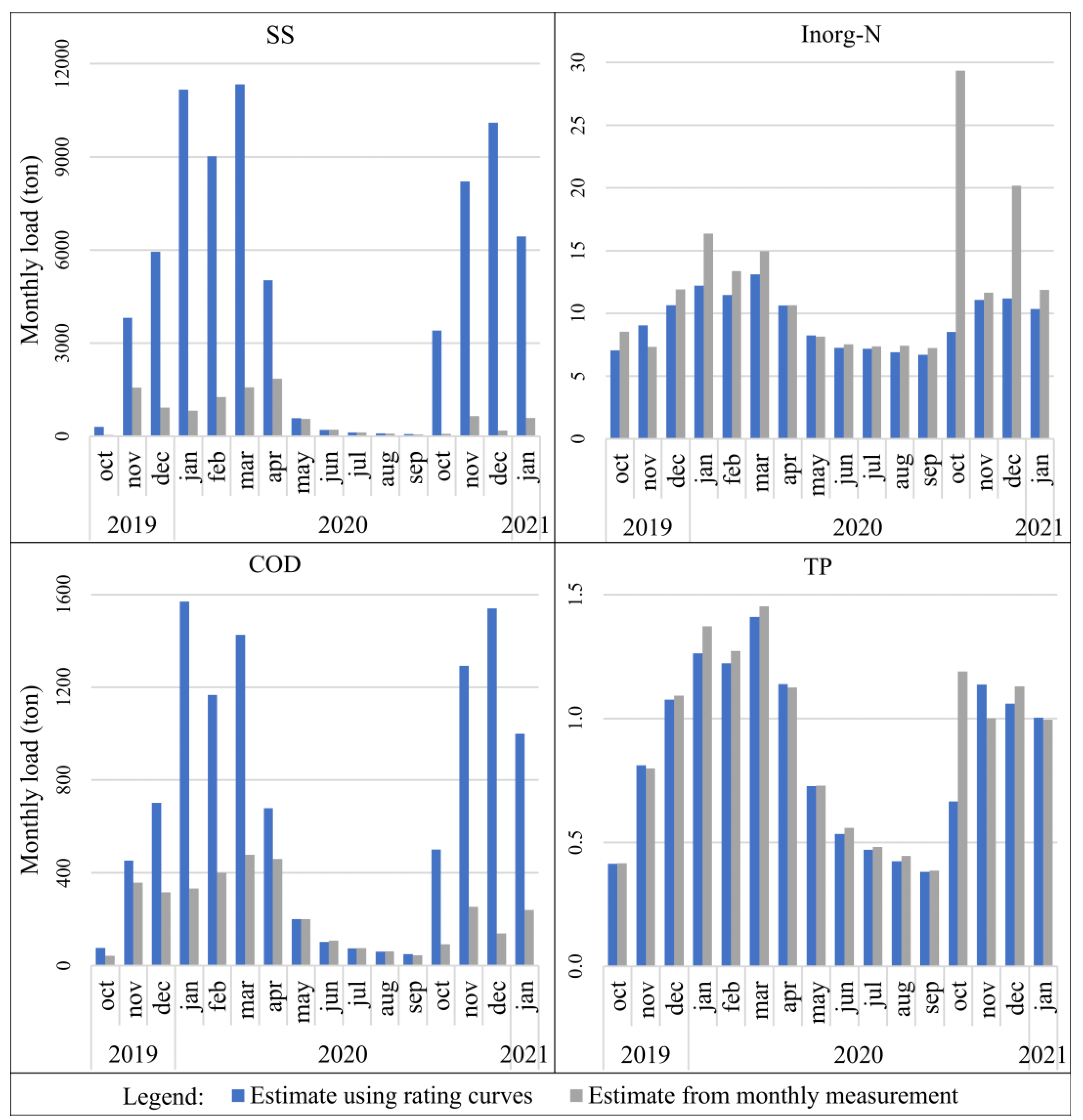
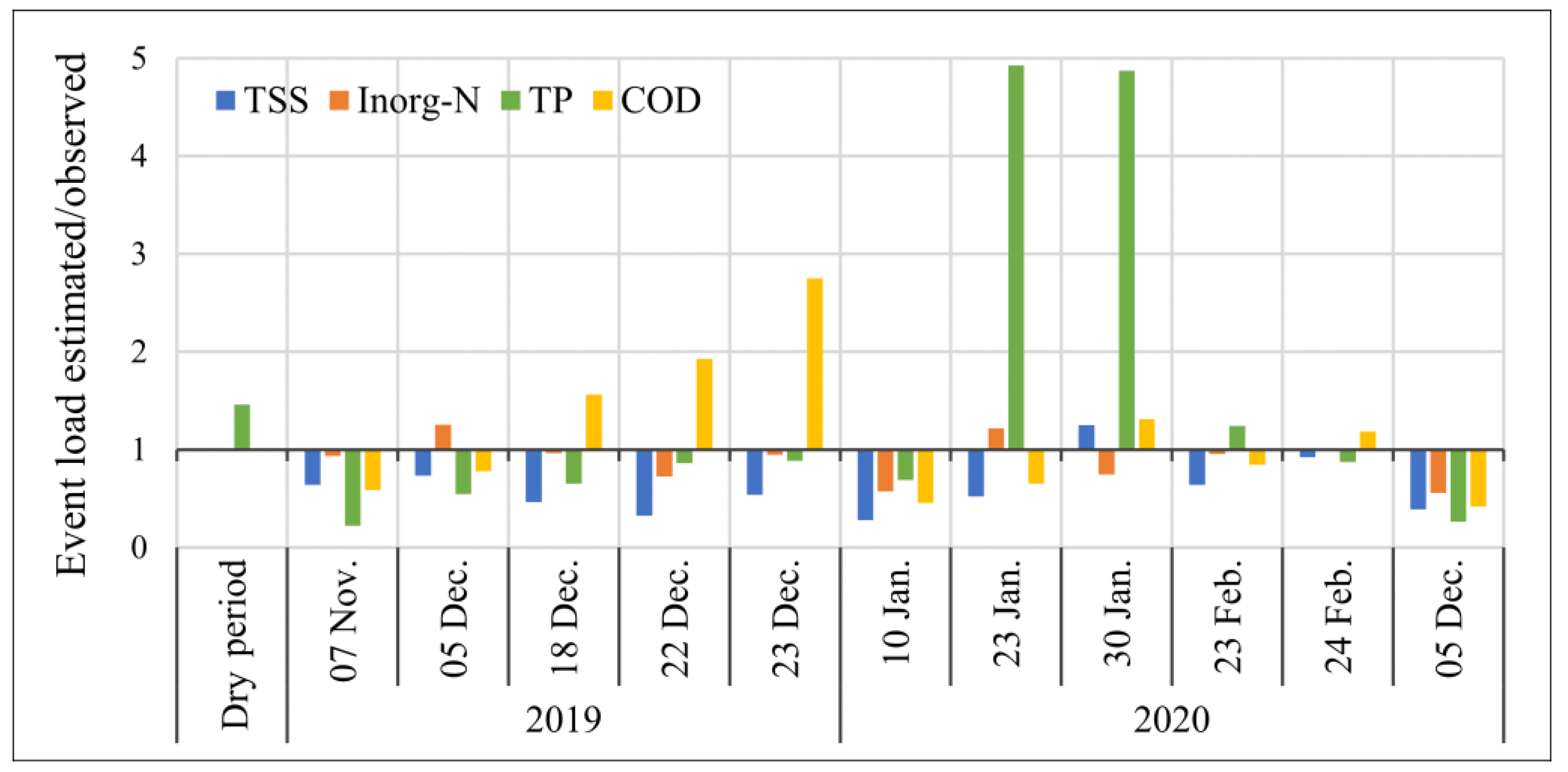
3.4. Estimation of Monthly Pollutant Loads

The accumulated monthly loads estimated by the pollutant rating curves varied widely, especially for the TSS and COD parameters, presenting higher values in rainy months. The TSS loads varied from 70 tons/month to over 11,000 tons/month and the COD loads from approximately 50 tons/month to 1500 tons/month. The rainy season is responsible for almost all the suspended solid pollution and a large part of the COD pollution (Figure 9). Lower values are observed for monthly nutrient loads, and Inorg-N loads are associated with the lowest percentage difference between dry and rainy seasons’ contributions. This happens due to the high nitrogen concentrations found at lower flow rates during the dry period and also between flood events, highlighting the influence of the pollutant loads present all year round. Phosphorus also shows a contribution of the dry season to the annual load, to a lesser extent. The loads ranged from almost 7 to 13 tons/month for Inorg-N and 0.4 to 1.4 tons/month for TP.

In terms of annual unit load for the hydrological year 2019–2020, the resulting estimates are 2239.4 kg TSS/ha.year, 308.0 kg COD/ha.year, 5.2 kg Inorg-N/ha.year, and 0.5 kg TP/ha.year. In a section upstream of the one monitored in this work, Aguiar [69] found annual sediment loads between the years 2011 and 2015 higher than the one in 2019–2020, yet the level of sediment production in the Riacho Fundo basin in this last year can be considered high. This statement is supported by the high TSS loads found by Aquino et al. [59] also for the Riacho Fundo stream and by Costa et al. [20] for the Vicente Pires stream. Barbosa et al. [58] found for the Riacho Fundo basin an estimated annual load of Inorg-N and contribution percentages of each season very similar to the results of this work, and a slightly lower annual TP load and a greater influence of the rainy season on the pollution by this nutrient. The authors also report that the Riacho Fundo stream is the tributary that contributes the most N and P loads to Paranoá Lake.

The unit loads of nitrogen and phosphorus calculated for the whole basin area are lower than those indicated as typical for runoff in residential, commercial, and industrial areas [70], while the unit load of TSS resulted in a value much higher than those of all land uses and more compatible with the load that the author points out as from recently developed urban areas [70]. The unit load of suspended solids was higher than the diffuse pollution load found for a small, urbanized watershed by Brites and Gastaldini [12]; however, it was closer to the higher unit load in a watershed with predominantly rural use, which the authors attribute to soil management and preparation. At the same time, the annual sediment unit load in the Riacho Fundo watershed is much higher than that found by Lopes [63] for a watershed with predominantly rural use also in the Federal District.

The estimation of monthly loads by the monthly monitoring methodology resulted in significantly lower values than those estimated by the rating curves for TSS and COD in the rainy months (underestimation of TSS load in 59 to 98% and COD load in 21 to 91%), while in the dry months the estimates resulted in very close values (differences no larger than 23% for TSS loads and 11% for COD loads). Overall, the monthly monitoring methodology overestimated the monthly loads of Inorg-N and TP compared to the estimation with the curves (up to 34% for Inorg-N loads and 9% for TP loads). Some larger differences between the estimates in the later months of 2020 are linked to data gaps in the continuous flow monitoring.

The graphs provide a better understanding of the difference in the proportions of the estimates (Figure 10), which can be explained by the adoption of only one pollutant concentration value to represent a long period of time and a wide range of flow rates in the monthly monitoring methodology. Therefore, this methodology often extends the pollutant concentration characteristics at low discharges to all discharges, distorting the loading values and not being able to consider the variation in diffuse pollution carried by different flood events as does that of the rating curves.

As a result, the monthly monitoring methodology tends to greatly underestimate suspended solids and COD pollution loads and overestimate nitrogen and phosphorus loads, especially if samples are collected at low flows, since these parameters are strongly correlated with flow rates, increasing substantially in higher discharges. Monthly TSS and COD loads were often of an order of magnitude lower than those found by the rating curve methodology. The monthly monitoring methodology has then no potential to accurately contemplate the diffuse pollution loads of these parameters, and it is better to use the rating curves for their estimation. In this case, it may be advantageous to invest in obtaining a pollutant rating curve with a larger amount of concentration data collected in the field at different flows and events, and installing automatic equipment for continuous level monitoring, such as the one used in this work, to aid water quality monitoring and improve the estimates of pollution loads. This conclusion is consistent with what Park and Engel [70] suggested, that by adding data collected at flood events to the data obtained by uniformly spaced monitoring, there is an improvement in the estimation of annual load in streams.

Conversely, the estimates of nutrient loads by the two methodologies were not so discrepant, mainly because their values are smaller, but these parameters also do not have as strong a connection with increased discharges. Only for nitrogen, the monthly monitoring methodology slightly minimizes the dilution effect of the loads that occurs during the rainy months, though in general it proves to be adequate for estimating the order of magnitude of monthly pollution loads for the nutrients studied, including the contribution of diffuse pollution.

4. Conclusions

Diffuse pollution monitoring in the Riacho Fundo watershed showed strong impacts of flood events on the water quality of the stream, most notably for solids and COD loads. Nutrient loading presented a more continuous behavior, even in the dry season, particularly nitrogen, probably supplied by irregular sewage discharges and the effluent discharge from a wastewater treatment plant.

Correlations were found between the pollutant EMC and the hydrological characteristics of flood events. Positive correlations between TS, TSS, and COD and mean flow rate and between these parameters and the number of antecedent dry days were observed. Rainfall spatial distribution analysis indicated that the concentration of rainfall over urban areas of the watershed induces higher EMCs of solids and nitrate, while the concentration of rainfall in more rural and native vegetation areas is associated with higher EMCs of ammonia and COD.

The pollutant rating curves developed in this work were found to be adequate for estimating accumulated loads. The estimates for the Riacho Fundo watershed indicate high monthly loads of TSS, Inorg-N, TP, and COD. The study indicated that load estimation from water quality data based on monthly monitoring is not adequate for TSS and COD due to the magnitude of loads carried by flood events. In this case, the use of pollutant rating curves coupled with continuous flow monitoring can provide more accurate load estimates. For Inorg-N and TP, the estimates with monthly monitoring and with the rating curves produce compatible results in order of magnitude, showing that the currently adopted monitoring scheme is adequate for estimating nutrient loads.

It is extremely important to determine the pollution loads that reach the Paranoá Lake, mainly through the Riacho Fundo stream, because the impacts of silting and eutrophication are under course. The application of the pollutant rating curves developed in this work could only be evaluated on the events where the data for their development were obtained. Given the limitations faced in collecting field data, it is recommended that the curves be incremented with more measurements at more flood events and during low flow conditions, and the load estimates be evaluated against data from other events for verification purposes. This becomes important as the accurate estimation of pollutant loads is essential to support the management of the lake as well as the water resources in the Riacho Fundo watershed, providing correct and relevant information for planning actions such as proposing mitigation measures to reduce the impacts of diffuse pollution.

References

1. Yazdanfar, Z.; Sharma, A. Urban drainage system planning and design—Challenges with climate change and urbanization: A review. Water Sci. Technol. 2015, 72, 165–179. [Google Scholar] [CrossRef] [PubMed] [Green Version]
2. Sharma, S. Water Challenges of an Urbanizing World. In Management of Cities and Regions; Bobek, V., Ed.; IntechOpen: London, UK, 2017; pp. 99–111. [Google Scholar] [CrossRef] [Green Version]
3. Novotny, V.; Goodrich-Mahoney, J. Comparative assessment of pollution loadings from non-point sources in urban land use. Prog. Water Technol. 1978, 10, 775–785. [Google Scholar]
4. Goonetilleke, A.; Thomas, E.; Ginn, S.; Gilbert, D. Understanding the role of land use in urban stormwater quality management. J. Environ. Manag. 2005, 74, 31–42. [Google Scholar] [CrossRef] [PubMed] [Green Version]
5. Novotny, V. The next step—Incorporating diffuse pollution abatement into watershed management. Water Sci. Technol. 2005, 51, 1–9. [Google Scholar] [CrossRef] [PubMed]
6. Reinelt, L.E.; Horner, R.R.; Castensson, R. Non-point source water pollution management: Improving decision-making information through water quality monitoring. J. Environ. Manag. 1992, 34, 15–30. [Google Scholar] [CrossRef]
7. Ferrier, R.C.; D’Arcy, B.J.; MacDonald, J.; Aitken, M. Diffuse pollution—What is the nature of the problem? Water Environ. J. 2005, 19, 361–366. [Google Scholar] [CrossRef]
8. Meals, D.W.; Richards, R.P.; Dressing, S.A. Pollutant Load Estimation for Water Quality Monitoring Projects; Tech Notes 8, Developed for U.S. Environmental Protection Agency; Tetra Tech, Inc.: Fairfax, VA, USA, 2013. Available online: https://www.epa.gov/polluted-runoff-nonpoint-source-pollution/nonpoint-source-monitoring-technical-notes (accessed on 11 May 2022).
9. Yazdi, M.N.; Sample, D.J.; Scott, D.; Wang, X.; Ketabchy, M. The effects of land use characteristics on urban stormwater quality and watershed pollutant loads. Sci. Total Environ. 2021, 773, 145358. [Google Scholar] [CrossRef]
10. Righetto, A.M.; Gomes, K.M.; Freitas, F.R.S. Poluição difusa nas águas pluviais de uma bacia de drenagem urbana. Eng. Sanit. E Ambient. 2017, 22, 1109–1120. [Google Scholar] [CrossRef] [Green Version]
11. Tsuji, T.M.; Costa, M.E.L.; Koide, S. Diffuse pollution monitoring and modelling of small urban watershed in Brazil Cerrado. Water Sci. Technol. 2019, 79, 1912–1921. [Google Scholar] [CrossRef] [PubMed]
12. Brites, A.P.Z.; Gastaldini, M.d.C.C. Avaliação da Carga Poluente no Sistema de Drenagem de Duas Bacias Hidrográficas Urbanas. Rev. Bras. Recur. Hídricos 2007, 12, 211–221. [Google Scholar]
13. Vieira, P.C.; Seidl, M.; Nascimento, N.O.; Sperling, M.V. Avaliação de Fluxo de poluentes em Tempo seco e Durante Eventos de Chuva em uma Microbacia Urbanizada no Município de belo Horizonte, Minas Gerais. In Manejo de águas pluviais urbanas; Righetto, A.M., Ed.; ABES: Rio de Janeiro, Brazil, 2009; pp. 346–366. [Google Scholar]
14. Chen, L.; Dai, Y.; Zhi, X.; Xie, H.; Shen, Z. Quantifying nonpoint source emissions and their water quality responses in a complex catchment: A case study of a typical urban-rural mixed catchment. J. Hydrol. 2018, 559, 110–121. [Google Scholar] [CrossRef]
15. Kozak, C.; Fernandes, C.V.S.; Braga, S.M.; Prado, L.L.; Froehner, S.; Hilgert, S. Water quality dynamic during rainfall episodes: Integrated approach to assess diffuse pollution using automatic sampling. Environ. Monit. Assess. 2019, 191. [Google Scholar] [CrossRef] [PubMed]
16. Li, J.; Li, H.; Shen, B.; Li, Y. Effect of non-point source pollution on water quality of the Weihe River. Int. J. Sediment. Res. 2011, 26, 50–61. [Google Scholar] [CrossRef]
17. Freire, R.; Bonifácio, C.M.; de Freitas, F.H.; Schneider, R.M.; Tavares, C.R.G. Formas nitrogenadas e fósforo total em cursos d’água: Estudo de caso do ribeirão Maringá, Estado do Paraná. Acta Sci. Technol. 2013, 35, 711–716. [Google Scholar] [CrossRef] [Green Version]
18. Girardi, R.; Pinheiro, A.; Garbossa, L.H.P.; Torres, E. Water quality change of rivers during rainy events in a watershed with different land uses in Southern Brazil. Rev. Bras. Recur. Hídricos 2016, 21, 514–524. [Google Scholar] [CrossRef] [Green Version]
19. Medeiros, W.M.V.; Silva, C.E.; Lins, R.P.M. Avaliação sazonal e espacial da qualidade das águas superficiais da bacia hidrográfica do rio Longá, Piauí, Brasil. Rev. Ambient. Água 2018, 13. [Google Scholar] [CrossRef] [Green Version]
20. Costa, M.E.L.; Koide, S.; Carvalho, D.J.; Garnier, J. Qualidade das águas urbanas no córrego Vicente Pires—Distrito Federal. Rev. Eletrônica De Gestão E Tecnol. Ambient. (GESTA) 2021, 9, 47–68. [Google Scholar] [CrossRef]
21. Donigian, A.S.; Huber, W.C. Modeling of Non Point Sources Water Quality in Urban and Non-Urban Areas; U.S. Environmental Protection Agency Technical Report; USEPA: Washington, DC, USA, 1991. Available online: https://nepis.epa.gov/Exe/ZyPURL.cgi?Dockey=30000OTC.txt%0A (accessed on 11 May 2022).
22. Lin, J.P. Review of Published Export Coefficient and Event Mean Concentration (EMC); Technical Note; Wetlands Regulatory Assistance Program; U.S. Army Engineer Research and Development Center: Vicksburg, MS, USA, 2004. Available online: https://hdl.handle.net/11681/3547 (accessed on 11 May 2022).
23. Richards, R.P. Estimation of Pollutant Loads in Rivers and Streams: A Guidance Document for NPS Programs; U.S. Environmental Protection Agency: Tiffin, OH, USA, 1998. [Google Scholar]
24. Vaze, J.; Chiew, F.H.S. Comparative evaluation of urban storm water quality models. Water Resour. Res. 2003, 39, 1–10. [Google Scholar] [CrossRef]
25. Tsihrintzis, V.A.; Hamid, R. Modeling and management of urban stormwater runoff quality: A review. Water Resour. Manag. 1997, 11, 136–164. [Google Scholar] [CrossRef]
26. Borah, D.K.; Bera, M. Watershed-Scale Hydrologic and Nonpoint-Source Pollution Models: Review of Applications. Trans. ASAE 2013, 47, 789–803. [Google Scholar] [CrossRef] [Green Version]
27. Park, Y.S.; Engel, B.A. Use of Pollutant Load Regression Models with Various Sampling Frequencies for Annual Load Estimation. Water 2014, 6, 1685–1697. [Google Scholar] [CrossRef] [Green Version]
28. Crawford, C.G. Estimation of suspended-sediment rating curves and mean suspended-sediment loads. J. Hydrol. 1991, 129, 331–348. [Google Scholar] [CrossRef]
29. Lapong, E.; Fujihara, M.; Izumi, T.; Kobayashi, N.; Kakihara, T. Suspended Load Estimation in Rivers in Agricultural Areas Using Regression Analyses with Data Stratification. J. Water Environ. Technol. 2012, 10, 387–398. [Google Scholar] [CrossRef] [Green Version]
30. Stenback, G.A.; Crumpton, W.G.; Schilling, K.E.; Helmers, M.J. Rating curve estimation of nutrient loads in Iowa rivers. J. Hydrol. 2011, 396, 158–169. [Google Scholar] [CrossRef]
31. Ide, J.; Chiwa, M.; Higashi, N.; Maruno, R.; Mori, Y.; Otsuki, K.; Mori, Y. Determining storm sampling requirements for improving precision of annual load estimates of nutrients from a small forested watershed. Environ. Monit. Assess. 2012, 184, 4747–4762. [Google Scholar] [CrossRef] [PubMed]
32. Horowitz, A.J. Determining annual suspended sediment and sediment-associated trace element and nutrient fluxes. Sci. Total Environ. 2008, 400, 315–343. [Google Scholar] [CrossRef] [PubMed]
33. Pellerin, B.A.; Bergamaschi, B.A.; Gilliom, R.J.; Crawford, C.G.; Saraceno, J.; Frederick, C.P.; Murphy, J.C. Mississippi River Nitrate Loads from High Frequency Sensor Measurements and Regression-Based Load Estimation Terms of Use. Environ. Sci. Technol 2014, 48, 12612–12619. [Google Scholar] [CrossRef] [Green Version]
34. Pereira, A. Simulação da eutrofização do Lago Paranoá. Revista DAE 1985, 45, 386–389. [Google Scholar]
35. Menezes, P.H.B.J. Avaliação do efeito das ações antrópicas no Processo de Escoamento Superficial e Assoreamento na bacia do Lago Paranoá. Master’s Thesis, University of Brasília, Brasília, Brazil, 2010. [Google Scholar]
36. Franz, C.; Makeschin, F.; Weiß, H.; Lorz, C. Sediments in urban river basins: Identification of sediment sources within the Lago Paranoá catchment, Brasilia DF, Brazil—Using the fingerprint approach. Sci. Total Environ. 2013, 466–467, 513–523. [Google Scholar] [CrossRef] [PubMed]
37. Oliveira, E.S. Qualidade dos Sedimentos e Análise Multi-temporal do Assoreamento do Lago Paranoá—DF. Ph.D. Thesis, University of Brasília, Brasília, Brazil, 2021. [Google Scholar]
38. Nunes, G. Aplicação do Modelo SWAT no Estudo Hidrológico e de Qualidade da água da Bacia do lago Paranoá—DF. Master’s Thesis, University of Brasília, Brasília, Brazil, 2016. [Google Scholar]
39. Nunes, G.; Minoti, R.T.; Koide, S. Mathematical Modeling of Watersheds as a Subsidy for Reservoir Water Balance Determination: The Case of Paranoá Lake, Federal District, Brazil. Hydrology 2020, 7, 85. [Google Scholar] [CrossRef]
40. Paula, A.C.V. Estudo Experimental e Modelagem da Lagoa de Detenção do Guará-DF: Comportamento no Amortecimento de Cheias e na Alteração da Qualidade da água. Master’s Thesis, University of Brasília, Brasília, Brazil, 2019. [Google Scholar]
41. Costa, M.E.L.; Carvalho, D.J.; Koide, S. Assessment of Pollutants from Diffuse Pollution through the Correlation between Rainfall and Runoff Characteristics Using EMC and First Flush Analysis. Water 2021, 13, 2552. [Google Scholar] [CrossRef]
42. Instituto Nacional de Meteorologia (INMET). 2021. Normais Climatológicas. Available online: https://portal.inmet.gov.br/servicos/normais-climatológicas (accessed on 11 May 2022).
43. Ribeiro, J.F.; Walter, B.M.T. Fitofisionomias do bioma cerrado. In Cerrado: Ambiente e flora; Sano, S.N., Almeida, S.P., Eds.; EMBRAPA-CPAC: Planaltina, Brazil, 1998; pp. 89–166. Available online: http://www.alice.cnptia.embrapa.br/handle/doc/554094 (accessed on 11 May 2022).
44. Infraestrutura de Dados Espaciais do Distrito Federal—IDE/DF. 2021. Cobertura do Solo 2019; Geoportal/DF. Available online: https://www.geoportal.seduh.df.gov.br/geoportal/ (accessed on 15 December 2021).
45. Reatto, A.; Martins, E.S.; Farias, M.F.R.; Silva, A.V.; Carvalho, O.A., Jr. Mapa pedológico digital—SIG atualizado do Distrito Federal Escala 1:100.000 e uma síntese do texto explicativo; Documentos/Embrapa Cerrados n. 120; Embrapa Cerrados: Planaltina, Brazil, 2004. [Google Scholar] [CrossRef]
46. de Araújo Pedron, F.; Dalmolin, R.S.D.; Azevedo, A.C.; Kaminski, J. Solos urbanos. Ciência Rural 2004, 34, 1647–1653. [Google Scholar] [CrossRef]
47. Secretaria Nacional de Saneamento (SNS). 2021. Diagnósticos SNIS 2021/2022. Available online: http://www.snis.gov.br/diagnosticos (accessed on 11 May 2022).
48. American Public Health Association (APHA); American Water Works Association (AWWA); Water Environment Federation (WEF). Standard Methods for the Examination of Water and Wastewater, 23rd ed.; Baird, R.B., Eaton, A.D., Rice, E.W., Eds.; APHA: Washington, DC, USA; AWWA: Denver, CO, USA; WEF: Alexandria VA, USA, 2017. [Google Scholar]
49. Lee, J.H.; Bang, K.W.; Ketchum, J.H.; Choe, J.S.; Yu, M.J. First flush analysis of urban storm runoff. Sci. Total Environ. 2002, 293, 163–175. [Google Scholar] [CrossRef]
50. Novotny, V. Unit Pollutant Loads. Water Environ. Technol. 1992, 4, 40–43. Available online: http://www.jstor.org/stable/24661272 (accessed on 11 May 2022).
51. Peng, H.-Q.; Liu, Y.; Wang, H.-W.; Gao, X.-L.; Ma, L.-M. Event mean concentration and first flush effect from different drainage systems and functional areas during storms. Environ. Sci. Pollut. Res. 2016, 23, 5390–5398. [Google Scholar] [CrossRef]
52. Choi, J.; Park, B.; Kim, J.; Lee, S.; Ryu, J.; Kim, K.; Kim, Y. Determination of NPS Pollutant Unit Loads from Different Landuses. Sustainability 2021, 13, 7193. [Google Scholar] [CrossRef]
53. Perera, T.; Mcgree, J.; Egodawatta, P.; Jinadasa, K.B.S.N.; Goonetilleke, A. Catchment based estimation of pollutant event mean concentration (EMC) and implications for first flush assessment. J. Environ. Manag. 2021, 279, 111737. [Google Scholar] [CrossRef]
54. Kozak, C. Water Quality Assessment and its Effects on Diffuse Pollution Considering a New Water Quality and Quantity Approach. Master’s Thesis, Federal University of Paraná, Curitiba, Brazil, 2016. [Google Scholar]
55. Nogueira, F.F. Métodos para monitoramento e estimativa de cargas poluidoras difusas em bacias hidrográficas. Master’s Thesis, University of São Paulo, São Paulo, Brazil, 2020. [Google Scholar]
56. Menezes, D.; Marcuzzo, F.F.N.; Pedrollo, M.C.R. Estimativa da produção de sedimentos utilizando a curva-chave de sedimentos. Ci. e Nat. 2021, 43, 1–31. [Google Scholar] [CrossRef]
57. Governo do Distrito Federal (GDF). Relatório Final—Volume I—Diagnóstico; Plano de Gerenciamento Integrado de Recursos Hídricos do Distrito Federal; GDF: Brasília, Brazil, 2012.
58. Barbosa, J.S.B.; Bellotto, V.R.; Silva, D.B.; Lima, T.B. Nitrogen and Phosphorus Budget for a Deep Tropical Reservoir of the Brazilian Savannah. Water 2019, 11, 1205. [Google Scholar] [CrossRef] [Green Version]
59. Aquino, I.G.; Roig, H.L.; Oliveira, E.S.; Garnier, J.; Guimarães, E.M.; Koide, S. Variação temporal da descarga sólida em suspensão e identificação de minerais a partir de aperfeiçoamento de método de amostragem automática no Córrego Riacho Fundo, Brasília, Distrito Federal. Geol. USP Série Científica 2018, 18, 171–185. [Google Scholar] [CrossRef] [Green Version]
60. De França Lopes, L.L.; De Sousa Diniz, L.A.; Costa, M.E.L.; Koide, S. Análise do comportamento qualitativo de uma lagoa de detenção no Distrito Federal. In Proceedings of the XIII Encontro Nacional de Águas Urbanas, Porto Alegre, Brazil, 19–20 October 2020. [Google Scholar]
61. Távora, B.E. Zona Ripária De Cerrado: Processos Hidrossedimentológicos. Ph.D. Thesis, University of Brasília, Brasília, Brazil, 2017. [Google Scholar]
62. Lopes, G.R. Estudos hidrológicos e hidrossedimentológicos na bacia do córrego do Capão Comprido, DF. Master’s Thesis, University of Brasília, Brasília, Brazil, 2010. [Google Scholar]
63. Fim, B.M. Análises quantitativa e qualitativa das águas superficiais da bacia hidrográfica do ribeirão Rodeador/DF para avaliação das cargas de poluição. Master’s Thesis, University of Brasília, Brasília, Brazil, 2018. [Google Scholar]
64. Quinatto, J.; De Nale Zambelli, N.L.; Souza, D.H.; Neto, S.L.R.; Cardoso, J.T.; Skoronski, E. Using the pollutant load concept to assess water quality in an urban river: The case of Carahá River (Lages, Brazil). Rev. Ambiente Água 2019, 14. [Google Scholar] [CrossRef]
65. Kozak, C.; Fernandes, C.V.S. A influência dos eventos de chuva na contribuição da poluição não pontual para a qualidade da água dos rios. In Proceedings of the XXIV Simpósio Brasileiro de Recursos Hídricos, Belo Horizonte, Brazil, November 2021. [Google Scholar]
66. Park, M.; Choi, Y.S.; Shin, H.J.; Song, I.; Yoon, C.G.; Choi, J.D.; Yu, S.J. A comparison study of runoff characteristics of non-point source pollution from three watersheds in South Korea. Water 2019, 11, 966. [Google Scholar] [CrossRef] [Green Version]
67. Mallin, M.A.; Johnson, V.L.; Ensign, S.H.; Johnson, V.L.; Ensign, S.H. Comparative impacts of stormwater runoff on water quality of an urban, a suburban; a rural stream. Environ. Monit. Assess. 2009, 159, 475–491. [Google Scholar] [CrossRef] [PubMed]
68. Moriasi, D.N.; Gitau, M.W.; Pai, N.; Daggupati, P. Hydrologic and water quality models: Performance measures and evaluation criteria. Trans. ASABE 2015, 58, 1763–1785. [Google Scholar] [CrossRef] [Green Version]
69. Aguiar, M.R.F. Análise da Descarga Sólida em Suspensão na Bacia do Córrego Riacho Fundo, Brasília-DF. Master’s Thesis, University of Brasília, Brasília, Brazil, 2015. [Google Scholar]
70. Marsalek, J. Pollution Due to Urban Runoff: Unit Loads and Abatement Measures; Environmental Hydraulics Section, Hydraulics Research Division, National Water Research Institute, Canada Centre for Inland Waters: Burlington, ON, Canada, 1978. [Google Scholar]
Figure 1. Location of the Riacho Fundo watershed and the rainfall and fluviometric monitoring stations.
Water 14 02354 g001
Figure 2. Land cover map of the Riacho Fundo watershed.
Water 14 02354 g002
Figure 3. Discharge-stage rating curve adjusted to the stream gauging station for the period between October/2019 and July/2020 and its corresponding equations.
Water 14 02354 g003
Figure 4. Boxplot of the concentrations measured in the samples collected at the stream gauging station in the flood events and during the dry period for the parameters of (A) solids (mg/L) and turbidity (NTU); (B) conductivity (μS/cm); (C) COD (mg/L); (D) nitrogen (mg/L); and (E) phosphorus (mg/L).
Water 14 02354 g004
Figure 5. Maps of the spatial distribution of rainfall in the events with water quality monitoring.
Water 14 02354 g005
Figure 6. Pollutant rating curves fitted to the observed data in the Riacho Fundo stream.
Water 14 02354 g006
Figure 7. Ratio between pollutant loading rate estimated by the rating curves and observed.
Water 14 02354 g007
Figure 8. Ratio between total accumulated pollutant load at the event estimated by the rating curves and observed.
Water 14 02354 g008
Figure 9. Contribution of the rainy (October–April) and dry (May–September) seasons to the estimated total annual pollutant load for the hydrological year 2019–2020 in the Riacho Fundo watershed.
Water 14 02354 g009
Figure 10. Monthly loads estimated by the two different methodologies.
Water 14 02354 g010