A Case Study of Tidal Analysis Using Theory-Based Artificial Intelligence Techniques for Disaster Management in Taehwa River, South Korea

Abstract

Monitoring tidal dynamics is imperative to disaster management because it requires a high level of precision to avert possible dangers. Good knowledge of the physical drivers of tides is vital to achieving such a precision. The Taehwa River in Ulsan City, Korea experiences tidal currents in the estuary that drains into the East Sea. The contribution of wind to tide prediction is evaluated by comparing tidal predictions using harmonic analysis and three deep learning models. Harmonic analysis is conducted on hourly water level data from 2010–2021 using the commercial pytides toolbox to generate constituents and predict tidal elevations. Three deep learning models of long short-term memory (LSTM), gated recurrent unit (GRU), and bi-directional lstm (BiLSTM) are fitted to the water level and wind speed to evaluate wind and no-wind scenarios. Results show that Taehwa tides are categorized as semidiurnal tides based on a computed form ratio of 0.2714 in a 24-h tidal cycle. The highest tidal range of 0.60 m is recorded on full moon spring tide indicating the significant lunar pull. Wind effect improved tidal prediction NSE of optimal LSTM model from 0.67 to 0.90. Knowledge of contributing effect of wind will inform flood protection measures to enhance disaster preparedness.

1. Introduction

Tidal rivers experience significant variations in flow, water level and tidal fluctuations contribute significantly to coastal ecosystem services due to the effects of tides [1]. Commonly, these rivers have short reaches with a high overall discharge. A tidal river may be affected by surges, sea-level variations and tides, even though the river may contain low salinity [2]. Astronomic tides are caused by celestial pull which creates gravitational tidal forces from the Sun and the Moon. Tidal forces create significant tidal heights which are greatly affected by water depth, storms, refraction and diffraction, and shoaling [3,4]. To ease computational complexity, the insignificant contribution of gravitational forces from other planetary bodies can be ignored because their effects are several orders of magnitude weaker than those of the Sun and the Moon. Interestingly, the moon exerts more tidal force on near water bodies than the gravitational pull of the sun.

Tidal prediction of sea level hydrodynamics has been conducted globally and several oceanographic computer applications have been developed to study the complex relationship by applying harmonic constants. The common practice in tidal analysis research is to fit machine learning models to observed tidal elevations and meteorological forcings but our study hybridized the classical harmonic analysis with deep learning models with the use of hourly water level data and wind speed only. Additionally, the focus has only been limited to seas and coastal waters for ship navigation planning [5,6] and ocean current assessment [2]. However, estuaries also experience tidal effects due to mean sea level rise. The south coast of South Korea is extremely vulnerable to coastal disasters. Water disasters such as storm surges, hurricanes, typhoons, high tides, and fluvial flooding which cause huge storm damage are greatly affected by extreme wind speed because strong winds with low atmospheric pressure increase water level build-up above normal elevations [7,8,9,10,11,12]. The Taehwa River experiences similar tidal fluctuations at its estuary which drains into the East Sea in Korea thereby generating erratic water levels and modelling uncertainties [13]. This has created the need to assess tidal fluctuations within the watershed through conventional and artificial intelligence methods to mitigate disaster risks, inform water-borne navigation, and coastal water quality assessment, and analyse the contribution of wind to the prediction of tides using a theory-guided harmonic analysis approach which considers constituents estimated from the location of celestial bodies and the deep learning black box models [13,14]. Based on the literature, there has not been a reported study on the combination of harmonically-generated tides with deep learning techniques to analyse lunar and wind effects on tide occurrence. We theorized that with abundant and reliable hourly water level data, harmonic analysis and deep learning modelling can be conducted to understand the wind effect (excluding other meteorological parameters) on the prediction of tides. This showcases the novelty of this research.

A recent study investigated the integration of tidal effect in modeling and mapping of the flood occurrence in Kota Tinggi Johor Malaysia, to reveal that tidal effect with Light Detection and Ranging data (LIDAR) and Hydrologic Engineering Center’s River Analysis System (HEC-RAS) software simulated peak flow hydrograph during the flood event having results of 625.3 m³/s and 743.9 m³/s for December and January floods respectively [15]. However, when the tidal effect was ignored, the simulated flood depth was 43% lower than the observed flow [15]. Recurrent flood events in Malaysia are mainly caused by torrential rainfall, rapid land use changes, poor drainage systems, and tides [16,17]. This underscores the importance of tidal analysis in water resources planning and management. Research on the effects of dam construction on tidal reach has also gained prominence in recent times [18,19,20].

Further research advances in the field of artificial intelligence for tide prediction were reported by [21,22,23,24]. The Long Short Term Memory (LSTM) model performed optimally for 1 h ahead prediction of water level during a storm surge in the Yangtze River Estuary in the East Sea and could make a 15 h ahead prediction with limited error [21]. In another study [22], tested the predictive ability of the Non-linear Autoregressive Exogenous (NARX), neural network models, while considering meteorological data, astronomical tides, and lagged value of observed sea level data to forecast extreme values of high tides in the Venice Lagoon. Results showed that the two models which considered meteorological inputs and without exhibited higher predictive accuracy across all lag times compared to statistical and deterministic models used at the tidal station. Also, the multivariate adaptive regression splines (MARS) outperformed the backpropagation artificial neural network model (BPANN) in estimating solid earth tides in five regions of Ghana [25]. Numerical and artificial models failed to predict peak wave heights at two ports in the Persian Gulf using ANN, extreme learning machine, and support vector regression models and there is a need to explore other modelling approaches to achieve better performance [26].

Time series analysis has also been applied to non-linear streamflow prediction based on Self-Exciting Threshold Autoregressive method (SETAR) and Autoregressive Conditional Heteroscedasticity (ARCH) methods combined with Gene Expression Programming (GEP) for four different rives in East Azerbaijan in Iran [2]. The research showed that the hybrid SETAR-GEP model performed more optimally than the hybrid ARCH-GEP models for the prediction of the monthly streamflow of four rivers. Also, findings proposed several data-preprocessing tasks such as variational mode decomposition (VMD), complete ensemble empirical mode decomposition (CEEMD), and improved CEEMD as data decomposition methods to improve streamflow prediction [27]. Another study revealed that internal pressure is a critical factor for forecasting the discharge coefficient of inflatable dams [28]. When internal pressure was disregarded, prediction accuracy (R²) was reduced by 2.12%. The hybrid Particle Swarm Optimization and Genetic Algorithm (PSO-GA) performed best among other hybrid machine learning models [28]. Another study conducted a literature review of publications focused on the application of artificial intelligence models to river sedimentation and concluded that the main limitations of AI models are their low applicability to other watersheds which have dissimilar morphological and climatic characteristics, and their lack of physical interpretation [29].

In this research, we conducted a harmonic analysis of hourly water level data obtained at the Taehwa watershed by generating constituents used to create tides, analysed tidal reaction to lunar gravitational pull based on moon phase, and evaluated the effect of wind contribution to tidal prediction with the use of deep learning models instead of machine learning models reported in previous works of [23,24]. Deep learning models perform relatively better than machine learning algorithms especially when abundant training data is available, high computational resources, and in tidal current velocity prediction tasks [24]. Recurrent Neural Network (RNN) models such as Long Short Term Memory (LSTM), Bidirectional LSTM (BiLSTM), and Gated Recurrent Unit (GRU) study temporal dependencies in water data to study patterns, learn and create new features using neurons and cell states as opposed to machine learning algorithms which learn in smaller steps and output numerical values in a form of score or classification. A common limitation of LSTM, BiLSTM, and GRU is the data-hungry tendencies and longer training time. Since there are abundant computer resources and data for this study, these limitations are disregarded.

The objectives of this study are to:

i.

analyse tidal effects of Taehwa River using theory-based deep learning modeling; and

ii.

evaluate contributing effect of wind on tide prediction for disaster prevention and management.

The rest of the study is organised as follows: Section 2 highlights materials and methods like the study area, data collection and model input, harmonic analysis of water level data, methods for the wind effect on tidal prediction using deep learning methods, methods for selection of deep learning models, model selection and autocorrelation analysis to determine input sequence. Section 3 presents results and discussion of harmonic analysis, tidal range based on moon phases, and effect of wind speed on tide prediction while a summary of results and inferences are presented afterwards. Section 4 explains the conclusion with references.

2. Materials and Methods

2.1. Study Area

The Taehwa River, otherwise known as the “Taehwagang” flows across Ulsan City from the West to East in South Korea and has its source from Tapgolsaem Spring on the Baegunsan Mountain. Taehwa River’s drainage area of about 645 km² extends to the neighboring city of Gyeongju and has a river length of 46 km, which mainly lies in the city of Ulsan. Being an enviable source of joy for the native people of Ulsan city, the river has enjoyed so much attention, but the emergence of tidal waves and currents keeps increasing the high flood vulnerability at estuary, leaving behind a huge deposit of sediments, high flood risk and an unpredictable wash-off due to the rise of sea currents. This creates a resonating effect on estuaries and rivers that empty into the East Sea [13]. The water level data is greatly influenced by periodic tidal fluctuations due to seawater intrusion and sediment deposition in the Taehwa River. Figure 1 illustrates the study area.

2.2. Data Collection and Model Input

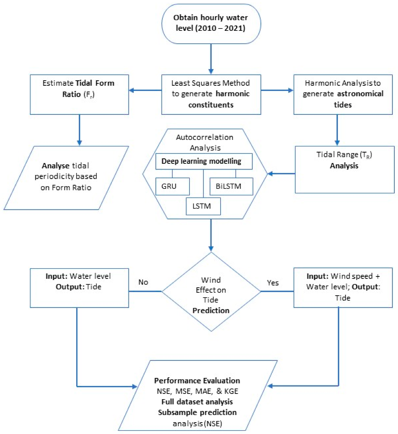
A long-term hourly water level data within the period of 2010–2021 was obtained from Taehwa river automatic gage station located at latitude 35°33′10″ N and longitude 129°1′33″ E and was preprocessed in python to identify missing data and seasonal water variations of the Taehwa River. Periodic decomposition of raw water level data was conducted using harmonic analysis by extrapolating tidal behavior and isolating residual wave components, then, evaluating the effect of wind on tidal prediction with the use of deep learning models. The two scenarios for the effect of wind and no wind on tidal prediction are presented in the workflow chart in Figure 2.

2.3. Harmonic Analysis of Water Level Data of Taehwa River

On rivers that experience tidal effects like the Taehwa estuary, frequencies and periods of constituents can be easily obtained from available water level data, especially when there is abundant water level data. However, it is quite hard to obtain amplitudes and phases that define the oscillatory and periodic curves of the tides. According to [30], tidal forecasting of sea water level is initiated at first by estimating harmonic constants. Therefore, tidal harmonic analysis of observed water level data was carried out by representing spectral signals and functions obtained from raw water level data and super-imposing such waves through the SciPy’s Least Squares Method in the pytides API python module (https://github.com/sam-cox/pytides; accessed on 3 February 2022) to estimate amplitudes and constituents. The Least Squares method proposes a set of solutions that tries to minimize the squared sum of differences between the actual and fitted values [31], as indicated in Equation (1).

$$∆={\displaystyle \sum }_{i=1}^n{\left[h_t-h_i\right]}^2$$

(1)

where: $∆$ = Least minimization operator; n = number of values; h_t = actual tidal level; and h_i = fitted tidal level.

The amplitudes and constituents were further processed and used in predicting the periodic tidal of the Taehwa estuary. This was conducted by substituting the estimated constituents and amplitudes into Equation (2) which defines the general expression for the determination of tidal level as presented by [32]. By so doing, we extracted amplitudes (H_i) and phase lags of the greatest possible number of harmonic constituents. This old method forms the basis of a theory-based approach to tidal analysis.

$$h_t=S_o+{\displaystyle \sum }_{i=1}^i{f}_i{H}_i\cos \left[{\sigma }_{i}t+{\left(V_o+u\right)}_i-g_i\right]+r$$

(2)

where:

h_t = tidal level at time t; S_o = mean sea level height obtained from korean datum; i = number of astronomical categories; f_i = node factor; H_i = amplitude of tidal constituent i; σ_i = angular velocity of tidal constituent i; V_o = initial phase of constituent; u = correction angle; g_i =tidal constituent epoch, r = non-astronomical constant for other disaster factors.

We computed the harmonic tidal Form Ratio (F_r) from the calculated amplitudes of the constituents of M2, S2, K1 and O1, as shown in Equation (3) as proposed by [32].

$$F_r=\left(K1+O1\right)/\left(M2+S2\right)$$

(3)

2.4. Effect of Wind on Tidal Prediction Using Deep Learning Models

Aside the celestial gravitational pull that creates tidal responses, local weather patterns and wind may also affect tides. In addition, weather-induced effects on tides may create ranges in excess of predicted values resulting to localized flooding. It is reasonable to hypothesize that strong offshore winds may move water away from coastlines while onshore winds may excite water into shorelines to reduce low-tide exposures while causing high waters to be higher than predicted. Also, this wind effect is greatly affected by the topography of the shoreline of Taehwa estuary. A limitation of the tidal harmonic analysis is that wind factor may be hard to integrate into Equation (2). Therefore, we considered a theory-based coupling of harmonic analysis and Artificial Intelligence methods such that the wind effect could be evaluated.

Wind speed data were obtained from the meteorological station located at latitude 35°34′56″ N and longitude 129°20′5″ E within the Taehwa watershed, while three deep learning models were fitted to the tide results and evaluated by the Kling Gupta Efficiency (KGE), Nash Sutcliffe Efficiency (NSE), Mean Squared Error (MSE) and Mean Absolute Error (MAE) indices. To achieve this, we considered two scenarios:

i.

concatenating wind input with water level to predict harmonically generated tides;

ii.

input values of water level without wind data to predict tides.

2.5. Deep Learning Model Selection

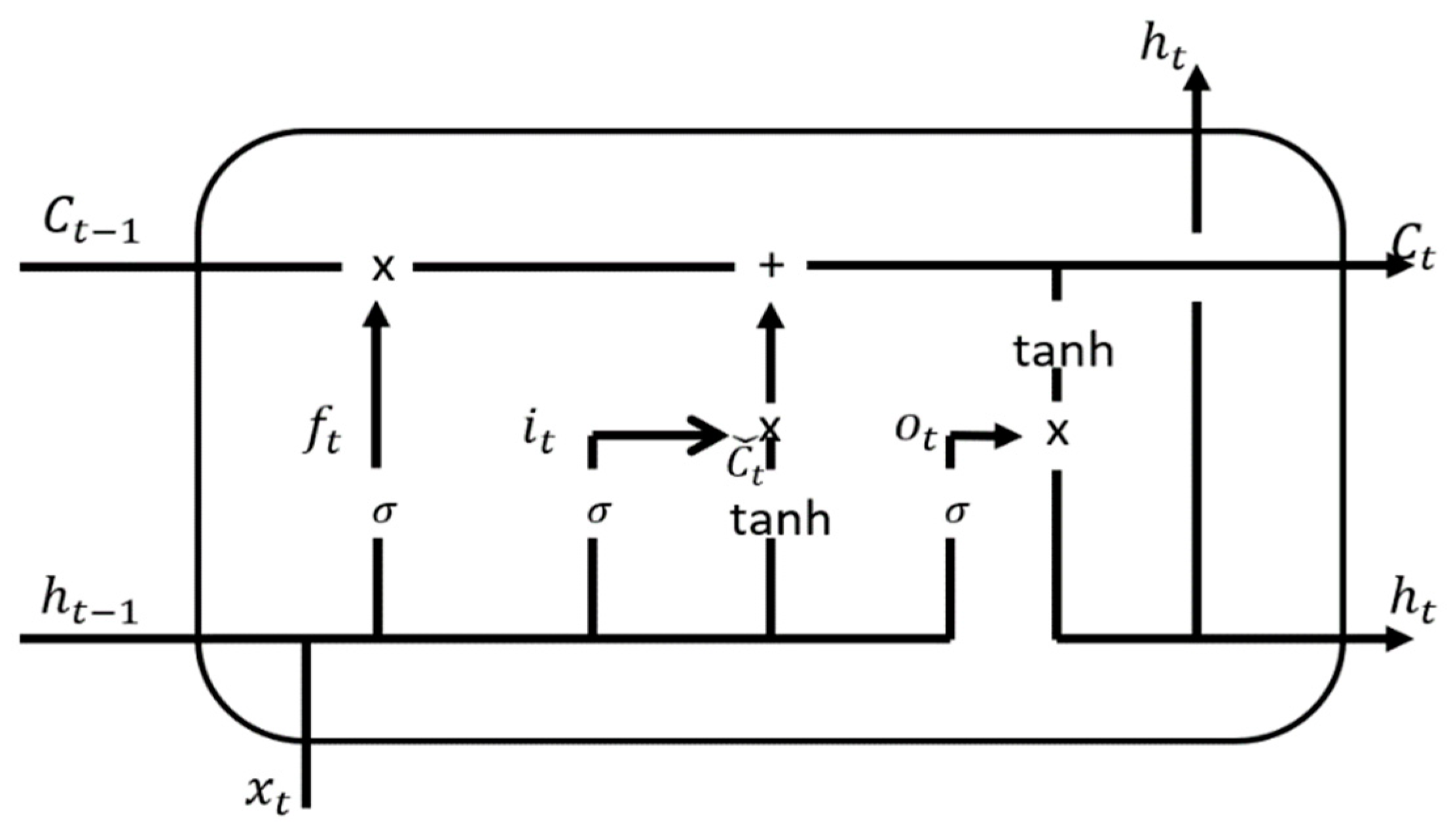
The three models selected for the study are the Long Short Term Memory (LSTM), Bidirectional Long Short Term Memory (Bi-LSTM) and Gated Recurrent Unit (GRU). The LSTM is an example of RNN which learns long temporal dependencies from simple and complex time series data with the use of cell states and gates [33]. The internal architecture of an LSTM model is designed such that there are input gate (i_t), cell states (C_t), output gate (o_t), and forget gate (f_t), which perform functions of water level data input, memory storage, result output, and data filtering respectively. Figure 3 shows the illustration of a simple LSTM model. The LSTM governing equations are presented in Equations (4)–(8).

An improved form of the LSTM model is the BiLSTM model which allows data to be fed into the LSTM model from two directions. At first, water level and wind speed data were passed in the forward direction within the internal structure of the model. Then, information was passed in the backward direction as illustrated in Figure 4. By so doing, the amount of information available for processing and predictive tasks was increased to improve performance.

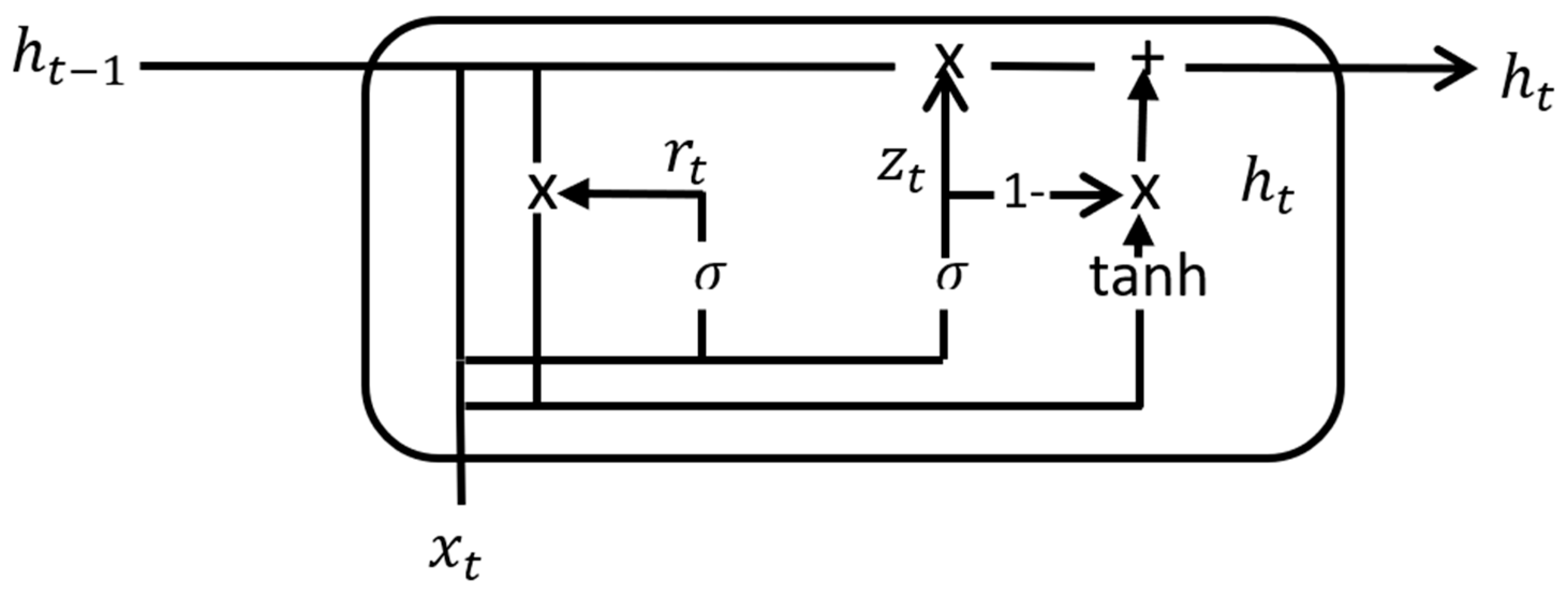
A simpler form of RNN which uses a gating mechanism with two gates namely reset gate and update gate is defined as the GRU model [34] and it is depicted in Figure 5. The gates provide more options for letting information pass through the model.

$$f_t=\sigma \left(W_f·\left[h_{t-1}, x_t\right]+b_f\right)$$

(4)

$$i_t=\sigma \left(W_f·\left[h_{t-1}, x_t\right]+b_i\right)$$

(5)

$$\check{C_t}=\tanh \left(W_c·\left[h_{t-1}, x_t\right]+b_C\right)$$

(6)

$$C_t=f_t\ast C_{t-1}+i_t\ast \check{C_t}$$

(7)

$$o_t=\sigma \left(W_o·\left[h_{t-1}, x_t\right]+b_o\right)$$

(8)

where W, b, h, + or x are weights, biases, states, and pointwise operations respectively.

2.6. Deep Learning Model Creation

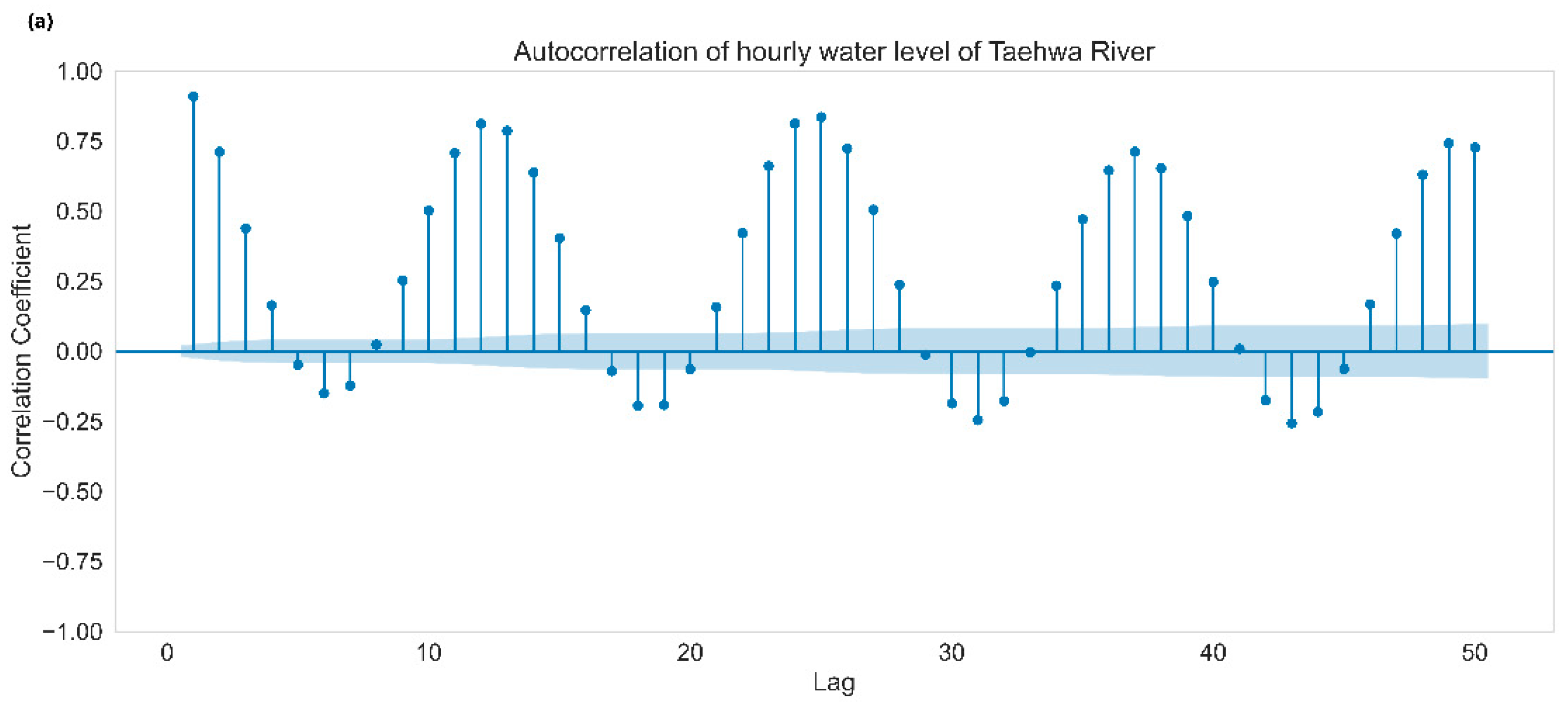
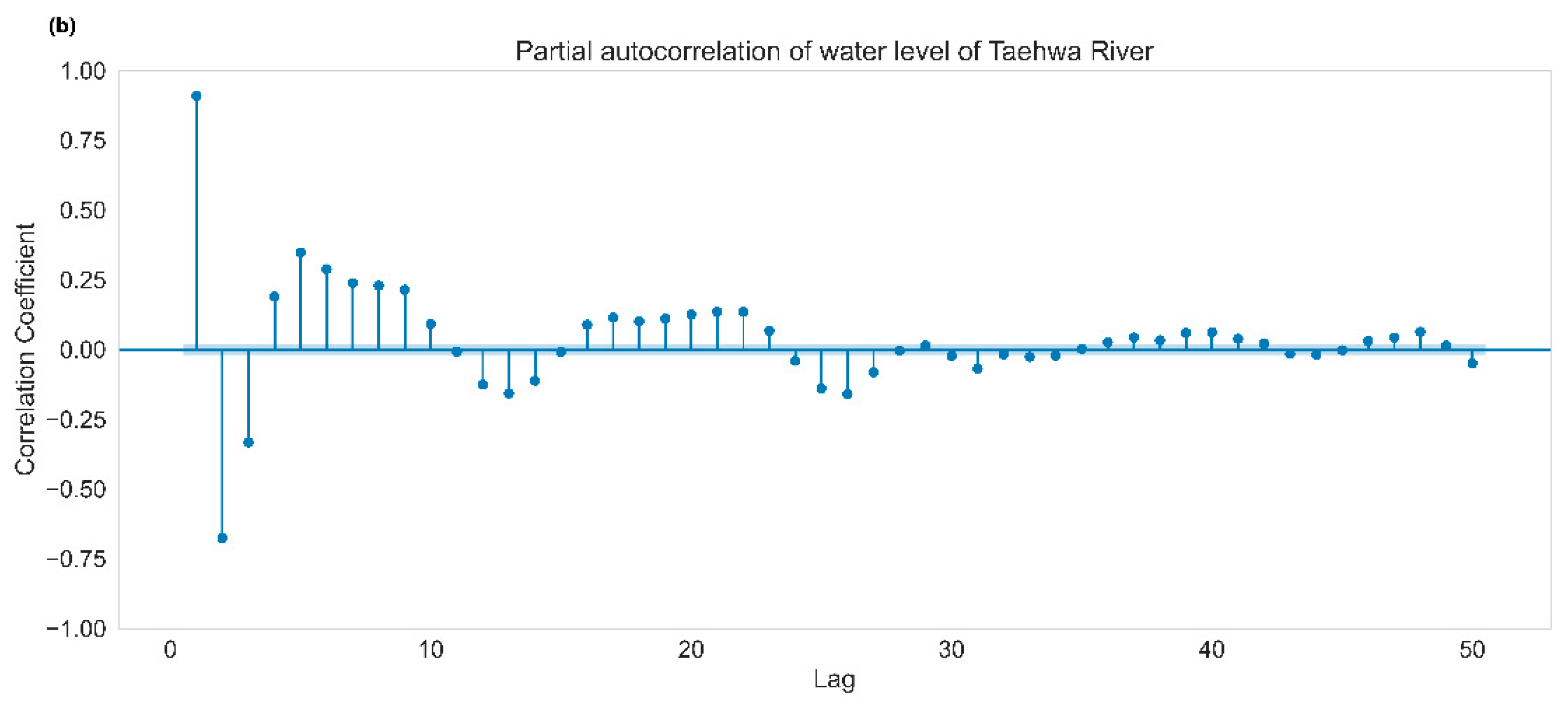
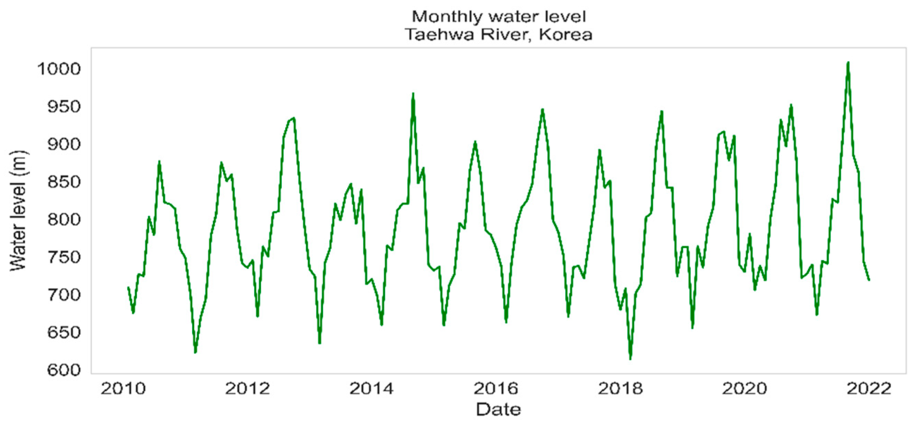
After model selection, we conducted autocorrelation analysis to estimate the optimal input sequence size of water level data and wind speed data that must be used in the modelling task. The autocorrelation function (ACF) and partial autocorrelation function (PACF) use a regressive technique that evaluates a current water level dataset against its lag within a specified confidence interval. A python module—statsmodels—was used for the autocorrelation analysis of the water level data against 50 lag values of itself within a confidence interval of 95%. Figure 6a,b shows the ACF and PACF respectively. It can be observed that there is a trend in the hourly water level towards the 50th data value and almost all lags fall within the 95% confidence interval (the grey shaded area), indicating that all past 50 lags influence the current water level data and are significantly correlated. Therefore a 24-h water level (1 day) was selected as the input sequence. The monthly water level presented in Figure 7 shows that the cumulative monthly water elevation of 1010 m was highest in 2021, mainly due to heavy precipitation and climate change effect in the watershed.

Through a trial-and-error approach, we parameterized the models such that the three models used the same set of hyperparameters to provide a level ground for the comparison of results. Factors considered for hyperparameter selection were model simplicity and lesser computational cost. The final model architecture of 1 neural layer, 64 neurons, ReLu activation function, 0.2% Dropout, Adam optimizer, 128 batch size, and 100 epochs was used to train the GRU, LSTM, and BiLSTM models. Water level data and wind data were divided into 80% train and 20% test sets and fed into the three models. Modelling was conducted on a computer with specifications of Intel (R) Core^TM i7, dual core 3.80 GHz, 3.79 GHZ processor, and 64 GB RAM using python, with Tensorflow [35] and Keras [36] as backend machine learning frameworks. The resulting final model architecture of 1 neural layer, 64 neurons, ReLu activation function, 0.2% Dropout, Adam optimizer, 128 batch size, and 100 epochs was used to train the three models of GRU, LSTM, and BiLSTM.

3. Results and Discussion

3.1. Results of Harmonic Analysis of the Taehwa River

Thirty-eight (38) harmonic constituents were abstracted from the water level through the Least Squares Method as expressed by Equation (2). The harmonic constituents are presented in Supplementary Materials. Tidal Form Ratio (F_r) computed from Equation (3) yielded a value of 0.2714 and was validated using the pytides.tide.form_number command in the pytides module, which yielded the same result. Based on the tidal form classification of [32], we classified the Taehwa river with F_r = 0.2714 as a semidiurnal tide which records two high tides and two low tides in a 24 h tidal period.

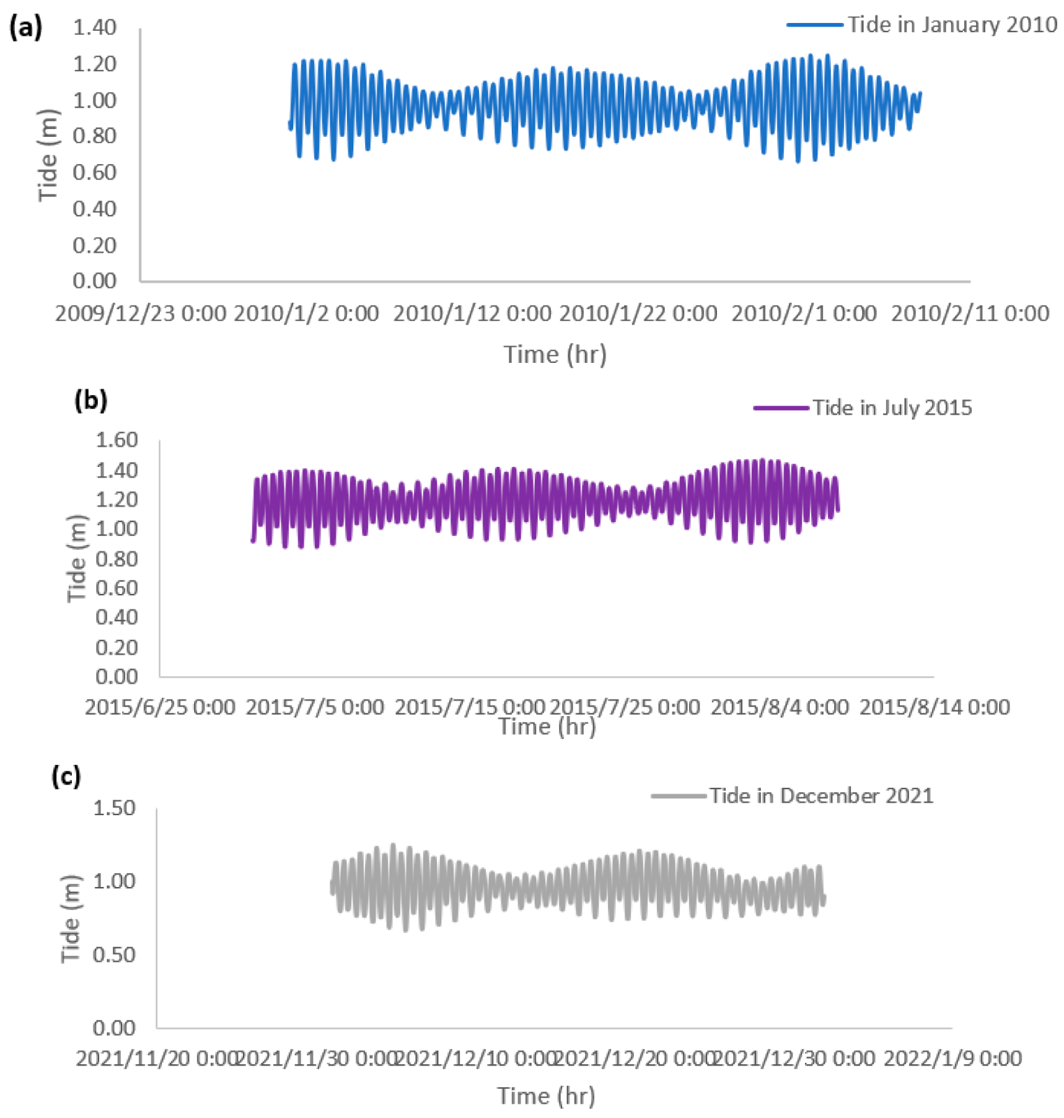
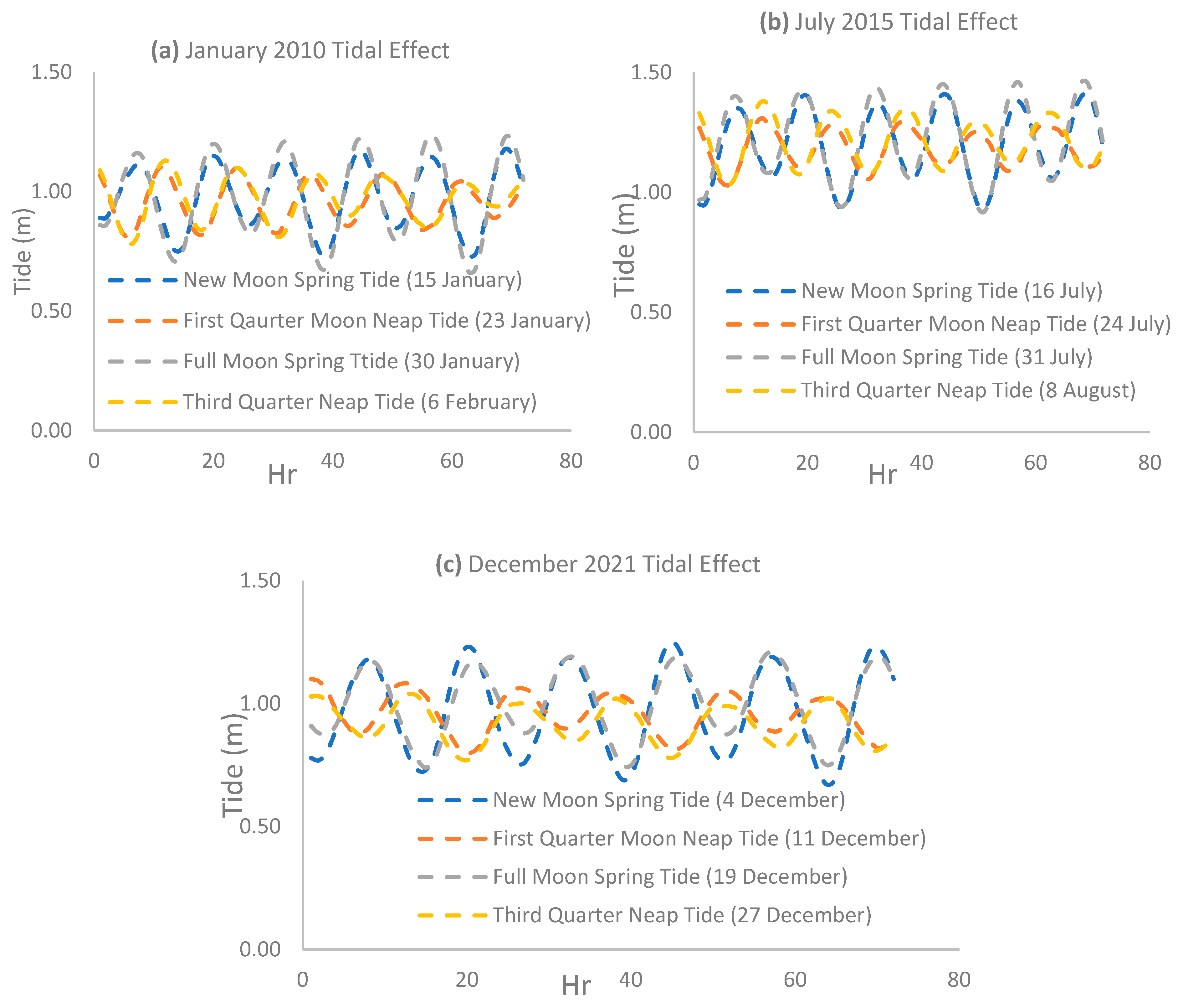
Since tidal analysis is an event-based experiment, at first, we tested the periodicity by visualizing tidal effect results in the Taehwa estuary for January 2010, July 2015, and December 2021, which are representative of the first, middle, and end parts of the long hourly timeseries water level data and are presented in Figure 8a–c. It can be deduced from Figure 8a–c that the Taehwa tides have a periodic and harmonic distribution, as supported by [25]. Monthly tidal oscillations decline steadily towards the first one-third of every month (around the 12th) and rise significantly for the next 10 days, splitting the distribution into three distinct tidal fluctuations per month. The third phase records the highest tidal height and range in the first two cases except in December 2021 because although the East Sea has quite warm waters which intrude into the Taehwa estuary, evaporation is noticeable during this time, thereby, reducing streamflow accumulation and tides.

3.2. Results of Tidal Range across Different Lunar Orientations

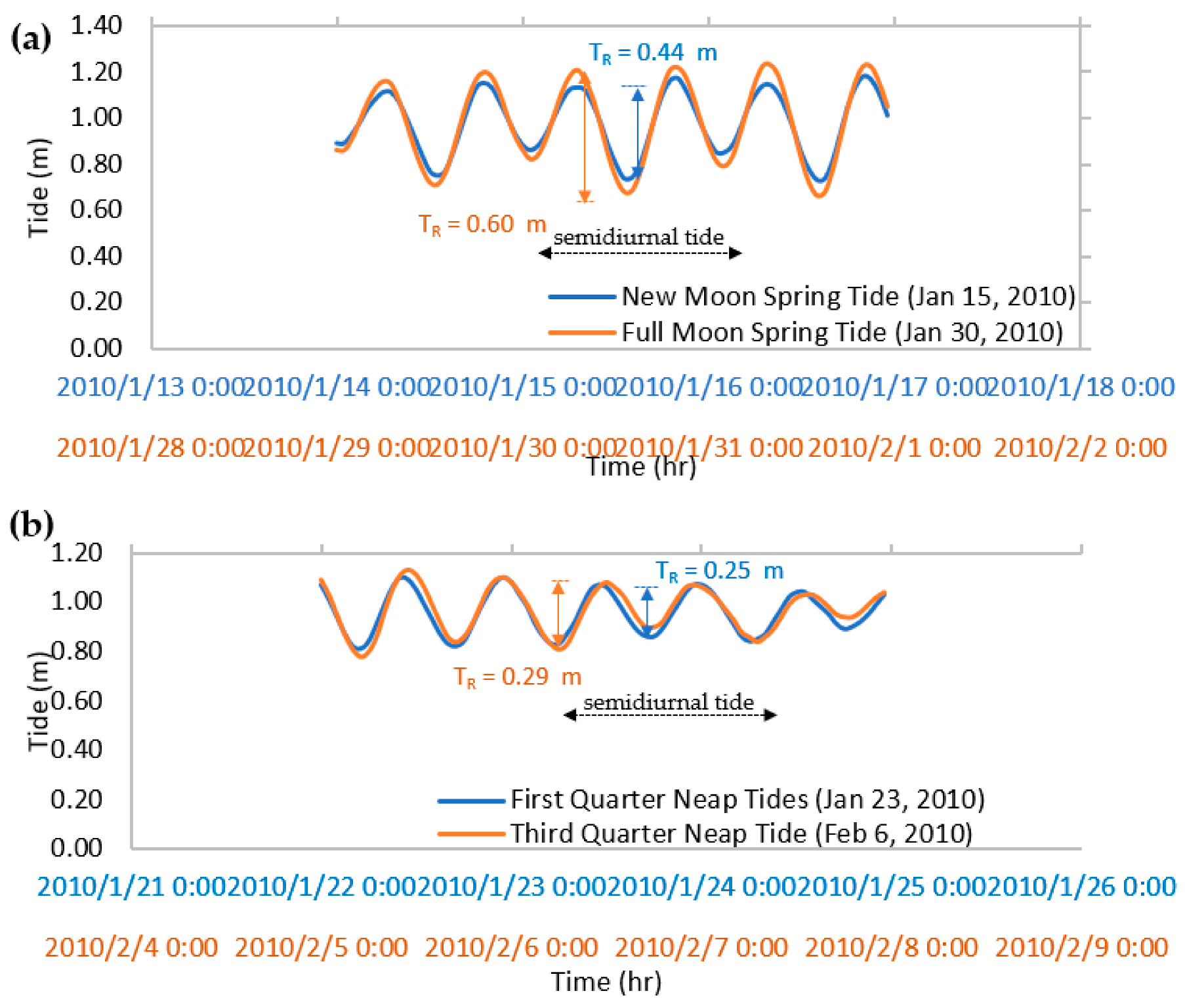
Computation of the tidal range, T_R was carried out for the four lunar phases. Diurnal elevations between adjacent high tides showed no significant difference. This is an indication that the tidal effects of the Taehwa River are purely semidiurnal.

Further analysis of tides on higher temporal scale (daily) and based on four lunar positions of New Moon (NM), First Quarter (FQ), Full Moon (FM), and Third Quarter (TQ) shows high tidal pull exerted by the moon on a full moon and new moon days. High floods are recorded during high tides while there are ebbs during low tides, indicating a need to implement flood protection approaches along the floodplain of the Taehwa River. An example of tidal range computation based on lunar positions for January 2010 is presented in Figure 9a,b.

Moreover, analysis of

Table 1. Tidal range based on moon orientation.

Month	Date	Tide Type	Moon Orientation	Average Tidal Range, TR (m)	Decision
January	15/2010	Spring	NM	0.44
	23/2010	Neap	FQ	0.25	LTL
	30/2010	Spring	FM	0.60	HTL
	6 February 2010	Neap	TQ	0.29
July	16/2015	Spring	NM	0.50
	24/2015	Neap	FQ	0.20	LTL
	31/2015	Spring	FM	0.53	HTL
	7 August 2010	Neap	TQ	0.23
December	4/2021	Spring	NM	0.50	HTL
	11/2021	Neap	FQ	0.27	LTL
	19/2021	Spring	FM	0.43
	27/2021	Neap	TQ	0.34

Note: LTL: lowest tidal level; HTL: Highest tidal level.

shows that the highest tidal level (HTL) was recorded during full moon spring tides with about 67% percentage occurrence (two out of three samples) and a maximum tidal range of 0.60 m. All HTL events occurred during Spring tides with a 100% occurrence, while the lowest tidal level (LTL) receded during the First Quarter of the moon, a point where celestial bodies’ gravitational force vectors act in quadrature with the Earth’s orbits.

To provide a better understanding of the tidal fluctuations based on the size and position of the moon, a superposition of neap and spring tidal waves for all four lunar positions is presented in Figure 10 for the three cases. It can be clearly seen that high tide is recurrent on full moon events of selected years indicating a need to observe caution by Taehwa River users and in extreme events, flood mitigation plans must be implemented. First- and third-quarter neap tides appeared to be less threatening and similar to each other. Tidal peaks appear uniform for full moon and new moon spring tide events while third-quarter moon tides appear slightly higher than first quarter moon tides for the first two cases. With the globally increasing sea level induced by climate change, flooding, drowning, and extreme events may occur during such high tide events. Low tides within the Taehwa estuary might also increase surfing hazards and risks due to lower water levels which reveals rocks and boulders in the river.

3.3. Effect of Wind Speed on Tide Prediction Using Deep Learning Models

Table 2. Test dataset performance evaluation.

Metrics	GRU		LSTM		BiLSTM
	Prediction with No Wind	Prediction with Wind	Prediction with No Wind	Prediction with Wind	Prediction with No Wind	Prediction with Wind
KGE	0.84	0.80	0.82	0.87 *	0.81	0.67
NSE	0.75	0.76	0.83	0.83	0.76	0.67
MSE	0.0059	0.0057	0.0041	0.0041	0.0055	0.0077
MAE	0.06	0.06	0.0502	0.0502	0.0598	0.073

Note: * optimal model across all treatments.

presents the performance indices obtained from the prediction of tidal elevation on the full test dataset with and without wind input for the three models of GRU, LSTM, and BiLSTM. Based on the results of the performance indices, it can be deduced that KGE, SE, NSE, and MAE results of “No wind” input recorded better prediction performance than when the wind data was incorporated into the models. Further exploration of the dataset was performed to ascertain if the insignificant effect of the wind is constant across all datasets and subsample predictions by evaluating NSE values on a subset of prediction data for 7-day, 14-day, 21-day, 28-day, and 35-day predictions, as depicted in Figure 11. Tidal plots are presented in Table S2 of the Supplementary Material. Interestingly, it was discovered that as the number of subsample prediction days increases, the contribution of wind to the prediction of tide increases, especially for the LSTM models which had optimal performance (NSE values written in red). The GRU models competed favorably between the two treatments. However, the BiLSTM failed to capture temporal dependencies in the water level data and wind data, as the case might be.

In summary, tidal fluctuations in the form of flood waves and ebbs which are a source of worry to disaster managers, engineers, and oceanographers are recorded in the Taehwa estuary. Application of the Least Squares method to long hourly water level data (2010–2021) of Taehwa River in Ulsan was conducted to obtain thirty-eight (38) harmonic constituents that fit a set of cosine waves for tidal prediction. According to the classification of [30], the computed tidal form ratio of 0.2714 for the Taehwa River was validated and used to categorize the Taehwa tides as semidiurnal tides having two high tides and two low tides in a 24-h tidal cycle. This finding is supported by the studies [37,38] that the semidiurnal pattern is typical in the East Coast. The generated tides exhibit uniform periodicity typical of semidiurnal tides and this was supported by the findings of [7,8], which confirmed that the tides are periodic waves generated by the pull of the Sun and the Moon. The periodicity of tides makes it easy to explore fluctuations in tidal range and facilitates fitting of cosine curves for modelling tasks. This implies that the wave dynamics within a period of 24 h of the study area can be easily modelled to create policies about the Taehwa river’s water use.

To facilitate the analysis of the large timeseries data, we selected some months as study cases of tidal events based on tidal reports from the Ulsan station. Analysis of monthly and daily tidal range values based on the position and size of the Moon showed that the highest tidal level (HTL) was recorded during the Full Moon with a maximum spring tide of 0.60 m, while the recession of tides was manifest during the First Quarter of the Moon when the Moon and the Sun are at right-angle to the orbits of the Earth. Superimposed neap tides and spring tides during four lunar phases offered more insights into the tidal analysis. First Quarter neap tides and Third Quarter neap tides show an almost similar trend and value. This result agrees with the work of [1,11,39] that neap tides record lesser gravitational pull by celestial bodies. Practically, the results of lunar phases as they affect tide dynamics indicate clearly that high tides are most prevalent during a full moon. River users must enhance disaster preparedness and risk management so that preventive measures for flooding can be implemented during days of high tides which have been identified by the position of the moon. Storm surges, high waves, and other coastal hazards can be easily averted when moon phases and wind speed can be predicted or provided early.

The performance of deep learning models was assessed to evaluate the contribution of wind to the prediction of tides using LSTM, GRU, and BiLSTM. At first, the models were set up to predict tides on the full test dataset after data splitting. Then, the three models were used to predict daily subsets of data for 7-day, 14-day, 21-day, 28-day, and 35-day predictions. Prediction on the full test dataset shows that almost all three models performed better without wind data input while small daily subsample predictions identify the significant effect of wind by improving the NSE, especially the LSTM model results. It can be inferred that for long timeseries water level data, the effect of wind on tidal fluctuations wears out with time because tide occurrence is a rapid hydrological phenomenon, thereby rendering wind effect insignificant, as opposed to subsamples of small water level dataset, which consider localized weather patterns, watershed topography and offshore or onshore wind speeds and directions. Another reason might be the introduction of noise into the dataset during modelling. Although, deep learning models performed better with increasing data size [40,41,42,43,44], but the harmonic analysis procedure introduces noise and more bias to larger datasets. Further subsample analysis shows an improvement in NSE of almost all models that incorporated wind input from 0.67 to 0.90. This is an indication that wind data input contributes to tidal prediction for small water level data size. This result is supported by the findings of [45,46], that atmospheric processes affect prediction accuracy more than ocean processes. Finally, sea-level rise is a great concern in the Taehwa tidal river, and consequential flooding, surges and tidal currents may increase disaster risk. With the knowledge of the contributing effect of wind, flood protection measures may be taken ahead of impending danger.

4. Conclusions

Monitoring tidal dynamics is an important task for disaster managers and engineers because it requires precise predictive modeling prowess, especially when the drivers of tides are adequately known. Findings from this study have shown that the average tidal range of semidiurnal tides is highly dependent on the astronomical location and gravitational pull of celestial bodies, especially the Moon. Also, the superimposition of neap and spring tides with respect to the size of the Moon offers more insights into tidal range distribution. Our results conclude that wind is a major driver of tidal heights (which affect the tidal range too). Inferentially, it is advisable to understand wind dynamics and moon phases to avert flooding, surfing hazards, hurricane, and storm surge disasters by Taehwa river users.

Moreover, noise may be introduced into large datasets during harmonic analysis, thereby warping promising results and inhibiting productive inferences. However, it was discovered that wind speed and direction affect tide emergence when smaller water level datasets are used for harmonic analysis by improving the prediction accuracy (NSE) of the optimal LSTM model by 23%. Artificial intelligence methods are data-intensive. Therefore, if this hybrid approach is desired in subsequent research, it is imperative that researchers assess the data size that will be sufficient to obtain a good prediction. This study has successfully harnessed the benefits of using a theory-based harmonic analysis with artificial intelligence models to improve model performance and predict tidal elevations by considering physical drivers like wind speed and water level. The study required long-term water level data and might be a great limitation for estuaries with little or no data. Future studies may consider the combination of harmonically-generated tides and other AI methods to understand the contribution of more physical drivers of tides to tide prediction like high-pressure weather systems for disaster preparedness. Also, further studies can be conducted to evaluate the effect of tidal current velocities on the estuarine ecosystem’s health and safety with the use of artificial intelligence methods.

References

1. Granata, F.; Di Nunno, F. Artificial Intelligence models for prediction of the tide level in Venice. Stoch. Environ. Res. Risk Assess. 2021, 35, 2537–2548. [Google Scholar] [CrossRef]
2. Hoitink, A.J.F.; Jay, D.A. Tidal river dynamics: Implications for deltas. Rev. Geophys. 2016, 54, 240–272. [Google Scholar] [CrossRef]
3. Liu, X.; Li, M.; Chen, J.; Xu, Y.J.; Zhang, W.; Chen, Z.; Ai, W.; Hou, L.; Pan, Z. Natural and reservoir-induced channel changes in the Yangtze River Tidal Reach. J. Hydrol. 2021, 605, 127398. [Google Scholar] [CrossRef]
4. Garrett, C.R. Tidal Resonance in the Bay of Fundy and Gulf of Maine. Nature 1972, 238, 441–443. [Google Scholar] [CrossRef]
5. Chen, J.; Jiang, C.; Wu, Z.; Long, Y.; Deng, B.; Liu, X. Numerical Investigation of Fresh and Salt Water Distribution in the Pearl River Estuary During a Typhoon Using a Fully Coupled Atmosphere-Wave-Ocean Model. Water 2019, 11, 646. [Google Scholar] [CrossRef] [Green Version]
6. Cyriac, R.; Dietrich, J.C.; Fleming, J.G.; Blanton, B.O.; Kaiser, C.; Dawson, C.N.; Luettich, R.A. Variability in Coastal Flooding predictions due to forecast errors during Hurricane Arthur. Coast. Eng. 2018, 137, 59–78. [Google Scholar] [CrossRef]
7. Gong, W.; Chen, Y.; Zhang, H.; Chen, Z. Effects of Wave–Current Interaction on Salt Intrusion During a Typhoon Event in a Highly Stratified Estuary. Estuaries Coasts 2018, 41, 1904–1923. [Google Scholar] [CrossRef]
8. Li, C.; Weeks, E.; Blanchard, B.W. Storm surge induced flux through multiple tidal passes of Lake Pontchartrain estuary during Hurricanes Gustav and Ike. Estuar. Coast. Shelf Sci. 2010, 87, 517–525. [Google Scholar] [CrossRef]
9. Lin, N.; Emanuel, K.A.; Smith, J.A.; Vanmarcke, E. Risk assessment of hurricane storm surge for New York City. J. Geophys. Res. Atmos. 2010, 115, 1–11. [Google Scholar] [CrossRef] [Green Version]
10. Berke, P.; Larsen, T.; Ruch, C. A computer system for hurricane hazard assessment. Comput. Environ. Urban Syst. 1984, 9, 259–269. [Google Scholar] [CrossRef]
11. Sa’Adi, Z.; Ismail, A.Z.; Yusop, Z.; Yusof, Z.M. Effect of the tide on flood modeling and mapping in Kota Tinggi, Johor, Malaysia. Nat. Hazards 2022, 112, 2053–2081. [Google Scholar] [CrossRef]
12. Karki, T.K. Flood resilience in Malaysian cities: A case study of two towns in Johor state. Int. J. Disaster Resil. Built Environ. 2019, 11, 329–342. [Google Scholar] [CrossRef]
13. Tam, T.H.; Ibrahim, A.L.; A Rahman, M.Z.; Mazura, Z. Flood loss assessment in the Kota Tinggi. IOP Conf. Ser. Earth Environ. Sci. 2014, 18, 12120. [Google Scholar] [CrossRef] [Green Version]
14. Wang, B.; Xu, Y.J. Decadal-Scale Riverbed Deformation and Sand Budget of the Last 500 km of the Mississippi River: Insights Into Natural and River Engineering Effects on a Large Alluvial River. J. Geophys. Res. Earth Surf. 2018, 123, 874–890. [Google Scholar] [CrossRef]
15. Yang, H.; Yang, S.; Xu, K.; Milliman, J.; Wang, H.; Yang, Z.; Chen, Z.; Zhang, C. Human impacts on sediment in the Yangtze River: A review and new perspectives. Glob. Planet. Chang. 2018, 162, 8–17. [Google Scholar] [CrossRef]
16. Ralston, D.K.; Geyer, W.R. Sediment Transport Time Scales and Trapping Efficiency in a Tidal River. J. Geophys. Res. Earth Surf. 2017, 122, 2042–2063. [Google Scholar] [CrossRef]
17. Chen, K.; Kuang, C.; Wang, L.; Chen, K.; Han, X.; Fan, J. Storm Surge Prediction Based on Long Short-Term Memory Neural Network in the East China Sea. Appl. Sci. 2021, 12, 181. [Google Scholar] [CrossRef]
18. Di Nunno, F.; de Marinis, G.; Gargano, R.; Granata, F. Tide Prediction in the Venice Lagoon Using Nonlinear Autoregressive Exogenous (NARX) Neural Network. Water 2021, 13, 1173. [Google Scholar] [CrossRef]
19. Di Nunno, F.; Granata, F.; Gargano, R.; de Marinis, G. Forecasting of Extreme Storm Tide Events Using NARX Neural Network-Based Models. Atmosphere 2021, 12, 512. [Google Scholar] [CrossRef]
20. Riazi, A. Accurate tide level estimation: A deep learning approach. Ocean Eng. 2020, 198, 107013. [Google Scholar] [CrossRef]
21. Issaka, Y.; Kumi-Boateng, B. Artificial intelligence techniques for predicting tidal effects based on geographic locations in ghana. Geod. Cartogr. 2020, 46, 1–7. [Google Scholar] [CrossRef] [Green Version]
22. Imani, M.; Kao, H.-C.; Lan, W.-H.; Kuo, C.-Y. Daily sea level prediction at Chiayi coast, Taiwan using extreme learning machine and relevance vector machine. Glob. Planet. Chang. 2017, 161, 211–221. [Google Scholar] [CrossRef]
23. Sarkar, D.; Osborne, M.A.; Adcock, T.A.A. Prediction of tidal currents using Bayesian machine learning. Ocean Eng. 2018, 158, 221–231. [Google Scholar] [CrossRef]
24. Feng, B.; Qian, P.; Si, Y.; Liu, X.; Yang, H.; Wen, H.; Zhang, D. Comparative Investigations of Tidal Current Velocity Prediction Considering Effect of Multi-Layer Current Velocity. Energies 2020, 13, 6417. [Google Scholar] [CrossRef]
25. Lee, M.; You, Y.; Kim, S.; Kim, K.T.; Kim, H.S. Decomposition of Water Level Time Series of a Tidal River into Tide, Wave and Rainfall-Runoff Components. Water 2018, 10, 1568. [Google Scholar] [CrossRef] [Green Version]
26. Shamshirband, S.; Mosavi, A.; Rabczuk, T.; Nabipour, N.; Chau, K.-W. Prediction of significant wave height; comparison between nested grid numerical model, and machine learning models of artificial neural networks, extreme learning and support vector machines. Eng. Appl. Comput. Fluid Mech. 2020, 14, 805–817. [Google Scholar] [CrossRef]
27. Wang, Z.; Attar, N.F.; Khalili, K.; Behmanesh, J.; Band, S.S.; Mosavi, A.; Chau, K.-W. Monthly streamflow prediction using a hybrid stochastic-deterministic approach for parsimonious non-linear time series modeling. Eng. Appl. Comput. Fluid Mech. 2020, 14, 1351–1372. [Google Scholar] [CrossRef]
28. Zheng, W.; Band, S.S.; Karami, H.; Karimi, S.; Samadianfard, S.; Shadkani, S.; Chau, K.-W.; Mosavi, A.H. Forecasting the discharge capacity of inflatable rubber dams using hybrid machine learning models. Eng. Appl. Comput. Fluid Mech. 2021, 15, 1761–1774. [Google Scholar] [CrossRef]
29. Tao, H.; Al-Khafaji, Z.S.; Qi, C.; Zounemat-Kermani, M.; Kisi, O.; Tiyasha, T.; Chau, K.-W.; Nourani, V.; Melesse, A.M.; Elhakeem, M.; et al. Artificial intelligence models for suspended river sediment prediction: State-of-the art, modeling framework appraisal, and proposed future research directions. Eng. Appl. Comput. Fluid Mech. 2021, 15, 1585–1612. [Google Scholar] [CrossRef]
30. Carton, J.A. The variation with frequency of the long-period tides. J. Geophys. Res. Earth Surf. 1983, 88, 7563. [Google Scholar] [CrossRef]
31. Markus, M.; Knapp, H.V.; Tasker, G.D. Entropy and generalized least square methods in assessment of the regional value of streamgages. J. Hydrol. 2003, 283, 107–121. [Google Scholar] [CrossRef] [Green Version]
32. Schureman, P. Manual of Harmonic Analysis and Prediction of Tides. Special Publication 98, Coast and Geodetic Survey; U.S. Dept. of Commerce: Washington, DC, USA, 1958; p. 317. [CrossRef]
33. Hochreiter, S.; Schmidhuber, J. Long short-term memory. Neural Comput. 1997, 9, 1735–1780. [Google Scholar] [CrossRef] [PubMed]
34. Cho, K.; van Merriënboer, B.; Gulcehre, C.; Bahdanau, D.; Bougares, F.; Schwenk, H.; Bengio, Y. Learning Phrase Representations Using RNN Encoder-Decoder for Statistical Machine Translation. In Proceedings of the 2014 Conference on Empirical Methods in Natural Language Processing (EMNLP), Doha, Qatar, 25–29 October 2014; pp. 1724–1734. [Google Scholar] [CrossRef]
35. Abadi, M.; Barham, P.; Chen, J.; Chen, Z.; Davis, A.; Dean, J.; Devin, M.; Ghemawat, S.; Irving, G.; Isard, M.; et al. TensorFlow: A System for Large-Scale Machine Learning. In Proceedings of the 12th USENIX Symposium on Operating Systems Design and Implementation (OSDI 16), Savannah, GA, USA, 2–4 November 2016; pp. 265–283. [Google Scholar]
36. Chollet, F. Keras. 2015. Available online: https://github.com/fchollet/keras (accessed on 30 March 2020).
37. Sumich, J.L. An Introduction to the Biology of Marine Life, 6th ed.; Dubuque, I.A., Brown, W.C., Eds.; Jones & Bartlett Learning: Burlington, MA, USA, 2016; pp. 30–35. [Google Scholar]
38. Ross, D.A. Introduction to Oceanography; HarperCollins: New York, NY, USA, 1995; pp. 236–242. [Google Scholar]
39. Thurman, H.V. Introductory Oceanography, 7th ed.; Macmillan: New York, NY, USA, 1994; pp. 252–276. [Google Scholar]
40. Golparvar, B.; Wang, R.-Q. AI-supported citizen science to monitor high-tide flooding in newport beach, California. In Proceedings of the 3rd ACM SIGSPATIAL International Workshop on Advances in Resilient and Intelligent Cities, ARIC, Seattle, WA, USA, 3 November 2020; pp. 66–69. [Google Scholar] [CrossRef]
41. Kareem, K.Y.; Seong, Y.; Jung, Y. LSTM Prediction of Streamflow during Peak Rainfall of Piney River. J. Korean Soc. Disaster Secur. 2021, 14, 17–27. [Google Scholar]
42. Klotz, D.; Kratzert, F.; Gauch, M.; Keefe Sampson, A.; Brandstetter, J.; Klambauer, G.; Hochreiter, S.; Nearing, G. Uncertainty estimation with deep learning for rainfall–runoff modeling. Hydrol. Earth Syst. Sci. 2022, 26, 1673–1693. [Google Scholar] [CrossRef]
43. Kratzert, F.; Klotz, D.; Brenner, C.; Schulz, K.; Herrnegger, M. Rainfall–runoff modelling using Long Short-Term Memory (LSTM) networks. Hydrol. Earth Syst. Sci. 2018, 22, 6005–6022. [Google Scholar] [CrossRef] [Green Version]
44. Razavi, S. Deep learning, explained: Fundamentals, explainability, and bridgeability to process-based modelling. Environ. Model. Softw. 2021, 144, 105159. [Google Scholar] [CrossRef]
45. Balogun, A.-L.; Adebisi, N. Sea level prediction using ARIMA, SVR and LSTM neural network: Assessing the impact of ensemble Ocean-Atmospheric processes on models’ accuracy. Geomat. Nat. Hazards Risk 2021, 12, 653–674. [Google Scholar] [CrossRef]
46. Yuk, J.-H.; Kang, J.-S.; Myung, H. Applicability Study of a Global Numerical Weather Prediction Model MPAS to Storm Surges and Waves in the South Coast of Korea. Atmosphere 2022, 13, 591. [Google Scholar] [CrossRef]
Figure 1. Study area: Taehwa River, Ulsan City, South Korea.
Water 14 02172 g001
Figure 2. Workflow of the study.
Water 14 02172 g002
Figure 3. Simple LSTM model.
Water 14 02172 g003
Figure 4. BiLSTM model.
Water 14 02172 g004
Figure 5. GRU model. where: rt and zt are the reset gate and update gate respectively. Other symbols have been previously defined.
Water 14 02172 g005
Figure 6. Autocorrelation and partial autocorrelation of 50-lag water level.
Water 14 02172 g006aWater 14 02172 g006b
Figure 7. Monthly water level distribution of Taehwa River.
Water 14 02172 g007
Figure 8. (ac) Tidal fluctuations due to moon position (new moon, first quarter, full moon, and third quarter).
Water 14 02172 g008
Figure 9. Estimation of tidal range for different moon orientations in January 2010.
Water 14 02172 g009
Figure 10. Superposition of spring and neap tides.
Water 14 02172 g010
Figure 11. Subsample prediction evaluation for wind contribution to tidal effect.
Water 14 02172 g011