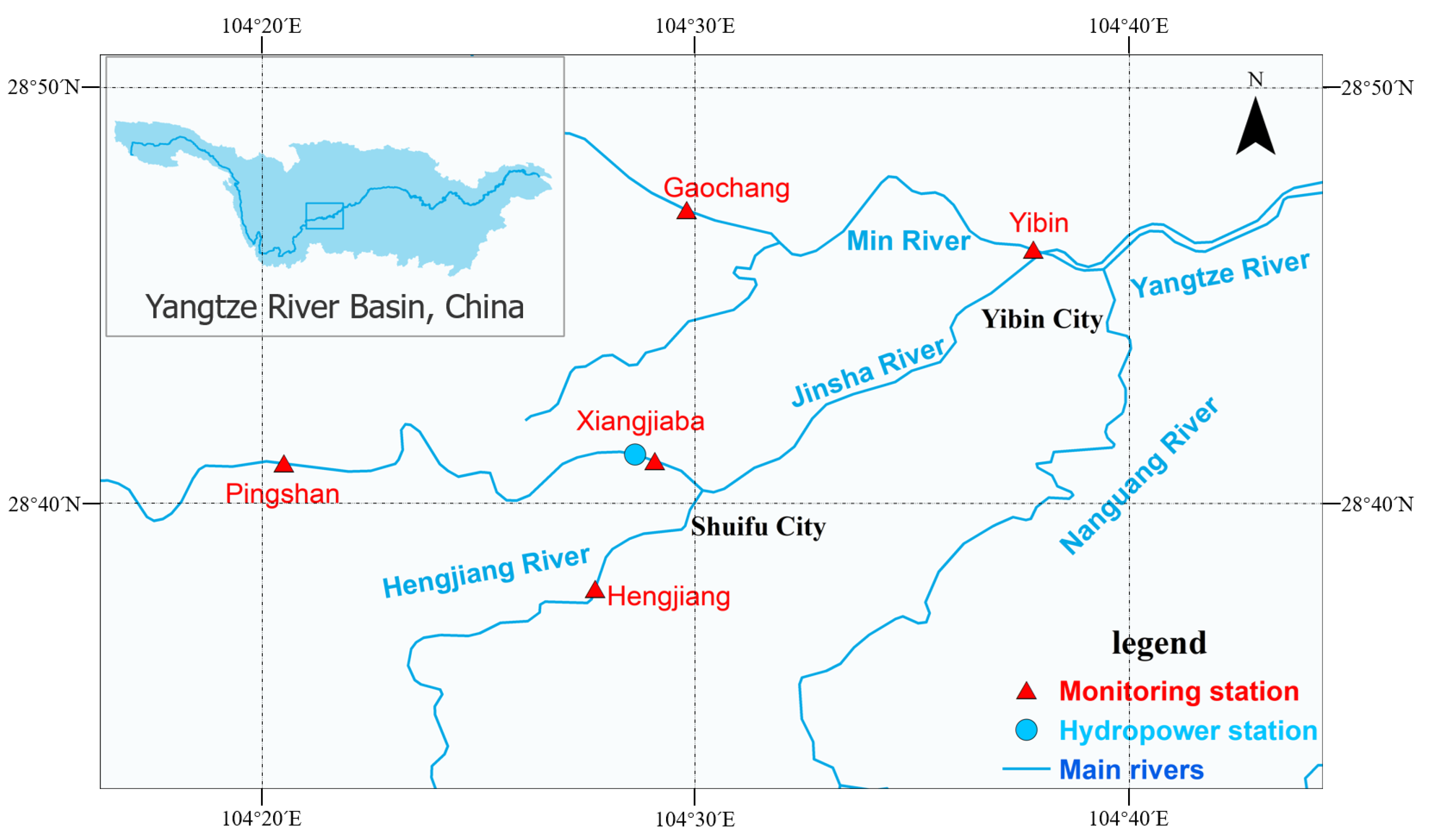
Figure 1.
Distribution map of main dams (blue circle) and hydrological monitoring points (red triangles) in the study area.
Figure 1.
Distribution map of main dams (blue circle) and hydrological monitoring points (red triangles) in the study area.
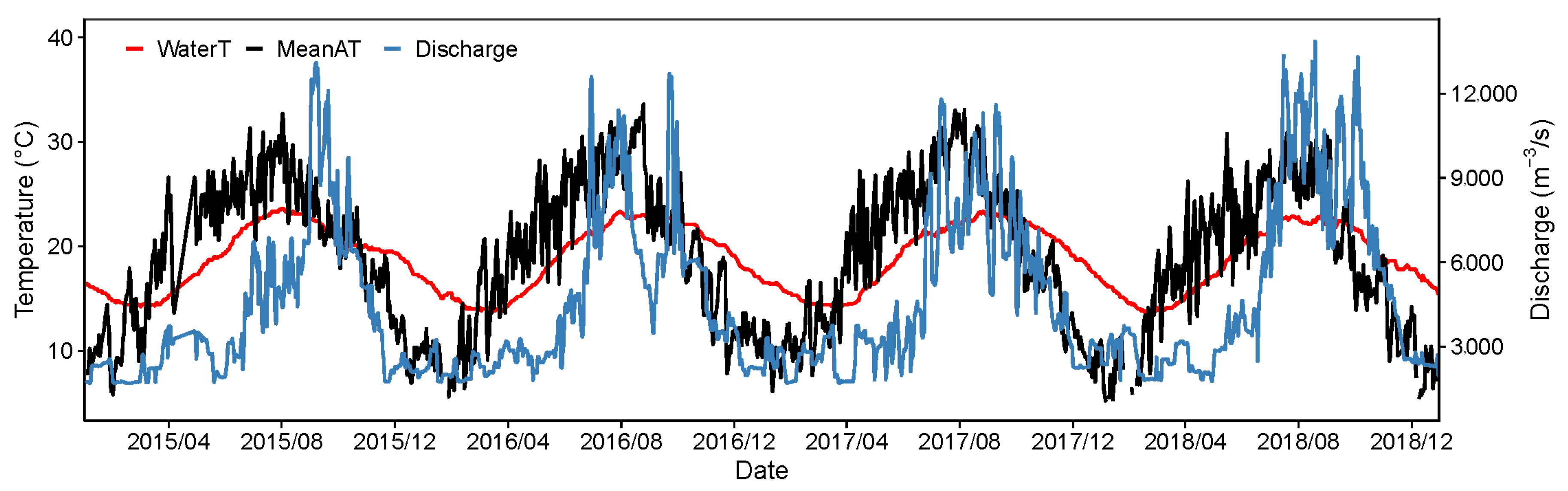
Figure 2.
Time series plot of water temperature (red lines), mean air temperature (black lines), and discharge (blue lines).
Figure 2.
Time series plot of water temperature (red lines), mean air temperature (black lines), and discharge (blue lines).
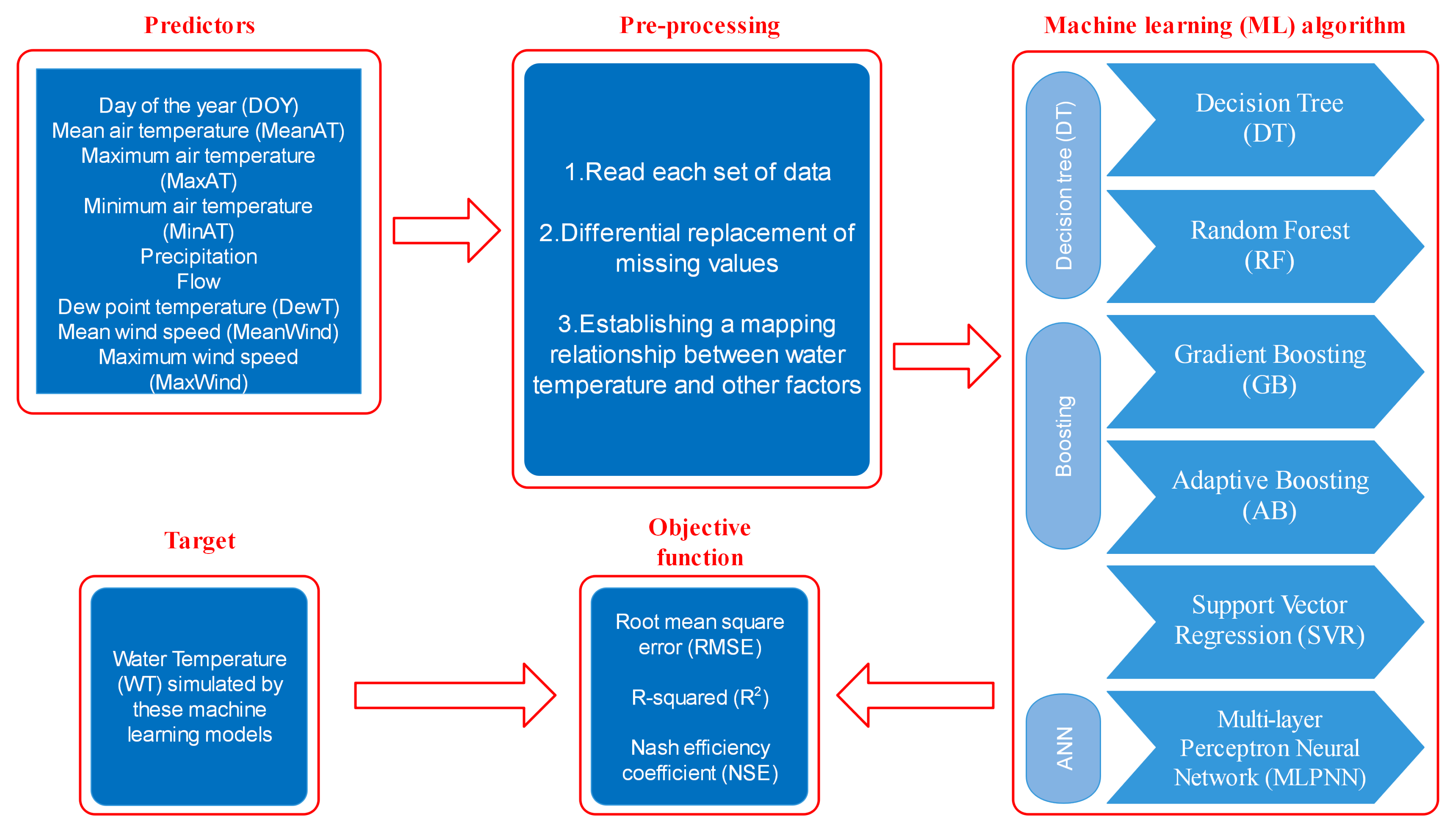
Figure 3.
Workflow summarizing the steps of the comparative analysis of the performance of the different ML methods.
Figure 3.
Workflow summarizing the steps of the comparative analysis of the performance of the different ML methods.
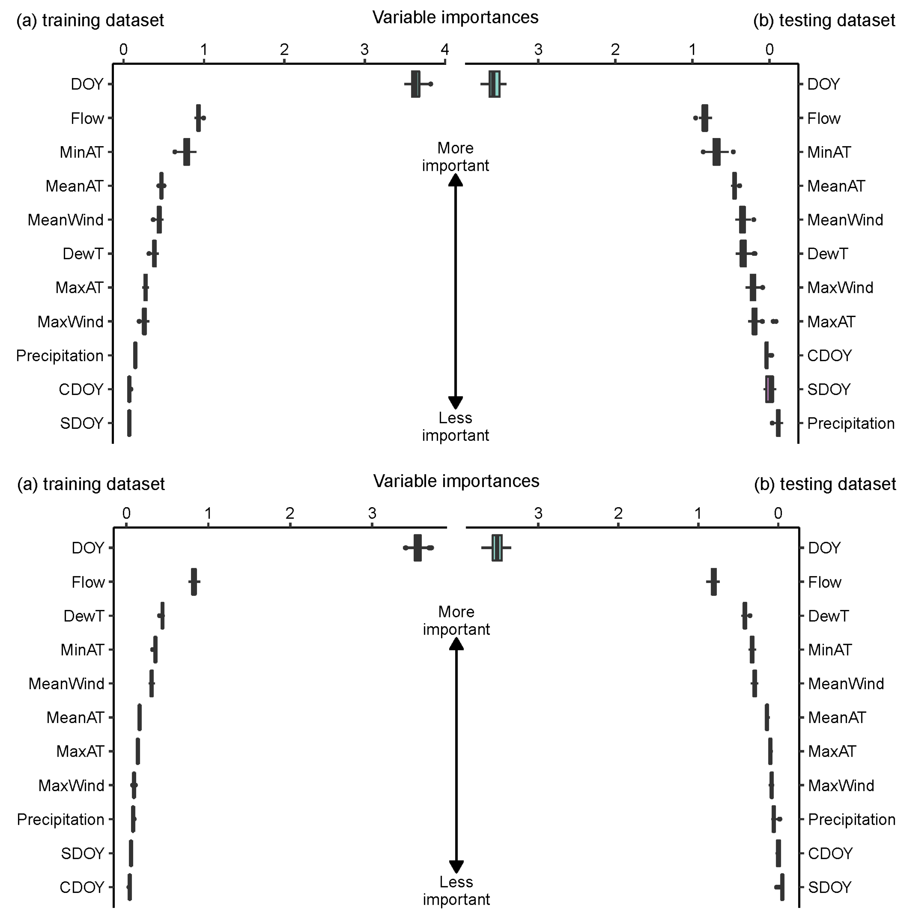
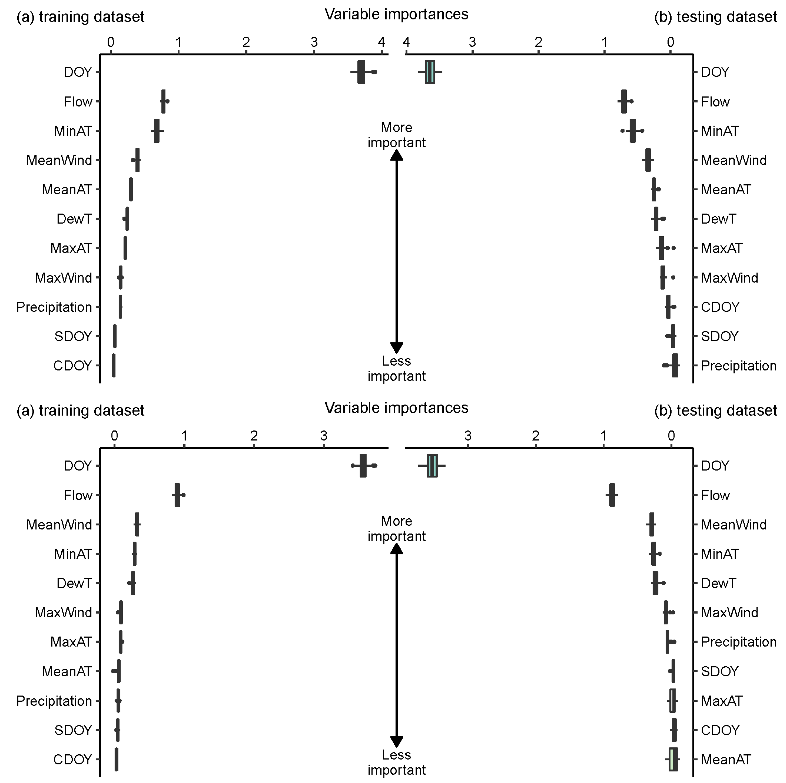
Figure 4.
Permutation importance in DT and RF; DT, decision trees, RF, random forests. (DT on the top, RF on the bottom, WT: °C).
Figure 4.
Permutation importance in DT and RF; DT, decision trees, RF, random forests. (DT on the top, RF on the bottom, WT: °C).
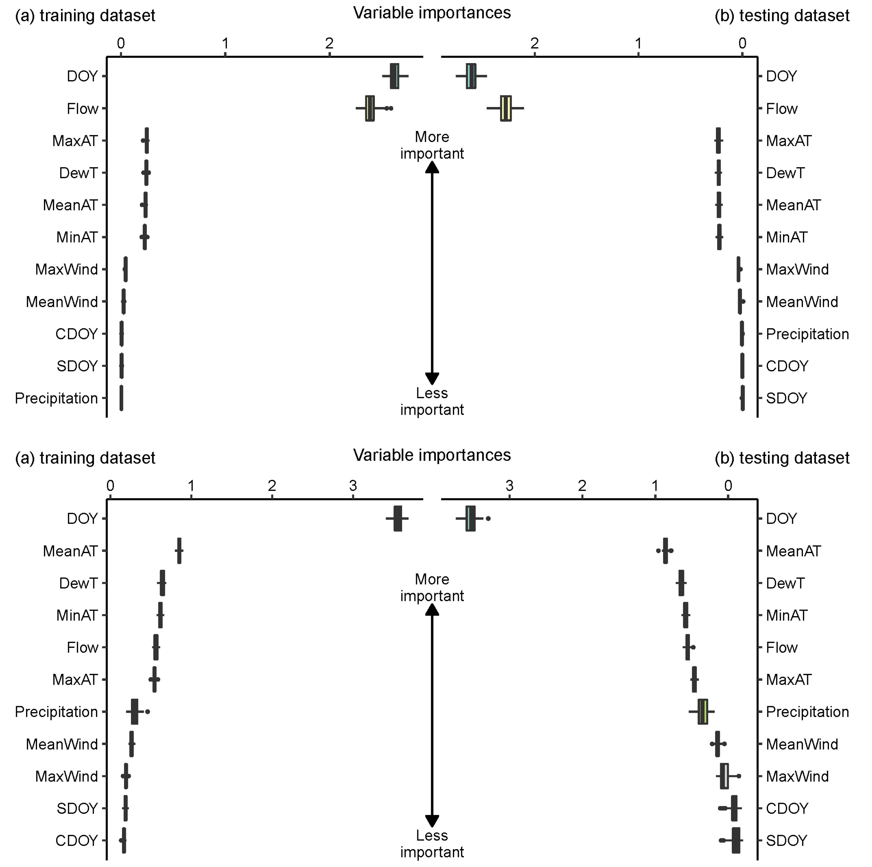
Figure 5.
Permutation importance in GB and AB; GB, gradient boosting regression, AB, adaptive boosting regression. (GB on the top, AB on the bottom, WT: °C).
Figure 5.
Permutation importance in GB and AB; GB, gradient boosting regression, AB, adaptive boosting regression. (GB on the top, AB on the bottom, WT: °C).
Figure 6.
Permutation importance in SVR and MLPNN; SVR, support vector regression, MLPNN, multilayer perceptron neural networks. (SVR on the top, MLPNN on the bottom, WT: °C).
Figure 6.
Permutation importance in SVR and MLPNN; SVR, support vector regression, MLPNN, multilayer perceptron neural networks. (SVR on the top, MLPNN on the bottom, WT: °C).
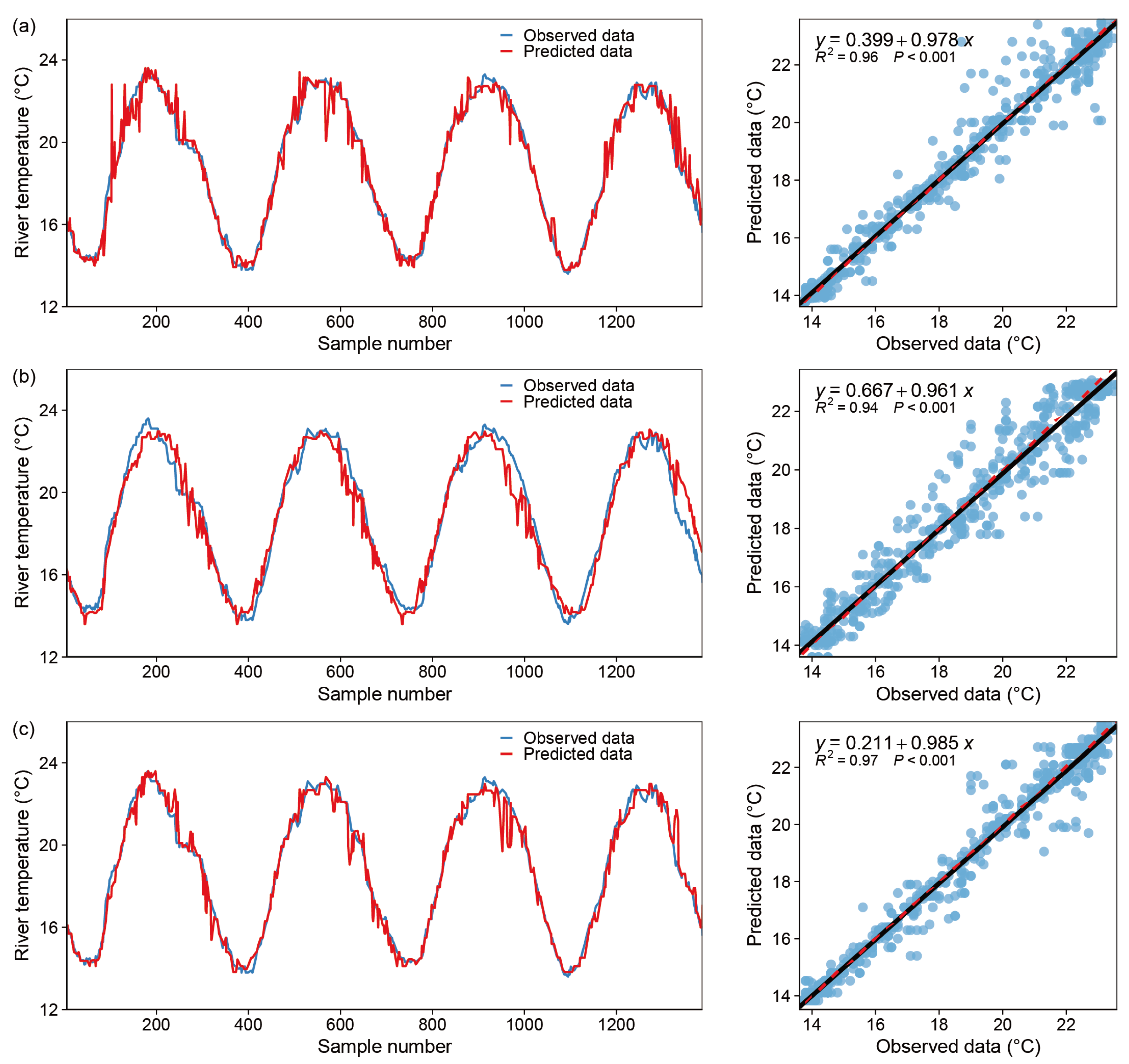
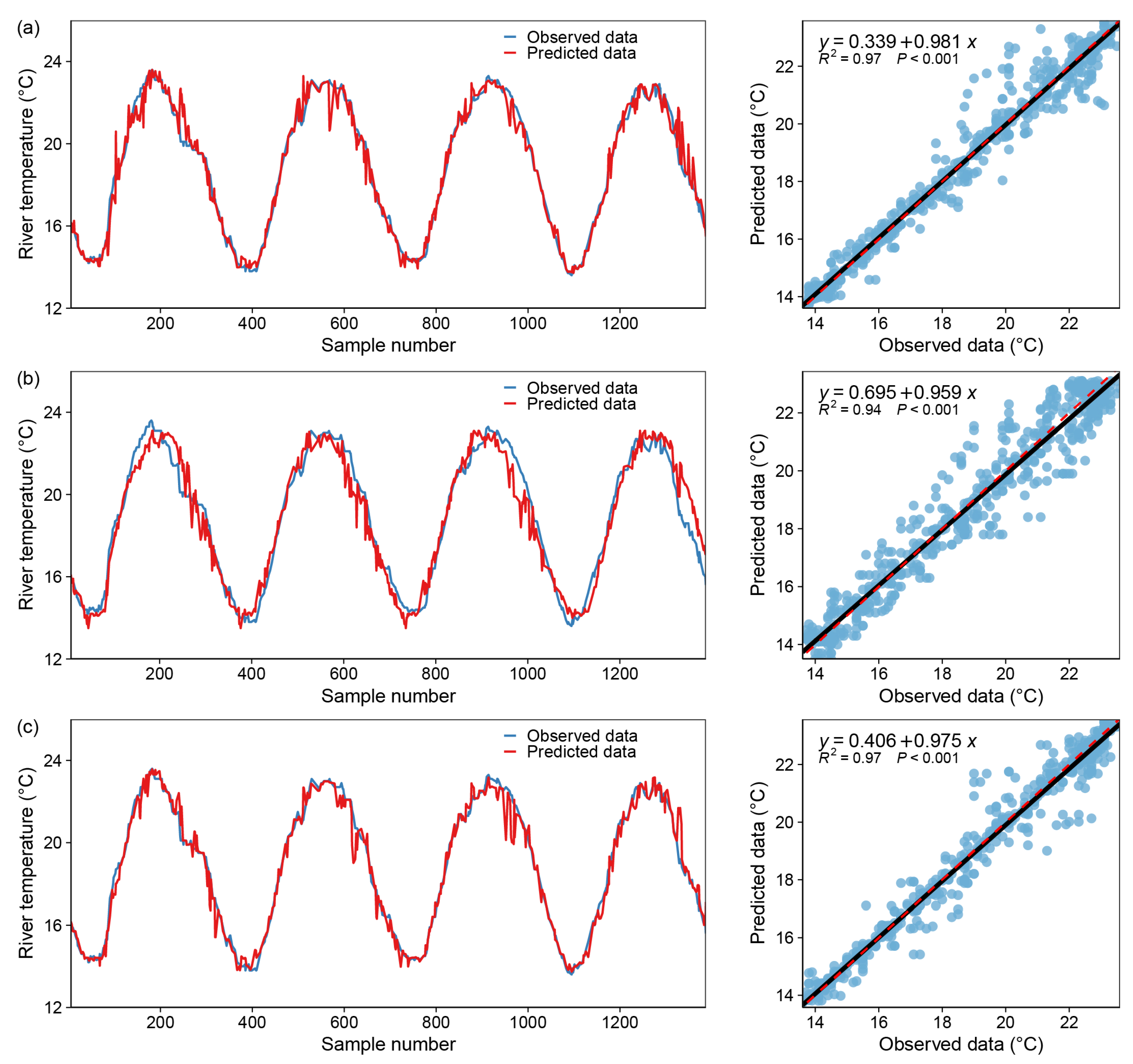
Figure 7.
Model fitting results—DecisionTree Regressor, blue dot: X coordinate (observed data), Y coordinate (predicted data); black line: y = x; red dotted line: the regression curve of the blue dots. (a) only one input variable (DOY), (b) two input variables (DOY and Flow), (c) all variables.
Figure 7.
Model fitting results—DecisionTree Regressor, blue dot: X coordinate (observed data), Y coordinate (predicted data); black line: y = x; red dotted line: the regression curve of the blue dots. (a) only one input variable (DOY), (b) two input variables (DOY and Flow), (c) all variables.
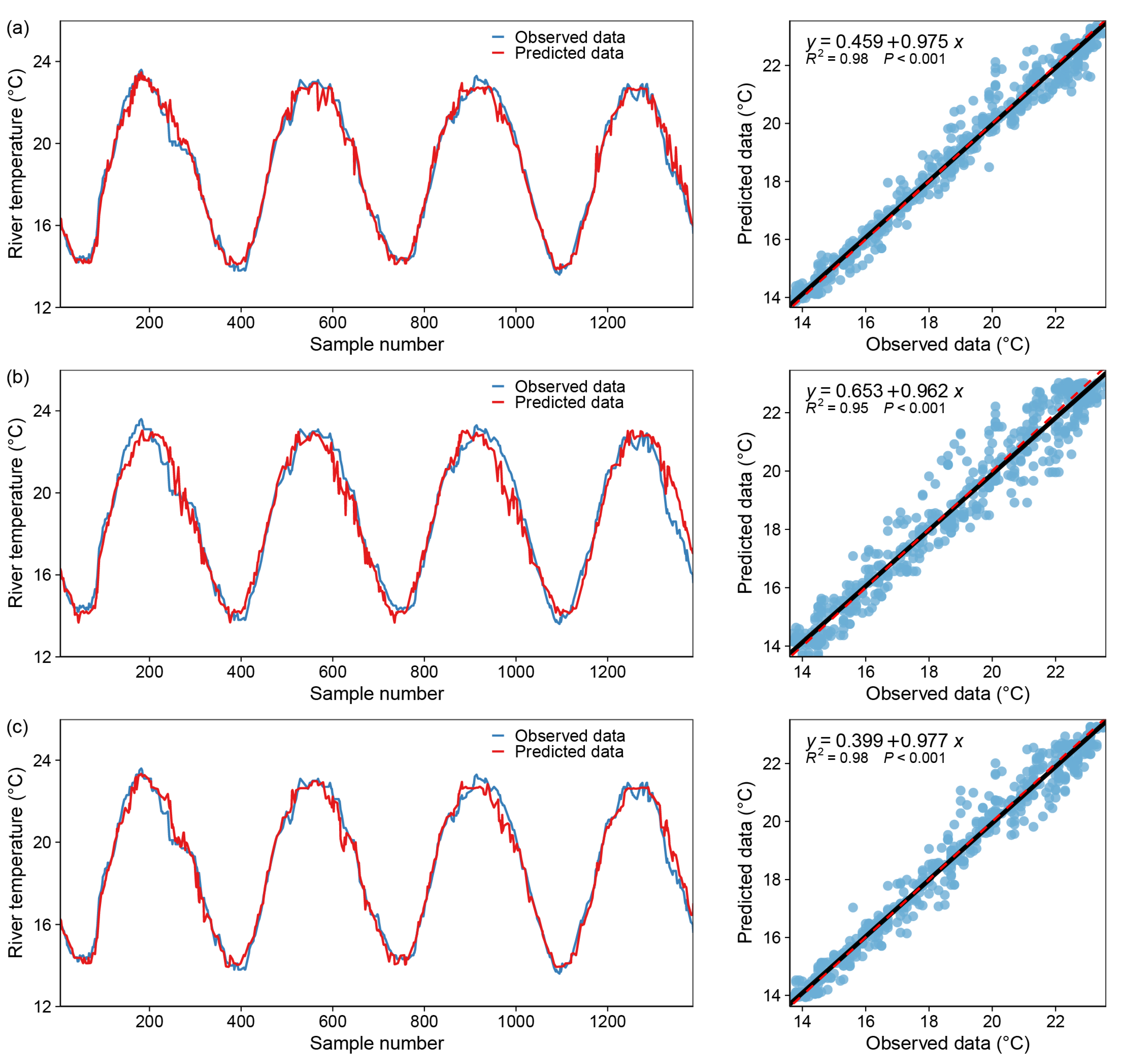
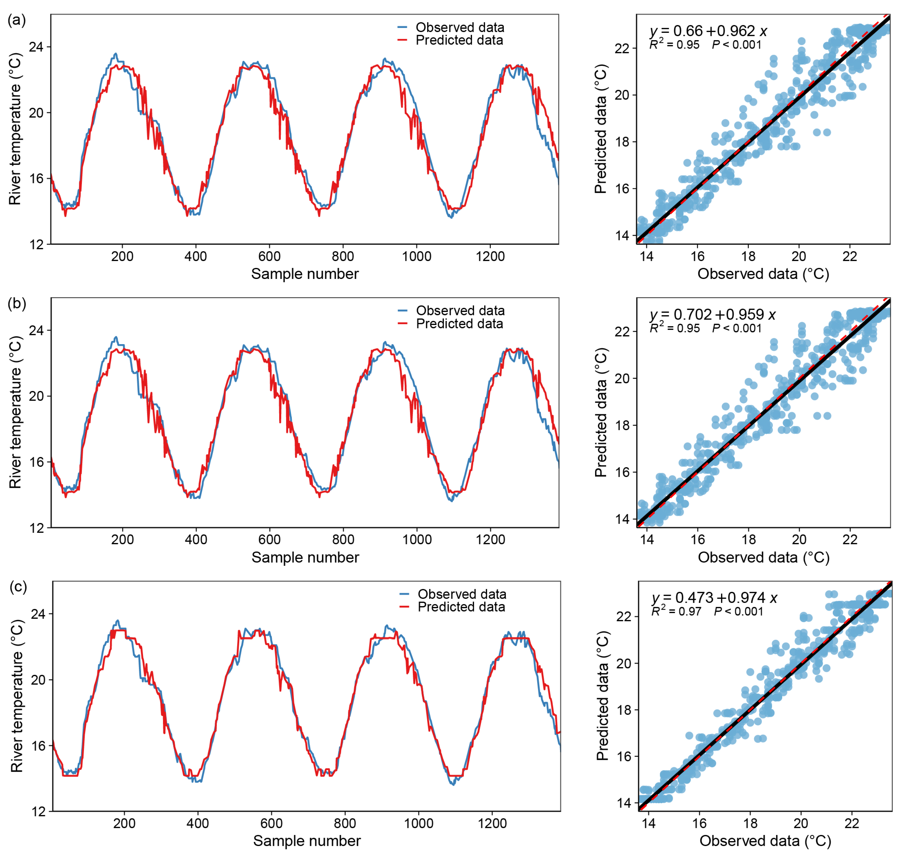
Figure 8.
Model fitting results—RandomForest Regressor, blue dot: X coordinate (observed data), Y coordinate (predicted data); black line: y = x; red dotted line: the regression curve of the blue dots. (a) only one input variable (DOY), (b) with two input variables (DOY and Flow), (c) with all variables.
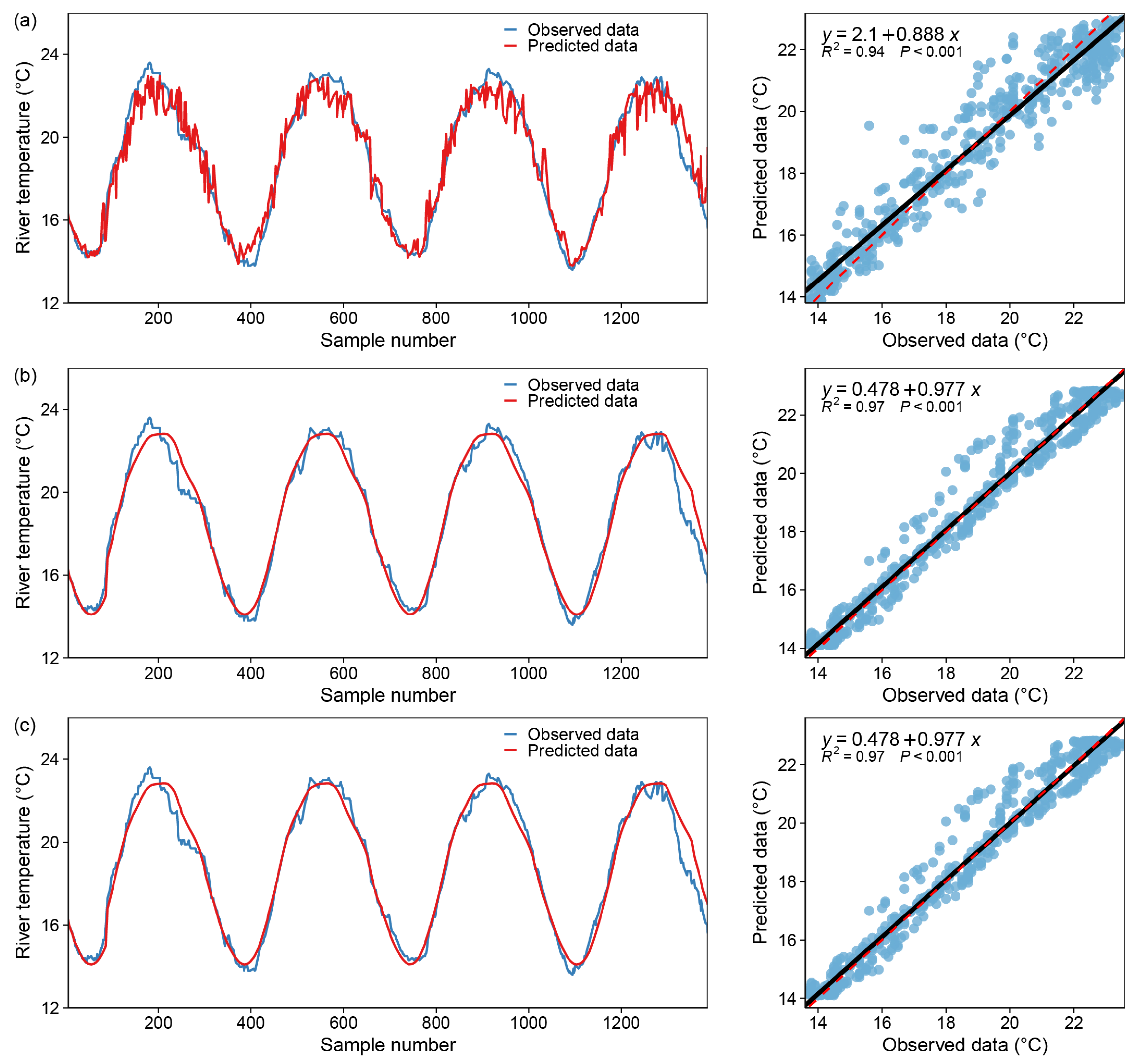
Figure 9.
Model fitting results—GradientBoosting Regressor, blue dot: X coordinate (observed data), Y coordinate (predicted data); black line: y = x; red dotted line: the regression curve of the blue dots. (a) only one input variable (DOY), (b) with two input variables (DOY and Flow), (c) with all variables.
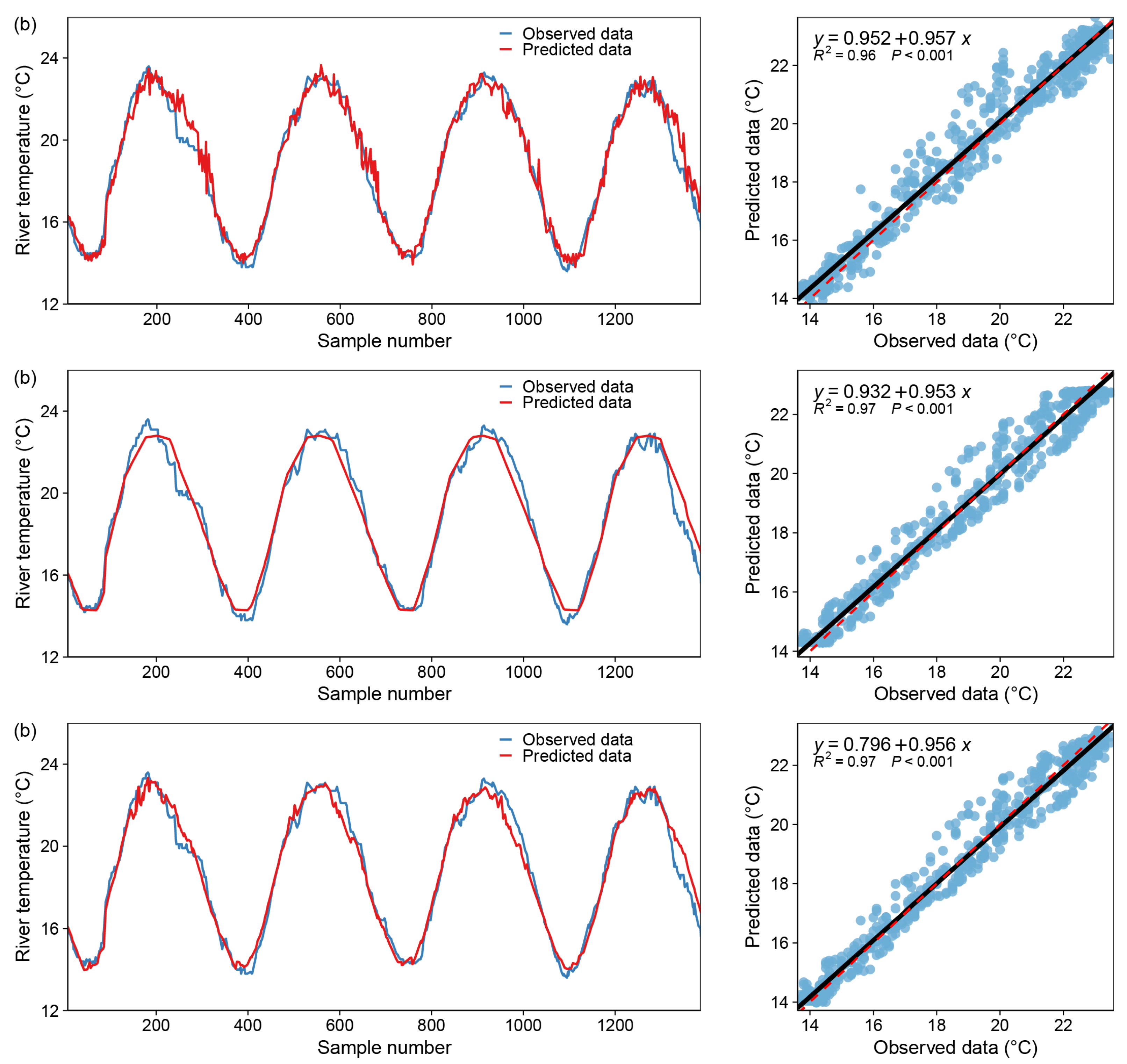
Figure 10.
Model fitting results—AdaptiveBoosting Regressor, blue dot: X coordinate (observed data), Y coordinate (predicted data); black line: y = x; red dotted line: the regression curve of the blue dots. (a) only one input variable (DOY), (b) with two input variables (DOY and Flow), (c) with all variables.
Figure 11.
Model fitting results—SupportVector Regression, blue dot: X coordinate (observed data), Y coordinate (predicted data); black line: y = x; red dotted line: the regression curve of the blue dots. (a) only one input variable (DOY), (b) with two input variables (DOY and Flow), (c) with all variables.
Figure 12.
Model fitting results—Multilayer Perceptron Neural Network, blue dot: X coordinate (observed data), Y coordinate (predicted data); black line: y = x; red dotted line: the regression curve of the blue dots. (a) only one input variable (DOY), (b) with two input variables (DOY and Flow), (c) with all variables.
Table 1.
Performances of six models (DT: decision trees, RF: random forests, GB: gradient boosting regression, AB: adaptive boosting regression, SVR: support vector regression, MLPNN: multilayer perceptron neural networks) in predicting water temperature.
Table 1.
Performances of six models (DT: decision trees, RF: random forests, GB: gradient boosting regression, AB: adaptive boosting regression, SVR: support vector regression, MLPNN: multilayer perceptron neural networks) in predicting water temperature.
| Models | Training Datasets | Testing Datasets |
|---|
| RMSE (°C) | R2 | NSE | RMSE (°C) | R2 | NSE |
|---|
| DT | 0.0167698 | 0.998298 | 0.998295 | 0.394039 | 0.959443 | 0.959352 |
| RF | 0.0513479 | 0.994788 | 0.994694 | 0.203134 | 0.979092 | 0.978487 |
| GB | 2.59 × 10⁻¹⁹ | 1 | 1 | 0.308065 | 0.968292 | 0.968119 |
| AB | 0.0980462 | 0.990049 | 0.989885 | 0.264675 | 0.972758 | 0.972145 |
| SVR | 0.3365923 | 0.965837 | 0.960535 | 0.633647 | 0.934781 | 0.922508 |
| MLPNN | 0.1896209 | 0.980754 | 0.980438 | 0.385593 | 0.960312 | 0.958261 |
Table 2.
Performances of DecisionTree Regressor in modeling water temperature (WT: °C), DT1: only one input variable (DOY), DT2: with two input variables (DOY and Flow), DT3: with all input variables.
Table 2.
Performances of DecisionTree Regressor in modeling water temperature (WT: °C), DT1: only one input variable (DOY), DT2: with two input variables (DOY and Flow), DT3: with all input variables.
| Model Version | Training Dataset | Test Dataset |
|---|
| RMSE (°C) | R2 | NSE | RMSE (°C) | R2 | NSE |
|---|
| DT1 | 0.200361 | 0.979664 | 0.979242 | 0.553881 | 0.942991 | 0.941738 |
| DT2 | 0.043619 | 0.995573 | 0.995553 | 0.329739 | 0.966061 | 0.966209 |
| DT3 | 0.01677 | 0.998298 | 0.998295 | 0.359478 | 0.963 | 0.962799 |
Table 3.
Performances of RandomForest Regressor in modeling water temperature (WT: °C), RF1: only one input variable (DOY), RF2: with two input variables (DOY and Flow), RF3: with all input variables.
Table 3.
Performances of RandomForest Regressor in modeling water temperature (WT: °C), RF1: only one input variable (DOY), RF2: with two input variables (DOY and Flow), RF3: with all input variables.
| Model Version | Training Dataset | Test Dataset |
|---|
| RMSE (°C) | R2 | NSE | RMSE (°C) | R2 | NSE |
|---|
| RF1 | 0.200538 | 0.979646 | 0.979199 | 0.485061 | 0.950074 | 0.948793 |
| RF2 | 0.100807 | 0.989769 | 0.989547 | 0.23512 | 0.9758 | 0.975281 |
| RF3 | 0.051348 | 0.994788 | 0.994694 | 0.203134 | 0.979092 | 0.978487 |
Table 4.
Performances of GradientBoosting Regressor in modeling water temperature (WT: °C), GB1: only one input variable (DOY), GB2: with two input variables (DOY and Flow), GB3: with all inputs variable.
Table 4.
Performances of GradientBoosting Regressor in modeling water temperature (WT: °C), GB1: only one input variable (DOY), GB2: with two input variables (DOY and Flow), GB3: with all inputs variable.
| Model Version | Training Dataset | Test Dataset |
|---|
| RMSE (°C) | R2 | NSE | RMSE (°C) | R2 | NSE |
|---|
| GB1 | 0.194251 | 0.980284 | 0.979888 | 0.584754 | 0.939813 | 0.938425 |
| GB2 | 0.000596 | 0.99994 | 0.999939 | 0.302442 | 0.968871 | 0.968273 |
| GB3 | 2.59 × 10⁻¹⁹ | 1 | 1 | 0.308065 | 0.968292 | 0.968119 |
Table 5.
Performances of AdaptiveBoosting Regressor in modeling water temperature (WT: °C), AB1: only one input variable (DOY), AB2: with two input variables (DOY and Flow), AB3: with all inputs variable.
Table 5.
Performances of AdaptiveBoosting Regressor in modeling water temperature (WT: °C), AB1: only one input variable (DOY), AB2: with two input variables (DOY and Flow), AB3: with all inputs variable.
| Model Version | Training Dataset | Test Dataset |
|---|
| RMSE (°C) | R2 | NSE | RMSE (°C) | R2 | NSE |
|---|
| AB1 | 0.202579 | 0.979439 | 0.978967 | 0.535933 | 0.944838 | 0.943332 |
| AB2 | 0.15983 | 0.983778 | 0.983445 | 0.291648 | 0.969982 | 0.969293 |
| AB3 | 0.20119 | 0.97958 | 0.979129 | 0.538943 | 0.944528 | 0.943291 |
Table 6.
Performances of SupportVector Regression in modeling water temperature (WT: °C), SVR1: only one input variable (DOY), SVR2: with two input variables (DOY and Flow), SVR3: with all input variables.
Table 6.
Performances of SupportVector Regression in modeling water temperature (WT: °C), SVR1: only one input variable (DOY), SVR2: with two input variables (DOY and Flow), SVR3: with all input variables.
| Model Version | Training Dataset | Test Dataset |
|---|
| RMSE (°C) | R2 | NSE | RMSE (°C) | R2 | NSE |
|---|
| SVR1 | 0.288101 | 0.970759 | 0.970421 | 0.323232 | 0.966731 | 0.966283 |
| SVR2 | 0.34541 | 0.964942 | 0.959725 | 0.630718 | 0.935082 | 0.923919 |
| SVR3 | 0.336592 | 0.965837 | 0.960535 | 0.633647 | 0.934781 | 0.922508 |
Table 7.
Performances of Multilayer Perceptron Neural Network in modeling water temperature (WT: °C), MLPNN1: only one input variable (DOY), MLPNN2: with two input variables (DOY and Flow), MLPNN3: with all input variables.
Table 7.
Performances of Multilayer Perceptron Neural Network in modeling water temperature (WT: °C), MLPNN1: only one input variable (DOY), MLPNN2: with two input variables (DOY and Flow), MLPNN3: with all input variables.
| Model Version | Training Dataset | Test Dataset |
|---|
| RMSE (°C) | R2 | NSE | RMSE (°C) | R2 | NSE |
|---|
| MLPNN1 | 0.274755 | 0.972113 | 0.970939 | 0.311318 | 0.967957 | 0.965799 |
| MLPNN2 | 0.236238 | 0.976023 | 0.975322 | 0.280818 | 0.971096 | 0.969259 |
| MLPNN3 | 0.189621 | 0.980754 | 0.980438 | 0.385593 | 0.960312 | 0.958261 |
Table 8.
Best version of performance in different models (DT: decision trees, RF: random forests, GB: gradient boosting regression, AB: adaptive boosting regression, SVR: support vector regression, and MLPNN: multilayer perceptron neural networks) in predicting water temperature (WT: °C), 1.only one input variable (DOY), 2. with two input variables (DOY and Flow), 3. with all variables.
| Training Dataset | Test Dataset |
|---|
| Models | RMSE (°C) | R2 | NSE | Models | RMSE (°C) | R2 | NSE |
| DT3 | 0.017 | 0.998 | 0.998 | DT2 | 0.330 | 0.966 | 0.966 |
| RF3 | 0.051 | 0.995 | 0.995 | RF3 | 0.203 | 0.979 | 0.978 |
| GB3 | 2.6 × 10⁻¹⁹ | 1.000 | 1.000 | GB2 | 0.302 | 0.969 | 0.968 |
| AB2 | 0.160 | 0.984 | 0.983 | AB2 | 0.292 | 0.970 | 0.969 |
| SVR1 | 0.288 | 0.971 | 0.910 | SVR1 | 0.323 | 0.967 | 0.966 |
| MLPNN3 | 0.190 | 0.981 | 0.980 | MLPNN2 | 0.281 | 0.971 | 0.969 |


