Abstract
Municipal water mains are built with a target service age of several decades. In such a long life, breaks can occur, even multiple times. Water mains can be maintained before or right at breaks. The former is referred to as the preventive strategy, whereas the latter is the corrective strategy. Depending on the costs of repair, replacement, and failure consequence, different strategies should typically be implemented in order to achieve the optimal watermain management in terms of life cycle costs. This study aims to investigate the optimal scenarios for the two strategies based on a two-time-scale (TTS) point process used to model the deterioration of water mains. The corrective strategy is to determine the optimal number , where upon the -th break, implementing a replacement for water main is justified, compared to a minimal repair. The preventive strategy is to determine the optimal replacement time in terms of pipe survival probability . Monte Carlo simulations are used to investigate the optimal and considering a number of influential factors, including model parameters of the intensity function and ratios of maintenance, replacement, and consequence costs. Then, the full distributions of the life cycle costs are characterized with the mean of total life cycle costs being the target for optimization. Last, a case study is illustrated to demonstrate the application of both strategies in real water systems. An important finding is that with a typical pipe diameter of 400 mm and length of 200 m, the optimal is typically less than five, and the optimal is below 50%.
1. Introduction
Water mains are key municipal infrastructure assets supporting the daily life of citizens [1]. Though water mains are designed to serve for several decades, they deteriorate with increasing service age, and can break before reaching the target design life. As a matter of fact, unexpected water main breaks are very common in reality. A main reason is that water mains are buried underground, and thus, it is very difficult to inspect and monitor their service conditions nondestructively, non-disruptively, timely, and easily [2,3].
Upon a water main break, municipal water managers have to decide whether to repair or replace the pipe. Even for water mains installed at some critical areas where a failure would cause severe loss, a preventive strategy can be adopted. A corrective strategy means maintaining a water main only after breaks occur, whereas a preventive strategy refers to maintaining a water main before it breaks.
Usually, if the consequence of failure is of little concern, maintenance can be implemented after a failure takes place. On the other end, if the failure would bring about massive loss [4,5], then a preventive strategy is warranted. Other than these two extreme cases, how to optimize the managing strategies depends on a set of influencing factors, for example, deterioration of the mains, repair cost, replacement cost, consequence, readiness of repairing technology, pipe location, ease of access, municipal budget, citizen affordability upon break, flooding risk, etc.
Although advanced managing strategies such as multiple target optimization on water pipe network level have been advocated [6,7], the application seems still limited in local areas due to the complexity. The current practice is still based on a ‘fire-fighting’ strategy coupled with a service age strategy, for example, replacing a pipe when the service age reaches 40 years regardless of its conditions. Moreover, the threshold service age at which a pipe will be replaced is selected somewhat arbitrarily, and with a lack of sound evidence. Obviously, improvements can be made.
This study investigates the optimization of managing strategies for water mains by setting the minimization of life cycle cost as the target. To do this, a proper deterioration model capturing breaks of water mains must be first determined. On the one hand, repairing a broken water main minimally will no doubt resume its functionality; however, the pipe condition remains the same, or at least not significantly improved, and degradation continues as before. A drawback for minimal repair, although it costs less, is that the water main could break again shortly after treatment. If so, another repair is then needed. Continuous repairs add up to the maintenance cost. On the other hand, replacing a broken water main with a new one starts a new life cycle. The new main is in excellent condition, and can be expected to serve for a much longer time before a break takes place. Nevertheless, a replacement typically costs much more than that of a minimal repair. Despite extensive studies on the management and maintenance of infrastructure assets, e.g., van Noortwijk [8], van Noortwijk and Frangopol [9], Jardine and Tsang [10], Bull [11], and Campbell et al. [12], under which scenarios a water main should be replaced rather than repaired remains a question to answer.
As a matter of fact, the estimation of the life cycle cost of water mains depends significantly on the deterioration. There have been extensive deterioration models proposed for water pipes, e.g., both break-history-independent [13,14,15,16,17,18,19,20] and -dependent [21,22,23]. Reviews of the modelling of water pipe deterioration can be seen in [2,24,25,26,27,28]. Obviously, history independence is a strong assumption in the prediction of water main breaks, which will inevitably reduce the prediction accuracy. As such, degradation models considering the breaking histories are superior and advantageous to be adopted in life cycle costing analysis (LCCA). Nevertheless, this is the part that has not yet received due attention in the current literature for the life cycle management of municipal water pipe networks. Existing studies, though they have made significant advances in water pipe management, have focused largely upon network effects and a simplification of methods for LCCA, e.g., Termes-Rifé et al. [29], Roshani and Filion [30], Naoum-Sawaya et al. [31], Lee et al. [32], Ghobadi et al. [33], among other excellent works. A brief review of LCCA for water pipes can be found in Ghobadi et al. [33].
In this paper, we examine two simple maintenance and replacement strategies for water mains. The first is a corrective strategy which is to determine the optimal number of breaks at which the water main is replaced; before reaching the -th break, repair is implemented upon a break. The second is a preventive strategy, which is to determine the optimal survival probability at which the water main is replaced. The water main break, along with time, is modelled as a two-time-scale (TTS) point process, proposed by Lin and Yuan [34]. The influences of degradation intensity, ratios of maintenance, replacement, and failure consequence costs are discussed. The Monte Carlo simulation approach is adopted to conduct the analyses. A case study is provided in the end to elaborate the application of the two strategies for the real world. The outcomes of this study are valuable to municipalities for implementing better management strategies for water mains.
The rest of the paper is organized as follows. The next section introduces the TTS degradation model for water mains and the simulation technique for breaks. The definition of life cycle cost is formulated in Section 3 with respect to corrective and preventive strategies. Section 4 shows the results of strategy optimization, followed by a case study in Section 5. The paper is concluded in Section 6, followed by references.
2. Degradation Model
2.1. Modelling Water Main Breaks as a Point Process
Upon a break, a water main is not always replaced by a new one; instead, it is usually repaired, which brings the main back to functioning. Since the working conditions, e.g., surrounding soils, inner pressure, corrosion, external loading, etc., are typically unknown or just partially known, physical modeling of the birth and growth of defects on a pipe turns out to be very challenging, if not impossible [35]. An alternative is to model the occurrence of a water main break phenomenically [36]. If ordering all water main breaks in terms of breaking times, then a series of ‘points’ in the timeline are obtained, as shown in Figure 1. Due to the unknown, the occurrence of these points is uncertain. This can then be simply modelled as a stochastic point process.
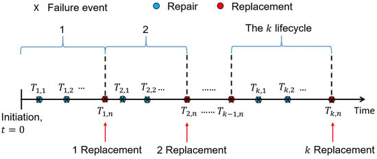
Figure 1.
Concept of modelling failure events as a point process.
For a simple point process, it can be fully characterized by a conditional intensity function describing the potential of an event to take place within the next interval of time given the event history. According to Cox and Isham [37] and Cook and Lawless [38], the conditional intensity can be mathematically expressed as:
where = history of the until before time ; and is the number of occurrences within the time interval . where . When approaches zero, the probability for more than one event to occur within the period is ignorable. This assumption can be written as . Discussion on the general theory of point processes in detail can be found in Cox and Isham [37], Jacobsen [39], Cook and Lawless [38], and Daley and Vere-Jones [40], among others.
2.2. The Two-Time-Scale (TTS) Intensity Function
The break of water mains has been most commonly modelled as a Poisson process. An implicit assumption of this type of modelling is that breaks to occur do not depend on the breaking history. Nevertheless, this is a strong assumption and does not have any solid scientific support. To account for the influence of breaking history upon the future breaks, Lin and Yuan [34] developed a two-time-scale (TTS) intensity function for breaks of water mains. The intensity function includes an overall time scale representing the entire pipe deterioration, as well as a local time scale representing the renewal effect. The TTS function is expressed as:
where = current time; = sojourn time since the last break; , , and are model parameters. Obviously, the break history in Equation (2) is simplified as inter-occurrence duration .
Lin and Yuan [34] demonstrated the capability of the TTS model in capturing different deterioration trends, i.e., both monotonic and non-monotonic. In particular, it is able to model a bathtub curve deteriorating trend, which is of great interest to engineers, as shown in Figure 2, where the surface of is plotted against model parameter and the sojourn time given , , , and . Note that these values for , , and are intentionally selected here for to be in a bathtub curve shape, which is a highly desirable deterioration trend for engineers to model. With an increase in the sojourn time from zero, the intensity first drops dramatically until reaching a minimal, then increases back as continues to increase. The parameter controls the overall scale of , whereas and are the shape factors controlling the trend together. With the increasing of , first decreases to a minimum and then increases, showing a bathtub curve. Table 1 summarizes the trends that correspond to the permutations of and . In general, the larger the , the higher the breaking potential of a water main. Readers are directed to Lin and Yuan [34] for more explorations on Equation (2).
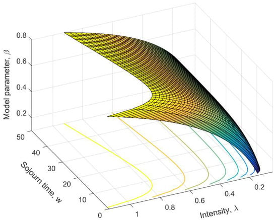
Figure 2.
Three-dimensional plot of against model parameter and the sojourn time given , , , and .

Table 1.
Summary of deterioration trends captured by the TTS model with respect to permutations of model parameters (after Lin and Yuan [34]).
2.3. Simulating a TTS Point Process
Given , the probability of a water main surviving through a time duration [,] can be computed as [38,41]:
Equation (3) suggests that once , , and are known, can be determined by solving the equation. Based on the breaking data in the city of Toronto, Canada, Lin and Yuan [34] showed that the TTS is superior to Poisson process, and water mains follow a bathtub deterioration trend. Therefore, the TTS intensity function is adopted here, and the model parameters are taken as , , and for analyses. Figure 3 shows 100 simulated TTS point processes starting from . For the simulations, is randomly sampled from a uniform distribution of .
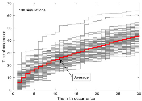
Figure 3.
Simulated water main breaking events using the TTS point process model assuming , , and .
On average, the first two breaks occur within , i.e., , . A total of eight breaks can be expected within . It should be noted that here, does not have a unit, meaning that it can be a year, month, minute, second, or others, depending on the data used for investigation. Another observation is that the simulated break events tend to occur either one shortly after another, or none within a relatively long period of time. This matches observations from engineering experience.
3. Definition of Life Cycle Cost
Upon a break, a water main pipe can be either maintained or replaced. Maintenance resumes the serviceability of the main while the deterioration continues at the original rate [42,43,44]. On the other hand, a replacement brings in a new main pipe and starts a new life cycle. Suppose the cost of a maintenance is and the cost of a replacement is ; then, it is reasonable to assume , especially when the no-dig technology is employed [45,46,47,48,49]. In addition to and , failure consequence is another primary source of costs. For example, a water main break could block the traffic for hours, flooding infrastructure assets, and thus, resulting in damage and loss. The cost due to failure consequence is denoted as in this study. Depending on , , , and , different strategies must be practiced to reach the goal of minimum life cycle cost for water main asset management. Two asset management approaches are considered here: corrective and preventive strategies. The following introduces these two strategies, including the definition of life cycle cost and the steps to compute these costs.
3.1. Corrective Strategy
A corrective strategy is that the maintenance, repair, or replacement is implemented only after water main breaks take place. The cost for each break event is either for maintenance or for replacement. As was pointed out earlier in this paper, a repair or maintenance will only resume the serviceability of the main, but does not improve its condition. The degradation is still accelerating with service age, meaning that the water main will break more frequently as time goes. After some point, minimal repair is no longer cost-effective compared to a renewal.
Consider a simple corrective maintenance strategy: replacing the water main with a new one at the -th breaks; then, the question becomes: what is the optimal ? This idea is illustrated in Figure 1. In terms of the concept of net present value, the total cost of the water main due to maintenance and replacement in a sufficient long planning horizon can be written as:
where = number of lifecycles; D = discount factor converting future cost to net present value. Usually, , with d being the discounted rate. The most commonly used discounted rate is 5% annually [50,51]. This study adopts as a reference for analyses.
Assuming , , and are all constant with time, then for convenience, the life cycle cost expressed by Equation (4) can be normalized by as:
Equation (5) indicates that the optimal mainly depends on the cost ratios of and . If , then obviously the main should be replaced at each break. The breaking event becomes a renewal process. This also applies to cases with severe consequence, i.e., . If , then the optimal solution for will depend on the ratio of .
The steps to determine the optimal value are as follows.
Step 1. Determine the values for the ratios of and , discounting factor , and for model parameters , , and ;
Step 2. Select an initial value, e.g., ;
Step 3. Generate a realization of the TTS point process given the pre-determined , , and ;
Step 4. Compute the normalized life cycle cost using Equation (5);
Step 5. Repeat Steps 3 to 4 for a sufficient number of times, i.e., 100,000 times in this paper, to obtain the full distribution of life cycle cost ;
Step 6. Calculate the statistics of , i.e., mean, coefficient of variation;
Step 7. Repeat Steps 2 to 6 to compute the means and COVs of for different values; then, the one that gives minimal mean of is determined as the optimal;
Step 8. Change the values of , , , , , and to investigate their influences on the optimal .
3.2. Preventive Strategy
As will be demonstrated later in this study, for cases with high failure consequence, a corrective strategy might not be adequate, and the life cycle cost can still be further optimized by adopting a preventive strategy, that is, replacing a water main before it fails.
Since the exact time instance for a break to take place is unknown, this study takes the survival probability computed as Equation (3) as a time indicator for taking a replacement action. The idea is illustrated in Figure 4.
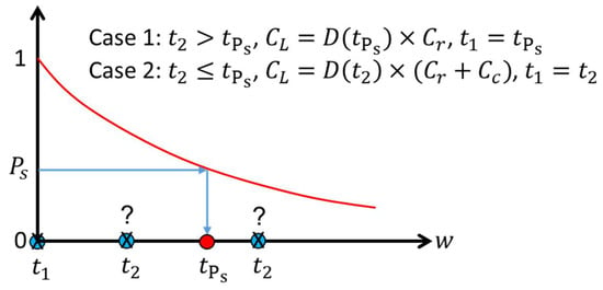
Figure 4.
Illustration of the preventive strategy in terms of survival probability.
Suppose the last break of the water main is at ; then, the steps to compute the cost of the next life cycle are as follows.
Step 1. Select an initial survival probability ;
Step 2. Compute the corresponding using Equation (3);
Step 3. Generate a random sample from a uniform distribution ;
Step 4. Determine corresponding to the with Equation (3);
Step 5. Compare against ; if , then the cost is calculated as , and is updated as ; otherwise, , , and ;
Step 6. Repeat steps 2 to 5 for a large number of times; then sum all the costs up to be the total cost of one simulated path;
Step 7. Repeat Step 6 a large number of times, and take the average as the mean total life cycle cost.
Step 8. Change the initial and repeat steps 2 to 7 until the minimum mean total life cycle cost is reached; then, the corresponding is determined as the optimal .
4. Results of Strategy Optimization
A reference example is firstly set up for analysis purposes: , , , , , and . This setting assumes that the loss due to failure is the same as the cost for a maintenance, whereas the cost of a replacement is 10 times to that of a maintenance. These ratios will be varied to reflect different scenarios, as well as their influences on establishing optimal strategies.
4.1. Corrective Strategy
Figure 5 shows the distributions and the means of the normalized total life cycle costs (in net present value) against the value for the reference example. In the figure, the mean was averaged from 10,000 simulations; each simulation had 1000 cycles. The means, medians, and COVs for the in Figure 5 are summarized in Table 2. As shown, all the distributions are more or less symmetric. Applying K-S tests shows that most of them can be considered normal distributions. The mean is about 30 at , but decreases to about 17.5 as increases to 7; after that, increases to about 22 for . These results suggest that the optimal value is 7, meaning a water main pipe should be replaced by a new one rather than repaired every 7 breaks. The difference of the mean reaches 12.5, i.e., against .
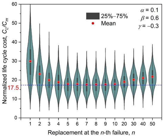
Figure 5.
Normalized life cycle cost varying with replacement at the -th failure (, , and ).

Table 2.
Summary of means, medians, and COVs of the for the example based on the simulations.
Another observation from Figure 5 is that the coefficient of variation (COV) of exhibits a decreasing trend with increasing value. The COV is as large as 32% for the case, and continuously drops to about 22% for the case. It is worth mentioning here that this study takes the mean as the target for life cycle cost optimization. For those taking both mean and COV of as the targets, a different optimal value can be resulted.
It is also worth noting that the mean has a very flat bottom for , varying from 5 to 10. The differences in the mean values are practically negligible. Hence, though the optimal value is , it also seems acceptable to take any integers between 5 and 10 for .
Keeping the other two parameters unchanged while varying the third one for the three TTS model parameters, the effects of , , and on the final outcome of the optimal value are examined. The results are provided in Figure 6. The increases of and lead to a decrease of optimal value, whereas for , the opposite is observed. This can be explained by the fact that both and are parameters acting on the overall level of . The increases of them will result in a higher deterioration intensity, meaning that the water main tends to break more and more frequently. This causes a quick add-up of the total repair cost, and thus, the need of a replacement is justified so as to yield an economic benefit. After replacement, is re-zeroed, and the dramatically drops. Hence, a lower optimal matches better the target of minimizing the total life cycle cost. On the other hand, parameter is a factor acting on the local level of . A smaller (negative value) indicates a stronger local renewal effect of the water main degradation, which, in turn, calls for a more frequent replacement of the asset.
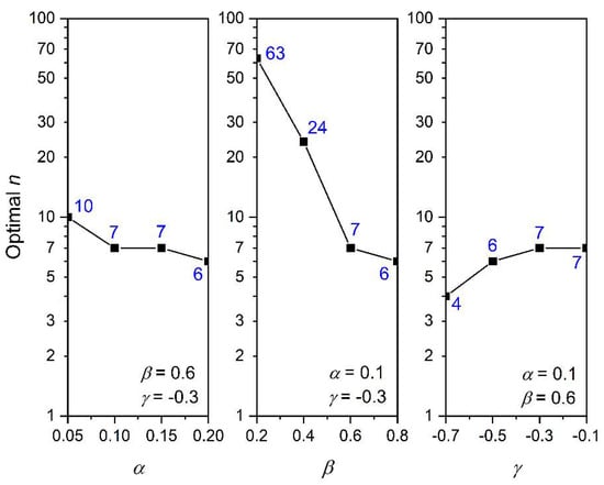
Figure 6.
Effects of the model parameters , , and in the TTS intensity function on the optimal value (, , and ).
The second observation is that the effect of is much larger than those by and . As drops from 0.8 to 0.2, the optimal correspondingly increases from 6 to 63, which is over an order of magnitude of difference. For and , the variation ranges are within 6 to 10 for decreasing from 0.20 to 0.05, and 4 to 7 for increasing from −7 to −0.1. This reveals that is the most influential parameter in .
Despite this, it should be emphasized that, in reality, the sojourn time of a break of water mains could be very long, and the cost, after converted to the net present value, would become very small. An indication of this is that the cost ratios and could play a more important role than the three model parameters.
Figure 7 shows the influences of ratios of consequence to maintenance cost and replacement to maintenance cost on the determined optimal value. For , the optimal value will always be 1, regardless of . This is understandable, as a replacement gives a new water main whose condition is better than a repaired one with a certain service age without extra cost. For , a smaller optimal is obtained for a larger . For example, for , the optimal is found to be 14 if , but drops to 1 after exceeds 9. For , its increase will lead to an increase of the optimal value. Given , the optimal value is 1 for , and increases to 4 for . Figure 7 demonstrates the importance of and in the decision-making of maintenance and replacement strategies for water mains. This also implies the need to implement pertinent strategies for water mains located in different areas, e.g., rural, commercial, residential, or industrial areas.
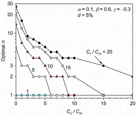
Figure 7.
Influences of ratios of consequence to maintenance cost and replacement to maintenance cost on optimal value.
The last observation from Figure 7 is that it is not uncommon for the optimal value to be 1 under the corrective strategy framework. This suggests implementation of a preventive strategy could be a better solution for those scenarios.
4.2. Preventive Strategy
For preventive strategy, there is no maintenance; only replacement is considered. As a result, is removed from the calculation of life cycle cost ; only and are taken into account. Figure 8 shows the normalized life cycle cost varying with replacement at different survival probabilities of water mains. The means, medians, and COVs for the in Figure 8 are summarized in Table 3. For the scenario of , the optimal survival probability for implementing a replacement is found to be = 70%. The corresponding life cycle cost is . If is increased to 90%, would increase to be about 33.0; if is decreased to 0%, which is equivalent to the corrective strategy of , would increase to be about 32.0. This means that turning the strategy from corrective to preventive, in this case, would reduce the life cycle cost by (32 − 28.2)/32 = 12%. For other cases, the improvement could be larger.
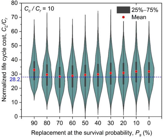
Figure 8.
Normalized life cycle cost varying with replacement at the survival probability of water mains (, , , and ).

Table 3.
Summary of means, medians, and COVs of the for the example based on the simulations.
Similarly, though the mean reaches its minimum at , the COV does not concurrently reach its minimum. The COV of is found to be 0.38 at , but only 0.29 at and 0.33 . Again, if minimizing both means, and COV of is the target, then the optimal could not be 70%. This observation also calls for the development of a new approach for the optimization of life cycle cost, e.g., multiple targets or information entropy. The means of for between 60% and 70% are essentially the same; however, the sojourn times corresponding to these two values are different. For cases where assets will be decommissioned after a limited planning horizon, the advantage of by setting over will then be more evident.
Figure 9 shows the influences of on the optimal survival probability for replacement with consideration of discounted rates at = 1%, 5%, and 10%. As increases, i.e., the consequence due to water main breaks becomes higher, the main should be replaced earlier, i.e., at larger . For larger discounting rate with a fixed , a higher optimal for replacement is reached. This is because a larger results in less costs than the net present value, which, in turn, gives higher optimal . Interestingly, it is found that the effect of diminishes at a larger value, for example, for exceeding 20, the optimal appears to be independent on . This can be explained by the fact that for large , the optimal is also high, i.e., over 80%. The water main will be replaced ‘shortly’ after being put into service. Due to this short time duration, the effect of is small.
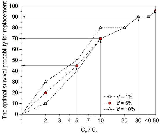
Figure 9.
Influences of on the optimal survival probability for replacement considering different discounted rates.
Table 4 summarizes the influences of model parameters, as well as cost ratios on the optimal corrective and preventive strategies. In general, the model parameter and the ratio are the two most influential factors on the decision-making of maintenance and replacement of water mains.

Table 4.
Summary of effects of model parameters and cost ratios on determination of the optimal and value.
5. Case Study
This section presents the analysis of optimal maintenance and replacement strategies for water mains using model parameters obtained from a real project in a relatively young municipality in Canada. The water mains in the municipality are mainly ductile iron pipes and concrete pressure pipes. This case study focuses on ductile pipes. Most of the pipes were put into service before 1998; the oldest one was installed in 1967. The pipes are typically 400 mm in diameter, and less than 200 m in length. Other information relating to deterioration include pressure zone, surface type, and soil types; however, these pieces of information are not complete. The break records for these pipes are available only after January 1st, 1998. The records are basically the time instances when the breaks took place.
Based on the water main inventory and break records, Lin and Yuan [34] reported that the degradation of ductile iron water mains in the municipality can be modelled by a TTS intensity function including the length and diameter, expressed as:
where and are length and diameter of a water main, respectively; m and mm are constants used to normalize and , respectively. The model parameters were reported to be , , , , and .
Based on the lengths and diameters reported for the municipality by Lin and Yuan [34], we consider an example water main with m and mm. Figure 10 shows the distributions of predictions for the first five breaks for this example water main. The means, medians, and COVs of these predictions are summarized in Table 5. The predictions spread widely, with a COV of 1.055 for the first one, but reducing to 0.546 for the fifth one. The means are 103.0, 148.5, 185.3, 217.0, and 241.4 years. The medians are 64.4, 118.0, 154.9, 194.6, and 218.1 years. Obviously, the distributions of the predictions are not symmetric, since the means and medians are significantly deviated from each other; this deviation reduces for later breaks.
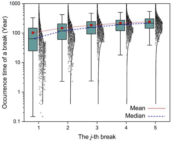
Figure 10.
Predictions of occurrence times for the first five breaks for the example water main.

Table 5.
Mean, median, and COV of predictions of the first five breaks for the example water main.
When corrective strategy is implemented for this water main, it is found that for most cases, the optimal value is under 5. A typical value of 2 or 3 is obtained. This can be expected, as the breaking times are so large (over 100 years) that the gaps of costs due to maintenance or replacement are small in terms of net present value. Similar to earlier analyses, an increase of or a decrease of would lead to a smaller optimal value, as shown in Figure 11.
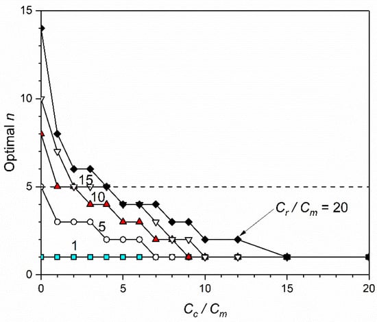
Figure 11.
Influences of and on optimal n value for the example water main.
When a preventive strategy is preferred, the optimal survival probability to carry out a replacement would be 10% for (See Figure 12). If the consequence of failure is much more severe than a replacement, for example, , then the water main is best replaced at a survival probability as early as 40% (or equivalently, the probability of failure reaches 60%). In general, it appears that the best time to implement a replacement of a water main is when its survival probability lies below 50%.
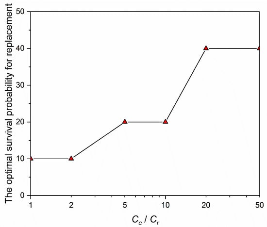
Figure 12.
Influences of on the optimal survival probability for replacement for the example water main.
It is worth mentioning that the model parameters and ratios are firmly based on the case study used here. Though the analysis process can be applied to other cases, caution should be practiced to see whether the values of the parameters and ratios are applicable to those cases or not. It is also worth emphasizing here that the hydraulic pressure at which a water main operates is an important factor for pipe ageing, and thus, for life cycle costing analysis. This factor is not explicitly accounted for in this case study due to the lack of data. Nevertheless, it should be formulated into the intensity function whenever possible to enable a more accurate LCC analysis.
6. Conclusions
This paper presented analyses of both corrective and preventive repair and replacement strategies for water mains. The recurrent water main breaks with increasing service age were modelled as a two-time-scale (TTS) stochastic point process. The corrective strategy was simplified as finding the optimal -th break at which implementing a replacement is more cost-effective than a minimal repair. The preventive strategy is set as determining the optimal survival probability for a water main to receive a replacement. Both strategies were investigated from the perspective of life cycle cost (LCC). The Monte Carlo simulation technique was adopted to conduct the analyses. A case study was illustrated to demonstrate the application of the strategies for real water pipes. The main conclusions drawn from this study are the following.
- (1)
- Both of the optimal corrective and preventive strategies, optimal and , depend highly on the degradation intensity of water mains, as well as the ratios of maintenance, replacement, and failure consequence costs. For corrective strategy, the higher the breaking intensity, the higher the failure consequence loss, and the lower the replacement cost, the lower the optimal value. For preventive strategy, the higher the ratio of consequence loss to replacement cost, the higher the optimal . In addition, the effect of discounting rate diminishes when the ratio of consequence loss to replacement cost becomes large.
- (2)
- The optimal maintenance and replacement strategies are sensitive to the overall shape parameter of the service age in the TTS intensity function, whereas the effects of the scale parameter and the local shape parameter of the sojourn time since the last break on the optimal and are comparatively secondary.
- (3)
- A case study using a typical pipe diameter of 400 mm and length of 200 m shows that the optimal value is typically under 5, and the optimal lies below 50%.
Though the approach adopted in this study for carrying out a life cycle cost (LCC) analysis is easy to implement, it has three limitations. First, the TTS deterioration model is used, which is advantageous, as it takes breaking history into account; however, the parameter estimation for the TTS model would be very computationally demanding if the early break history is missing. Moreover, only the mean of LCC is set as the single target for optimization in this study. If the COV is also considered, then the optimization outcomes could be different. Last, the LCC analysis presented in this study is on individual pipe level, rather than pipe network level. Note that the latter two issues exist not only for this study, but also for many other studies in the literature. It is suggested that the extension from pipe to network level LCC analysis based on the TTS model should be carried out considering multiple objective optimizations. Related topics can be referenced to, e.g., [6,52].
Author Contributions
Conceptualization, P.L., S.H. and B.M.; methodology, P.L.; validation, X.C. and S.H.; formal analysis, X.C.; investigation, P.L.; writing—original draft preparation, P.L.; writing—review and editing, S.H.; supervision, B.M.; funding acquisition, P.L. All authors have read and agreed to the published version of the manuscript.
Funding
This research was funded by the Fundamental Research Funds for the Central Universities, Sun Yat-sen University [22hytd06], the National Natural Science Foundation of China [52008408], the Guangdong Basic and Applied Basic Research Foundation [2021A1515012088], Science and Technology Program of Guangzhou, China [202102021017]. And The APC was funded by the Central Universities, Sun Yat-sen University [22hytd06].
Institutional Review Board Statement
Not applicable.
Informed Consent Statement
Not applicable.
Data Availability Statement
Not applicable.
Conflicts of Interest
The authors declare no conflict of interest.
References
- Sköld, N.-P.; Bergion, V.; Lindhe, A.; Keucken, A.; Rosén, L. Risk-Based Evaluation of Improvements in Drinking Water Treatment Using Cost-Benefit Analysis. Water 2022, 14, 782. [Google Scholar] [CrossRef]
- Liu, Z.; Kleiner, Y.; Rajani, B.; Wang, L.; Condit, W. Condition Assessment Technologies for Water Transmission and Distribution Systems; United States Environmental Protection Agency (EPA): Washington, DC, USA, 2012; EPA/600/R-12/017; p. 108. [Google Scholar]
- Bergion, V.; Lindhe, A.; Sokolova, E.; Rosén, L. Accounting for Unexpected Risk Events in Drinking Water Systems. Expo. Health 2021, 13, 15–31. [Google Scholar] [CrossRef]
- Sjöstrand, K.; Klingberg, J.; Zadeh, N.; Haraldsson, M.; Rosén, L.; Lindhe, A. The Value of Water—Estimating Water-Disruption Impacts on Businesses. Water 2021, 13, 1565. [Google Scholar] [CrossRef]
- Sjöstrand, K.; Lindhe, A.; Söderqvist, T.; Rosén, L. Water Supply Delivery Failures—A Scenario-Based Approach to Assess Economic Losses and Risk Reduction Options. Water 2020, 12, 1746. [Google Scholar] [CrossRef]
- Scholten, L.; Scheidegger, A.; Reichert, P.; Mauer, M.; Lienert, J. Strategic rehabilitation planning of piped water networks using multi-criteria decision analysis. Water Res. 2014, 49, 124–143. [Google Scholar] [CrossRef] [PubMed]
- Sjöstrand, K.; Lindhe, A.; Söderqvist, T.; Rosén, L. Sustainability assessments of regional water supply interventions—Com-bining cost-benefit and multi-criteria decision analyses. J. Environ. Manag. 2018, 225, 313–324. [Google Scholar] [CrossRef]
- van Noortwijk, J.M. Explicit formulas for the variance of discounted life-cycle cost. Reliab. Eng. Syst. Saf. 2003, 80, 185–195. [Google Scholar] [CrossRef]
- van Noortwijk, J.M.; Frangopol, D.M. Two probabilistic life-cycle maintenance models for deteriorating civil infrastructures. Probabilistic Eng. Mech. 2003, 19, 345–359. [Google Scholar] [CrossRef]
- Jardine, A.K.; Tsang, A.H. Maintenance, Replacement, and Reliability: Theory and Applications; CRC Press: Boca Raton, FL, USA, 2005. [Google Scholar]
- Bull, J.W. Life Cycle Costing for the Analysis, Management and Maintenance of Civil Engineering Infrastructure; Whittles Publishing: Dunbeath, UK, 2015. [Google Scholar]
- Campbell, J.D.; Jardine, A.K.; McGlynn, J. Asset Management Excellence: Optimizing Equipment Life-Cycle Decisions; CRC Press: Boca Raton, FL, USA, 2016. [Google Scholar]
- Constantine, A.; Darroch, J. Pipeline Reliability. Stochastic Models in Engineering Technology & Management; Osaki, S., Murthy, D.N.P., Eds.; World Scientific Publishing: Singapore, 1993. [Google Scholar]
- Constantine, G.; Darroch, J.; Miller, R. Predicting underground pipeline failure. Water-Melb. Artarmon. 1996, 23, 9–10. [Google Scholar]
- Economou, T.; Kapelan, Z.; Bailey, T.C. On the prediction of underground water pipe failures: Zero inflation and pipe-specific effects. J. Hydroinform. 2012, 14, 872–883. [Google Scholar] [CrossRef][Green Version]
- Kleiner, Y.; Rajani, B. Using limited data to assess future needs. J. Am. Water Work. Assoc. 1999, 91, 47–61. [Google Scholar] [CrossRef]
- Kleiner, Y.; Rajani, B. I-WARP: Individual Water mAin Renewal Planner. Drink. Water Eng. Sci. 2010, 3, 71–77. [Google Scholar] [CrossRef]
- Le Gat, Y. Extending the Yule process to model recurrent pipe failures in water supply networks. Urban Water J. 2014, 11, 617–630. [Google Scholar] [CrossRef]
- Røstum, J. Statistical Modelling of Pipe Failures in Water Networks. Ph.D. Thesis, Norwegian University of Science and Technology, Trondheim, Norway, February 2000. [Google Scholar]
- Watson, T.G.; Christian, C.D.; Mason, A.J.; Smith, M.H.; Meyer, R. Bayesian-based pipe failure model. J. Hydroinform. 2004, 6, 259–264. [Google Scholar] [CrossRef][Green Version]
- Mailhot, A.; Pelletier, G.; Noël, J.-F.; Villeneuve, J.-P. Modeling the evolution of the structural state of water pipe networks with brief recorded pipe break histories: Methodology and application. Water Resour. Res. 2000, 36, 3053–3062. [Google Scholar] [CrossRef]
- Pelletier, G.; Mailhot, A.; Villeneuve, J.-P. Modeling water pipe breaks—Three case studies. J. Water Resour. Plan. Manag. 2003, 129, 115–123. [Google Scholar] [CrossRef]
- Scheidegger, A.; Scholten, L.; Maurer, M.; Reichert, P. Extension of pipe failure models to consider the absence of data from replaced pipes. Water Res. 2013, 47, 3696–3705. [Google Scholar] [CrossRef]
- Clair, A.M.S.; Sinha, S. State-of-the-technology review on water pipe condition, deterioration and failure rate prediction models. Urban Water J. 2012, 9, 85–112. [Google Scholar] [CrossRef]
- Kleiner, Y.; Rajani, B. Comprehensive review of structural deterioration of water mains: Statistical models. Urban Water 2001, 3, 131–150. [Google Scholar] [CrossRef]
- Nishiyama, M.; Filion, Y. Review of statistical water main break prediction models. Can. J. Civ. Eng. 2013, 40, 972–979. [Google Scholar] [CrossRef]
- Rajani, B.; Kleiner, Y. Comprehensive review of structural deterioration of water mains: Physically based models. Urban Water 2001, 3, 151–164. [Google Scholar] [CrossRef]
- Scheidegger, A.; Leitão, J.P.; Scholten, L. Statistical failure models for water distribution pipes—A review from a unified perspective. Water Res. 2015, 83, 237–247. [Google Scholar] [CrossRef] [PubMed]
- Termes-Rifé, M.; Molinos-Senante, M.; Hernández-Sancho, F.; Sala-Garrido, R. Life Cycle Costing: A tool to manage the urban water cycle. J. Water Supply Res. Technol. 2013, 62, 468–476. [Google Scholar] [CrossRef]
- Roshani, E.; Filion, Y.R. Event-Based Approach to Optimize the Timing of Water Main Rehabilitation with Asset Management Strategies. J. Water Resour. Plan. Manag. 2014, 140, 04014004. [Google Scholar] [CrossRef]
- Naoum-Sawaya, J.; Ghaddar, B.; Arandia, E.; Eck, B. Simulation-optimization approaches for water pump scheduling and pipe replacement problems. Eur. J. Oper. Res. 2015, 246, 293–306. [Google Scholar] [CrossRef]
- Lee, H.; Shin, H.; Rasheed, U.; Kong, M. Establishment of an Inventory for the Life Cycle Cost (LCC) Analysis of a Water Supply System. Water 2017, 9, 592. [Google Scholar] [CrossRef]
- Ghobadi, F.; Jeong, G.; Kang, D. Water Pipe Replacement Scheduling Based on Life Cycle Cost Assessment and Optimization Algorithm. Water 2021, 13, 605. [Google Scholar] [CrossRef]
- Lin, P.; Yuan, X.-X. A two-time-scale point process model of water main breaks for infrastructure asset management. Water Res. 2018, 150, 296–309. [Google Scholar] [CrossRef]
- Lin, P.Y.; Yuan, X.X.; Tovilla, E. Integrative modeling of performance deterioration and maintenance effectiveness for infrastructure assets with missing condition data. Comput. Aided Civ. Infrastruct. Eng. 2019, 34, 677–695. [Google Scholar] [CrossRef]
- Yuan, X.X. Principles and guidelines of deterioration modelling for water and waste water assets. Infrastruct. Asset. Manag. 2017, 4, 19–35. [Google Scholar] [CrossRef]
- Cox, D.R.; Isham, V. Point Processes; Taylor & Francis: Abingdon, UK, 1980. [Google Scholar]
- Cook, R.J.; Lawless, J.F. The Statistical Analysis of Recurrent Events; Springer: Berlin/Heidelberg, Germany, 2007. [Google Scholar] [CrossRef]
- Jacobsen, M. Point Process Theory and Applications: Marked Point and Piecewise Deterministic Processes; Springer Science & Business Media: Berlin/Heidelberg, Germany, 2006. [Google Scholar]
- Daley, D.J.; Vere-Jones, D. An Introduction to the Theory of Point Processes: Volume II: General Theory and Structure; Springer: New York, NY, USA, 2007. [Google Scholar]
- Lin, P.; Yuan, X.-X. An Advanced Statistical Method for Point Process Modelling with Missing Event Histories. IEEE Access 2020, 8, 210081–210098. [Google Scholar] [CrossRef]
- Pietrucha-Urbanik, K. Failure Prediction in Water Supply System—Current Issues; Springer: Berlin/Heidelberg, Germany, 2015; pp. 351–358. [Google Scholar] [CrossRef]
- Pietrucha-Urbanik, K. Assessing the Costs of Losses Incurred as a Result of Failure; Springer: Berlin/Heidelberg, Germany, 2016; pp. 355–362. [Google Scholar] [CrossRef]
- Pietrucha-Urbanik, K.; Tchórzewska-Cieślak, B. Cost Analysis of Water Pipe Failure; Springer: Berlin/Heidelberg, Germany, 2020; pp. 411–424. [Google Scholar]
- Hashemi, B.; Najafi, M.; Mohamed, R. Cost of Underground Infrastructure Renewal: A Comparison of Open-Cut and Trenchless Methods. In Proceedings of the 12th International Pipelines Conference 2008, Atlanta, GA, USA, 22–27 July 2008. [Google Scholar]
- Najafi, M.; Gokhale, S.B. Trenchless Technology: Pipeline and Utility Design, Construction, and Renewal; McGraw-Hill Education: New York, NY, USA, 2005. [Google Scholar]
- Wu, Y.; Kang, C.; Nojumi, M.M.; Bayat, A.; Bontus, G. Current water main rehabilitation practice using trenchless technology. Water Pract. Technol. 2021, 16, 707–723. [Google Scholar] [CrossRef]
- Yang, M.-D.; Su, T.-C.; Wu, T.-Y.; Huang, K.-S. No-Dig Inspection Technologies for Underground Pipelines. J. GeoEng. 2010, 5, 99–104. [Google Scholar]
- Zhao, Y.; Ma, B.; Ariaratnam, S.T.; Zeng, C.; Yan, X.; Wang, F.; Wang, T.; Zhu, Z.; He, C.; Shi, G.; et al. Structural performance of damaged rigid pipe rehabilitated by centrifugal spray on mortar liner. Tunn. Undergr. Space Technol. 2021, 116, 104117. [Google Scholar] [CrossRef]
- Lemer, A. Life Cycle Costing: For the Analysis, Management and Maintenance of Civil Engineering Infrastructure. Constr. Manag. Econ. 2015, 33, 689–691. [Google Scholar] [CrossRef]
- van den Boomen, M.; Schoenmaker, R.; Wolfert, A.R.M. A life cycle costing approach for discounting in age and interval replacement optimisation models for civil infrastructure assets. Struct. Infrastruct. E 2018, 14, 1–13. [Google Scholar] [CrossRef]
- Mittal, A.; Scholten, L.; Kapelan, Z. A review of serious games for urban water management decisions: Current gaps and future research directions. Water Res. 2022, 215, 118217. [Google Scholar] [CrossRef]
Publisher’s Note: MDPI stays neutral with regard to jurisdictional claims in published maps and institutional affiliations. |
© 2022 by the authors. Licensee MDPI, Basel, Switzerland. This article is an open access article distributed under the terms and conditions of the Creative Commons Attribution (CC BY) license (https://creativecommons.org/licenses/by/4.0/).