Article

The Effect of Spatial Input Data Quality on the Performance of the SWAT Model

1
Institute of Ecology and Earth Sciences, University of Tartu, Vanemuise 46, 51014 Tartu, Estonia
2
Department of Civil Engineering, Indian Institute of Technology-Madras, Chennai 600036, India
*
Author to whom correspondence should be addressed.
Water 2022, 14(13), 1988; https://doi.org/10.3390/w14131988
Submission received: 3 May 2022 / Revised: 29 May 2022 / Accepted: 17 June 2022 / Published: 21 June 2022
(This article belongs to the Special Issue Advances and Challenges in Hydrological Modeling and Engineering)

Abstract

:
Soil and land use information are important inputs for physically-based hydrological modeling such as SWAT. Although fine resolution local or regional data are often preferred for modeling, it is not always reliable that these data can lead to better model performance. In this study, we investigate the effect of input data on the sensitivity and uncertainty of the SWAT model in the Porijõgi catchment in Estonia. We created four model setups using global/regional level data (HWSD soil and CORINE) and local high-resolution spatial data, including the Estonian high-resolution EstSoil-EH soil dataset and the Estonian Topographic Database (ETAK). We employed statistical criteria to assess SWAT model performance for monthly simulated stream flows from 2007 to 2019. The results illustrated that models with high-resolution local soil data performed lower than models with global soil data, but in contrast, in the case of land use datasets, the local high-resolution ETAK dataset improved performance over the CORINE data.

1. Introduction

Hydrological systems are often complicated due to high temporal variability and diverse topography, land use, and anthropogenic conditions in the catchments. Hydrological models have become indispensable for understanding these complex human–ecosystem interactions and investigating the effects of human activities on watershed systems [1]. Over the past few decades, intensive efforts have been made to develop process-based catchment models operating on different temporal and spatial scales. Such models include, for example, Topographic Hydrological Model (TOPMODEL) [2], Système Hydrologique Européen (MIKE-SHE) [3], and the Soil and Water Assessment Tool (SWAT) [4]. Various process-based models have been extensively applied worldwide to improve the understanding of hydrological processes and provide scientifically credible solutions. However, SWAT has gained wide popularity and was chosen in this study due to its open-access nature, compatibility with geospatial tools, spatial and temporal flexibility, and incorporation of optimization algorithms [1,5].
SWAT requires detailed information on soil, land use, topography, and weather to successfully set up, execute and interpret the results [6]. Such spatial datasets need to be high quality and reliable to produce trustworthy model responses. However, many specific data requirements such as soil hydraulic conductivity or soil bulk density cannot be measured everywhere and, thus, are modeled or derived in other ways to create spatial coverage for these parameters. Consequently, these types of data are often exposed to various levels of errors associated with data sources, resolution, interpolation, and resampling techniques [6,7]. Such errors combined with an inaccurate model structure can lead to uncertainties in the modeling outputs [8,9]. Model uncertainty analysis plays a key role in identifying the magnitude and sources of errors and enables more adequate decision-making [8,10]. Failure to understand and interpret the effects of these uncertainties on model performance may result in model outputs that cannot consistently represent the observations.
In recent years, the sensitivity of the SWAT model to spatial input data has attracted the attention of researchers [6,8,11,12,13]. The previous studies show somewhat contradicting results, and there is no clear pattern indicating that high-resolution and local data outperform the low-resolution data. For example, Camargos et al. [6] evaluated the effect of spatial resolution of the input data on river discharge simulation and found that regional land use data reduced the bias of discharge simulation by 50%, while global soil data performed better than regional soil. On the contrary, Geza and McCray [14] evaluated the performance of SWAT with two U.S. soils (i.e., high-resolution SSURGO and low-resolution STATSGO soils) and reported better performance of the model with SSURGO soil. Al-Khafaji et al. [12] investigated the effect of DEM and land use data quality on the accuracy of SWAT model predictions and reported that high-resolution datasets did not provide better predictive reliability. Similar results were obtained by Asante et al. [11], who evaluated the impact of land use data quality on the predictive capacity SWAT model and indicated slightly better performance of low-resolution land use data. Chaplot [15] also confirmed only a little impact of land use quality on the SWAT model results, while soil data with lower resolution greatly degraded the prediction accuracy. In general, the existing studies on the effect of spatial input data resolution (especially soil and land use) on SWAT estimates have yielded contradicting conclusions. Such contradictions mainly arise from the variations in environmental characteristics of the investigated watersheds [15]. As a result, it is essential to evaluate the sensitivity of the SWAT model to the accuracy of these datasets in catchments differing in physiographic conditions.
Moreover, previous studies have focused on evaluating the effect of input data uncertainty on SWAT model predictions using low-resolution global or regional datasets, while no attention has been given to assessing the effect of high-resolution local datasets. In this paper, we examined the effect of high-resolution local soil and land use data on the predictive capacity of the SWAT model in the Porijõgi catchment of Estonia. We hypothesized that local datasets provide greater information details and yield a reduced range of parameter uncertainty and better simulation performance than global or regional lower-resolution datasets.

2. Materials and Methods

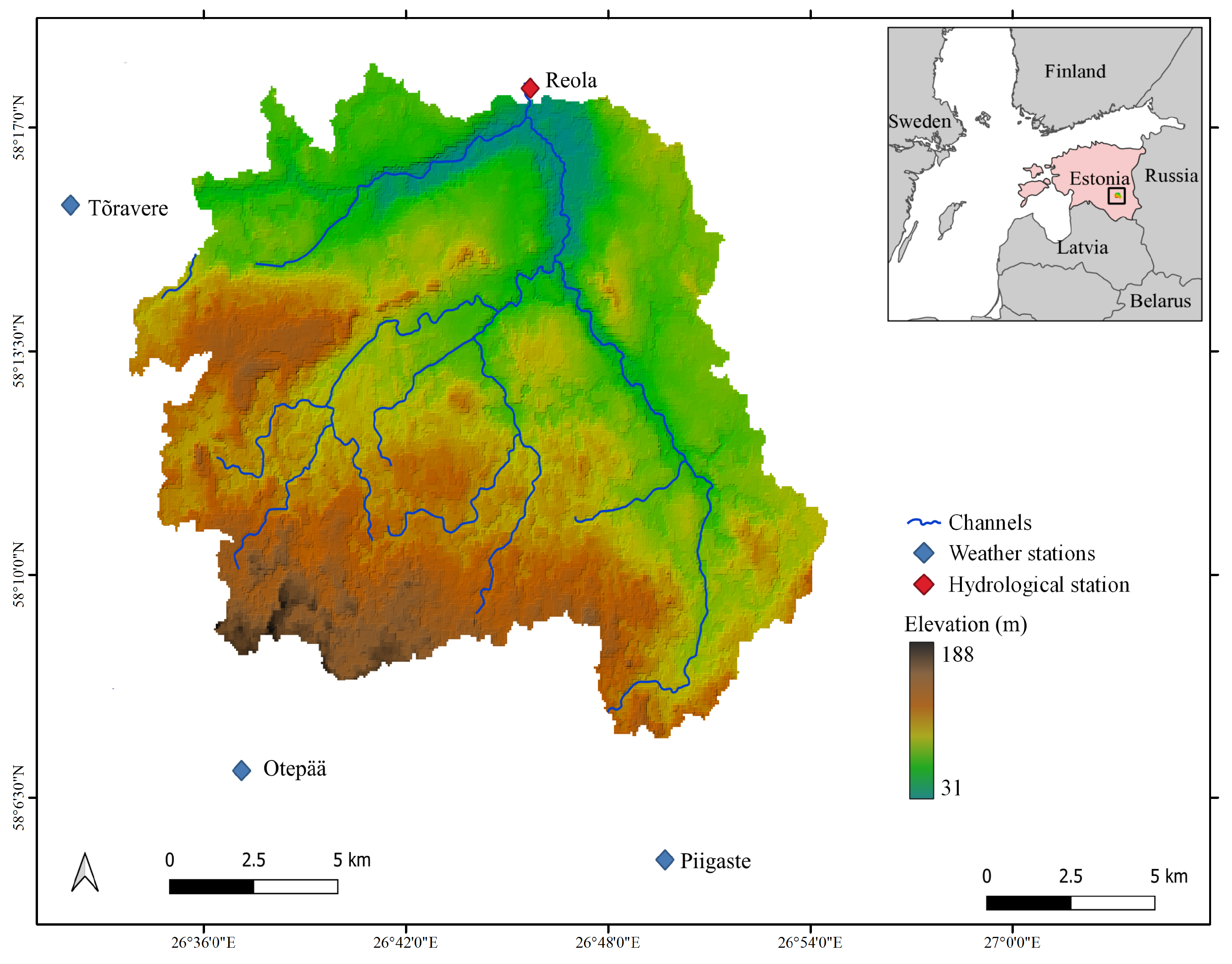
2.1. Description of the Study Area
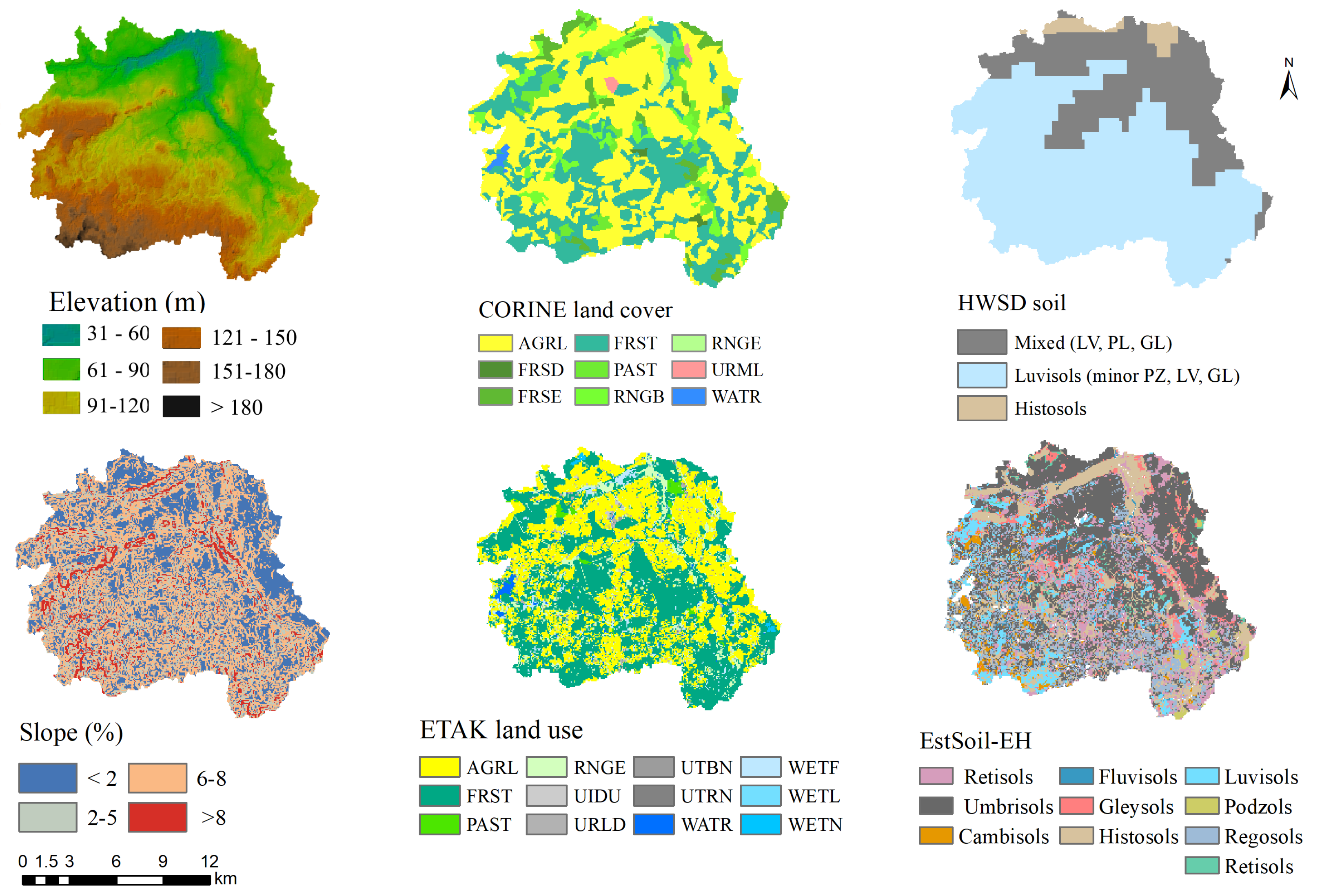
The Porijõgi catchment, with a total area of 258 km 2 , is one of the Emajõgi river sub-catchments in Estonia (Figure 1). The central and northern part of the catchment is in the southern Estonian moraine plain, 5–10 km south of Tartu city. The catchment elevation varies between 31 and 188 m above mean sea level (a.s.l). A major part of the catchment is located on the Otepää Heights with a fragmented landscape [16]. The depth of the groundwater table varies (0.5–20 m) depending on relief and geomorphologic conditions [17]. The northern part of the catchment is covered by patches of fields, grasslands, and forests, while the southern part is a very mosaic landscape [18]. Upland areas of the catchment are dominated by podzoluvisols, planosols, and podzols on loamy sand and fine sandy loam [19]. The main crops grown in the catchment include wheat and rapeseed, with mainly mineral fertilizers used [20]). The average annual precipitation during the research period (2007–2019) is 678 mm, and the mean annual temperature is 6.38 °C [13].

2.2. Input Data

We used MERIT DEM [21] for elevation data (70 m resolution) to derive the catchment. For soil and land use data, we used both high-resolution local and lower-resolution regional and global level information (Figure 2). For global soil data, we used the Harmonized World Soil Database (HWSD 2.1), which has a 1 km spatial resolution [22]. For local soil data, we used EstSoil-EH [23], which is 1:10,000 scale vector data with 75% of mapped units smaller than 4.0 ha. Each mapped unit has a unique composition of soil parameters, including depth of profile and horizons, texture, and fine earth fractions, etc. To represent this highly detailed and spatially varying data in a useful way to SWAT, we converted it to raster with a resolution of ca. 70 m, which is the same resolution as the MERIT DEM used for catchment delineation. The CORINE Land Cover data (100 m) for the year 2012 was used as regional/global lower-resolution land use data, which has a defined minimum mapping unit of 25 ha [24]. For the local land use data, we used Estonian Topographic Database (ETAK) (1:10,000) obtained from the Estonian Land Board [25]. The local land use is more detailed than CORINE, especially in urban land use and wetlands spatial distribution. In CORINE, the generic-agricultural land (ca. 50%) dominates the catchment, followed by mixed forests (32.3%). In ETAK land use, on the other hand, the mixed forest (45.8%) dominates the study area, while the share of agricultural land is only 38% (Table 1).
The daily weather records (2007–2019), which included precipitation, maximum and minimum temperature, solar radiation, relative humidity, and wind speed, were collected from the Estonian Weather Service (EWS) database at 3 stations (Tõravere, Piigaste, and Otepää). The daily average streamflow (m 3 /s) of the Porijõgi (2007–2019) was obtained from EWS at the Reola gauge, located at the outlet of the catchment.

2.3. Model Setup

We built four models for the Porijõgi, where we use different soil and land use data combinations while keeping the other inputs constant, such as DEM, subbasins, and hydro-climate forcing data (Table 2). We used the QSWAT3 plugin [26] to set up the models. The catchment delineation and overlay of spatial datasets were performed automatically within the interface. We used the threshold of 3.6 km 2 to divide the catchment into 37 subbasins, which was kept the same in all models. QSWAT further subdivided the subbasins into different hydrological response units (HRUs). The interface discretizes unique combinations of soil type, land cover, and slope classes within each sub-basin into several HRUs based on a defined threshold. Reference [6] suggested not using any threshold to avoid loss of both information and representation of heterogeneity, and in their case study area of 104 km 2 created 100–200 HRUs at the greatest detail. The number of HRUs varies depending on the distribution and resolution of land use and soil. However, we chose a threshold of 10% of the subbasin area to keep the number of HRUs and, thus, simulation time manageable.
In order to compare the impact on the model performance and to be able to attribute these effects to the different input data (i.e., land use and soil), we implemented the following steps:
  • First, each of the four models is calibrated and validated individually to understand and assess their capability to predict streamflow in the catchment by itself.
  • Secondly, we collate the calibrated parameter ranges from each individual model into an encompassing range for each originally selected parameter. With this parameter configuration, we run a sensitivity analysis for each model.
  • Finally, we reduce the list of parameters from the previous step to only the sensitive parameters and their ranges, run a final uncertainty analysis again, and extract the results.
These steps are described in more detail in Section 2.4Section 2.6.

2.4. Calibration and Validation

For flood forecasting, reservoir management or other operational applications of SWAT, daily streamflow simulation is of importance. For the general characterization and management of a catchment and to understand and describe the hydrological system, monthly flows are an appropriate scale to identify patterns to see the “big picture”. Furthermore, Moges et al. [13] reported high daily variation in the detection of rainfall in the observed gauges for the Porijõgi catchment. Thus, we calibrated and validated all models only on a monthly scale to reduce additional noise.
The initial model calibration and validation were achieved using SUFI-2 in SWAT-Calibration and Uncertainty Program (SWAT-CUP) [27]. We identified the ranges of the parameters based on the SWAT manual [28] and used the one-at-a-time approach. We calibrated the models using 2007 to 2014 and validated them using years from 2015 to 2019 on a monthly time scale. The first two years (2005–2006) were used as a warm-up period to mitigate the unknown initial conditions. Snow-related parameters were calibrated independently from the main parameters, fixed, and excluded from further calibration [29]. Several simulation iterations (500–2000 simulations in each run) were executed until we achieved a reasonable value of statistical metrics. After each iteration, we modified (narrowed down) the range of parameters based on the new parameter ranges suggested by SWAT-CUP. In the validation step, the models were simulated for a separate period not included in the calibration, keeping the same number and range of parameters used for calibration. The performance and efficiency of the models in simulating the observed streamflow were evaluated using the Nash–Sutcliffe Efficiency (NSE) [30] as the goodness-of-fit between observed and simulated streamflow.

2.5. Sensitivity Analysis

The models were initially calibrated and validated independently to assess the combination of input data separately and to describe initial model robustness. After we calibrated and validated the models individually, we re-traced the basic modeling steps jointly across all models. In particular, we applied a global sensitivity analysis in SWAT-CUP to find those parameters that significantly influence the streamflow. We considered the same parameters (Table 3) as at the start of each individual calibration step, but we collated the finalized calibrated parameter ranges from each individual model into an encompassing range for each originally selected parameter into a single parameter file. The global sensitivity analysis considers the sensitivity of the simulated streamflow values to changes in one parameter in relation to the other changed parameters. We used the t-stat for impact and p-value to assess the sensitivity rank of the parameters. Then, we selected those parameters where the p-value was less than the 0.05 level. The parameters with a p-value less than 0.05 in at least one of the four models were chosen as sensitive parameters and used for the subsequent joint parameter-based uncertainty analysis.

2.6. Joint Parameter-Based Evaluation of Differences in Model Performance

We ran an additional uncertainty analysis with the developed single parameter list for all the models and set the simulations for 2000 runs during this last step. We extracted and compared the simulated parameter ranges from this uncertainty analysis simulation with the Python package pyswat [31] for the top 5% performing simulations (the 95% percentile of NSE, not 95PPU) for each of the models. To statistically assess differences or similarities between the parameter value distributions for the models with their different combinations of land use and soil input data, we applied crosswise comparison using the Mann–Whitney-U test [32] and visualized the results as individual heatmaps per parameter.

3. Results

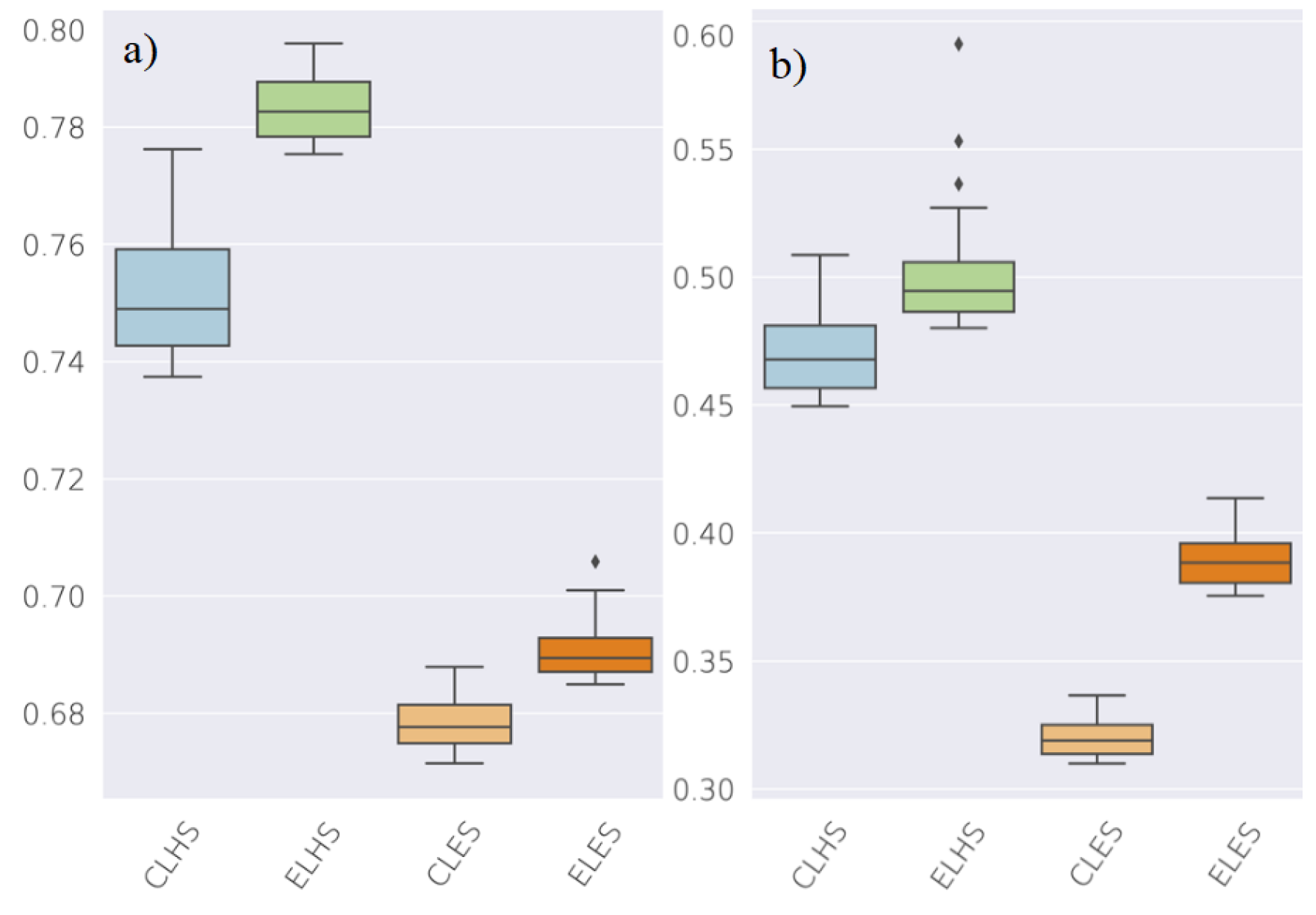
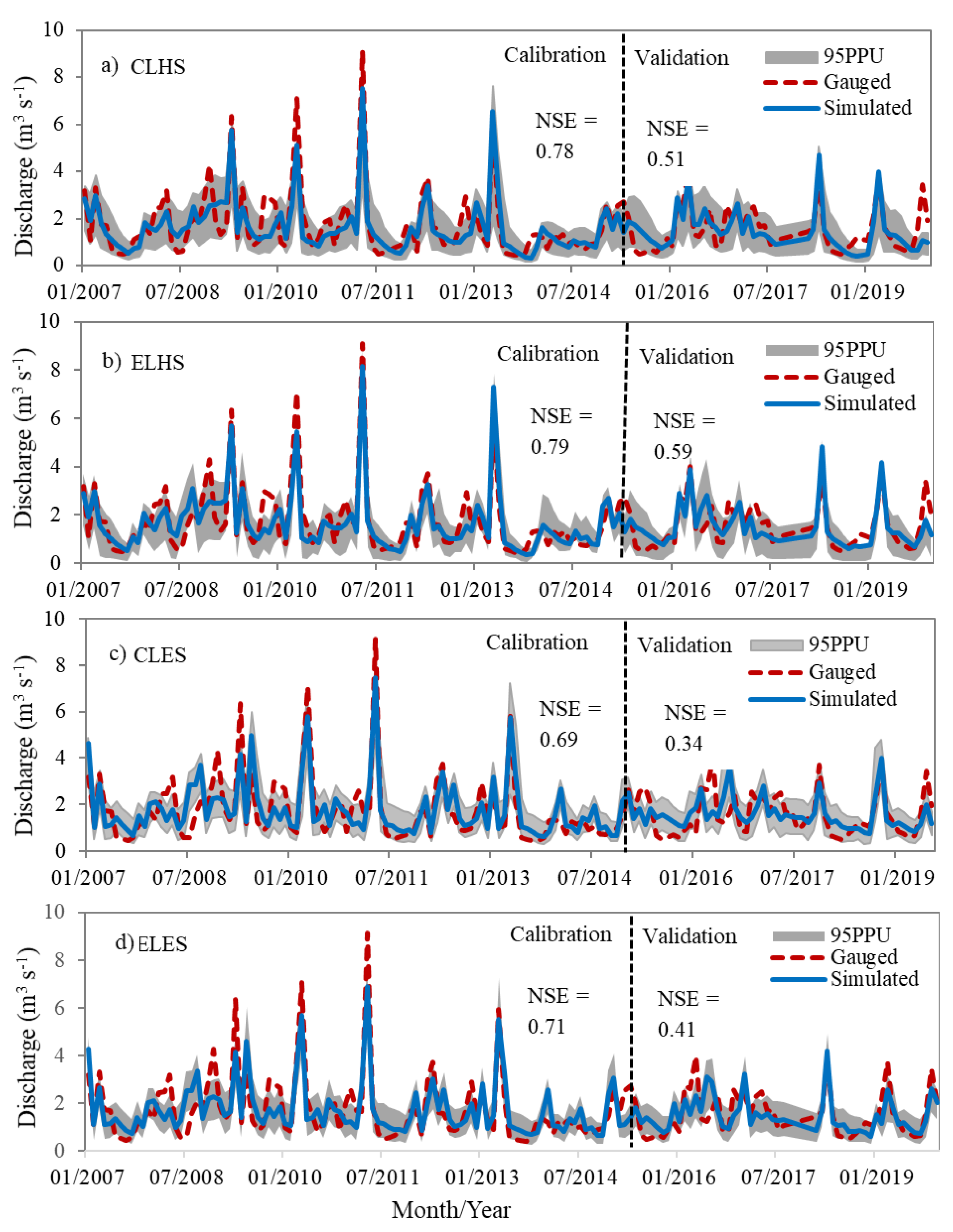
3.1. General Model Performance

All four models achieved a very good performance in predicting streamflow during calibration, but for the validation period, only the models with the global HWSD soil (CLHS and ELHS) achieved good or at least satisfactory performance, but the two models with local EstSoil-EH (CLES and ELES) were below satisfactory level (Table 4). The soil datasets had a strong influence on the model performance, whereas the effect of different land use data was less influential. The models with HWSD soil performed very well, whereas the models with EstSoil-EH did not reach similarly high NSE values. However, among the models with the same soil data, those models with the local Estonian land use data performed better than models with regional CORINE land cover.
The goodness-of-fit between the simulated and the measured discharges was evaluated by using the P-factor (the percentage of data bracketed by the 95% prediction uncertainty band-95PPU) and R-factor (a measure of the thickness of the 95PPU band) indices. Abbaspour [33] recommended a value of >0.7 for the P-factor and <1.5 for the R-factor for discharge simulations. Our results indicate that most of the models fall in the desirable ranges of the two indices (Table 4 and Figure 3). Although CLHS and ELHS models yielded slightly lower values for validation, all models resulted in a P-factor higher than 0.7, suggesting that over 70% of the measured discharges were enveloped by the 95PPU. Similarly, except for the CLES model during validation, all models yielded an R-factor less than 1.5, which indicates that the observed discharge and the 95PPU matched very well. Our results also reveal the PBIAS values of < ± 10 for both calibration and validation periods, indicating a “very good” level of performance for all models [34]. Figure 3 indicates that all models captured the low flow better, while most of the peak flows were underestimated (positive PBIAS).

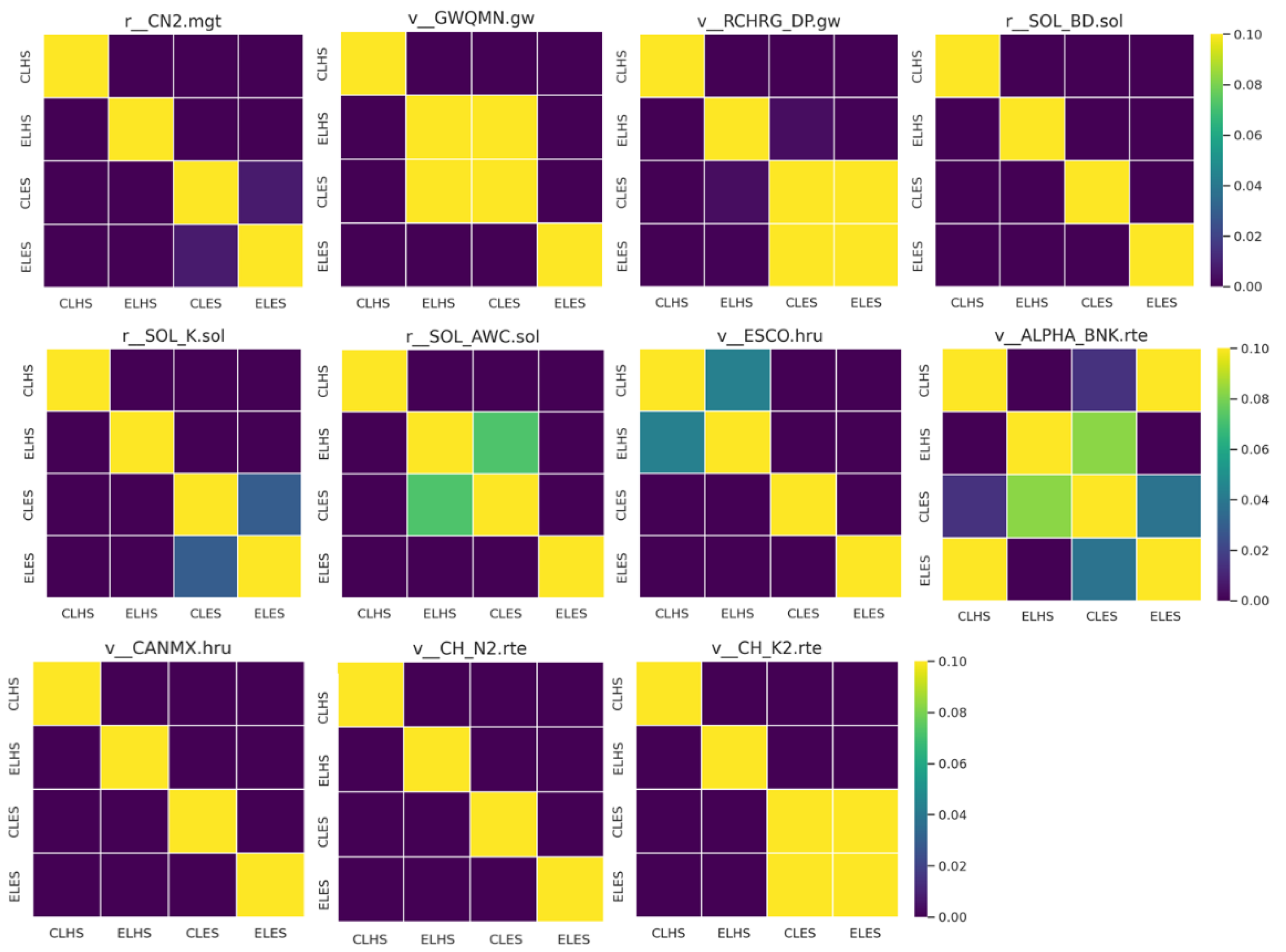
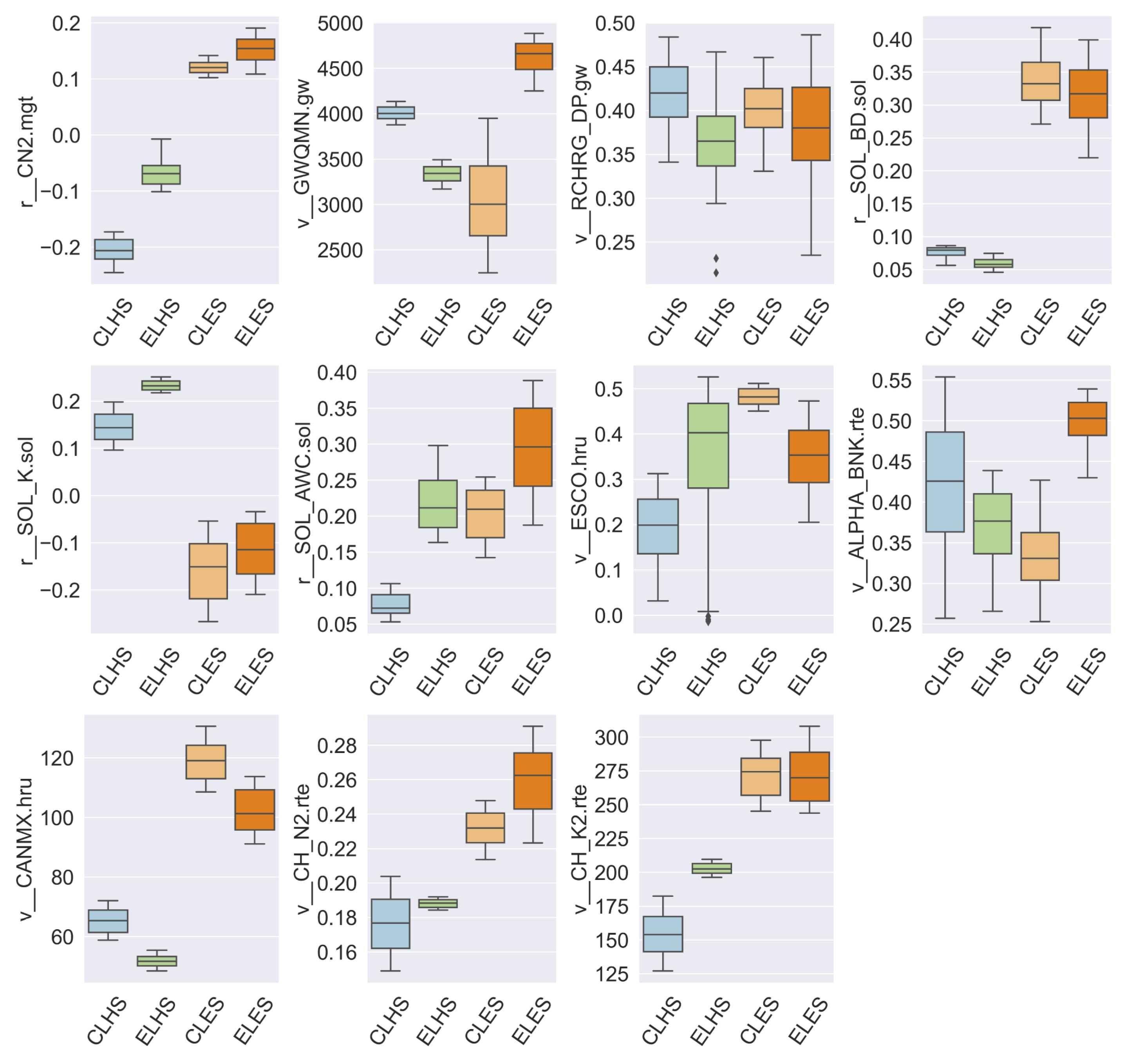
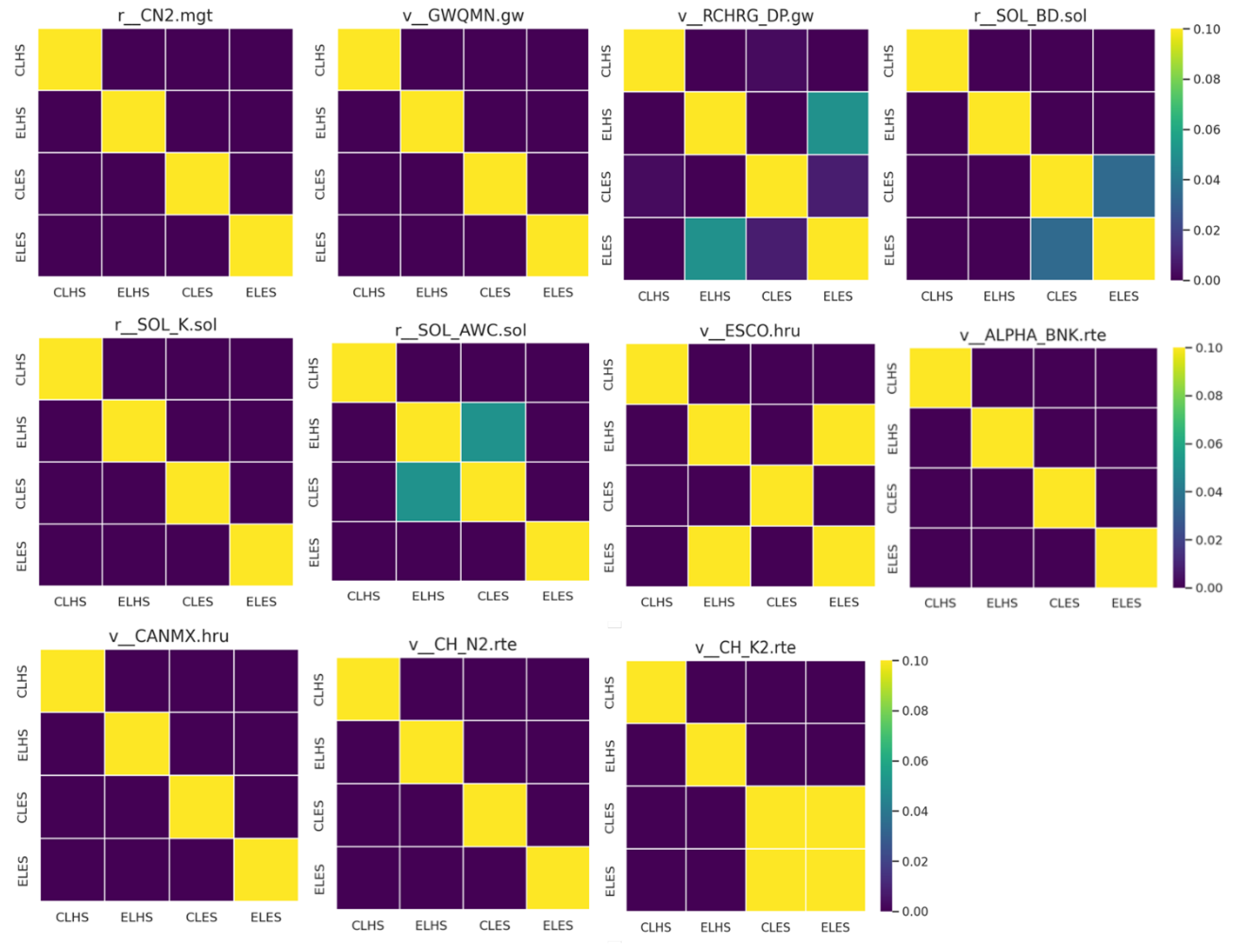
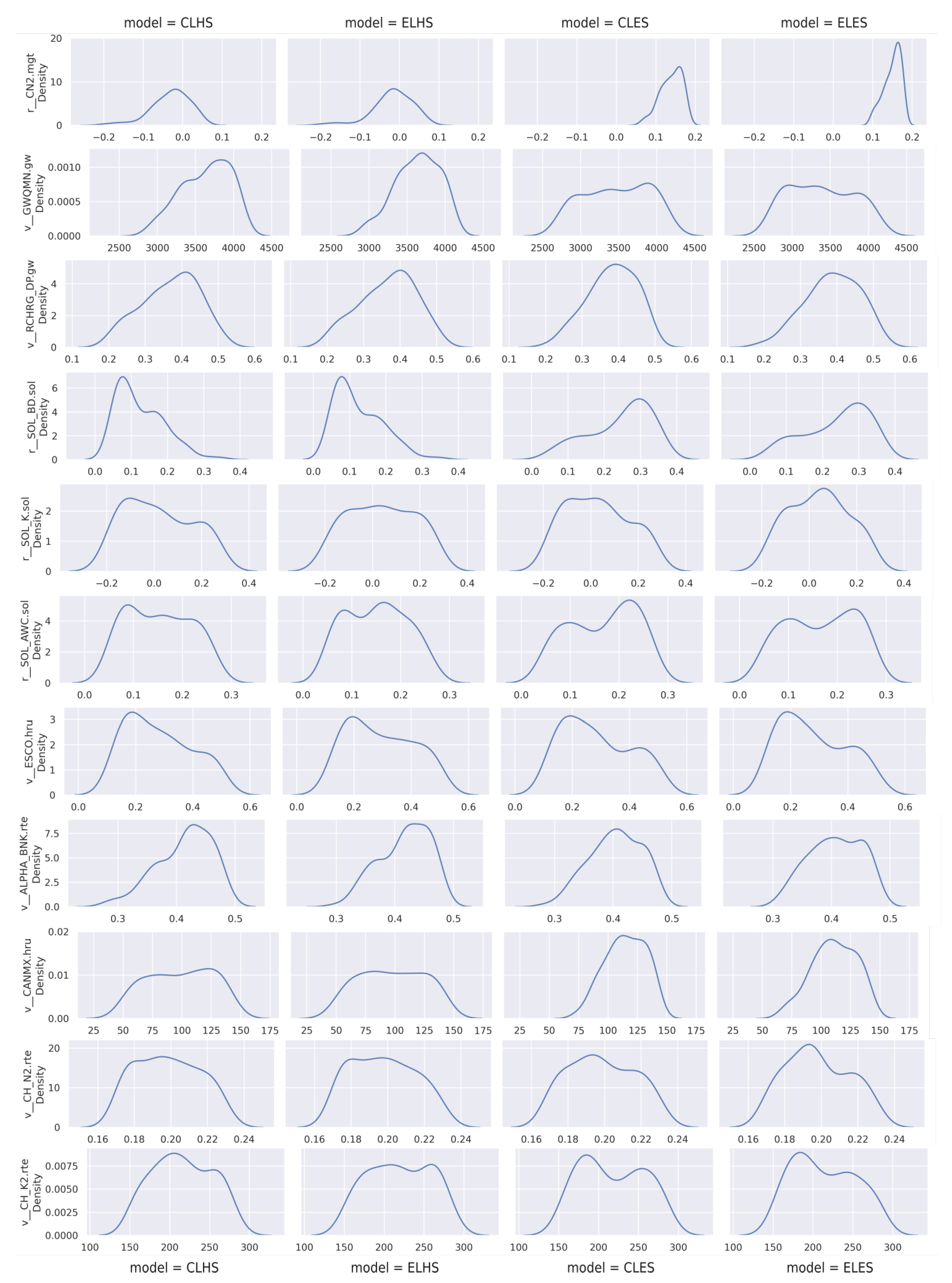
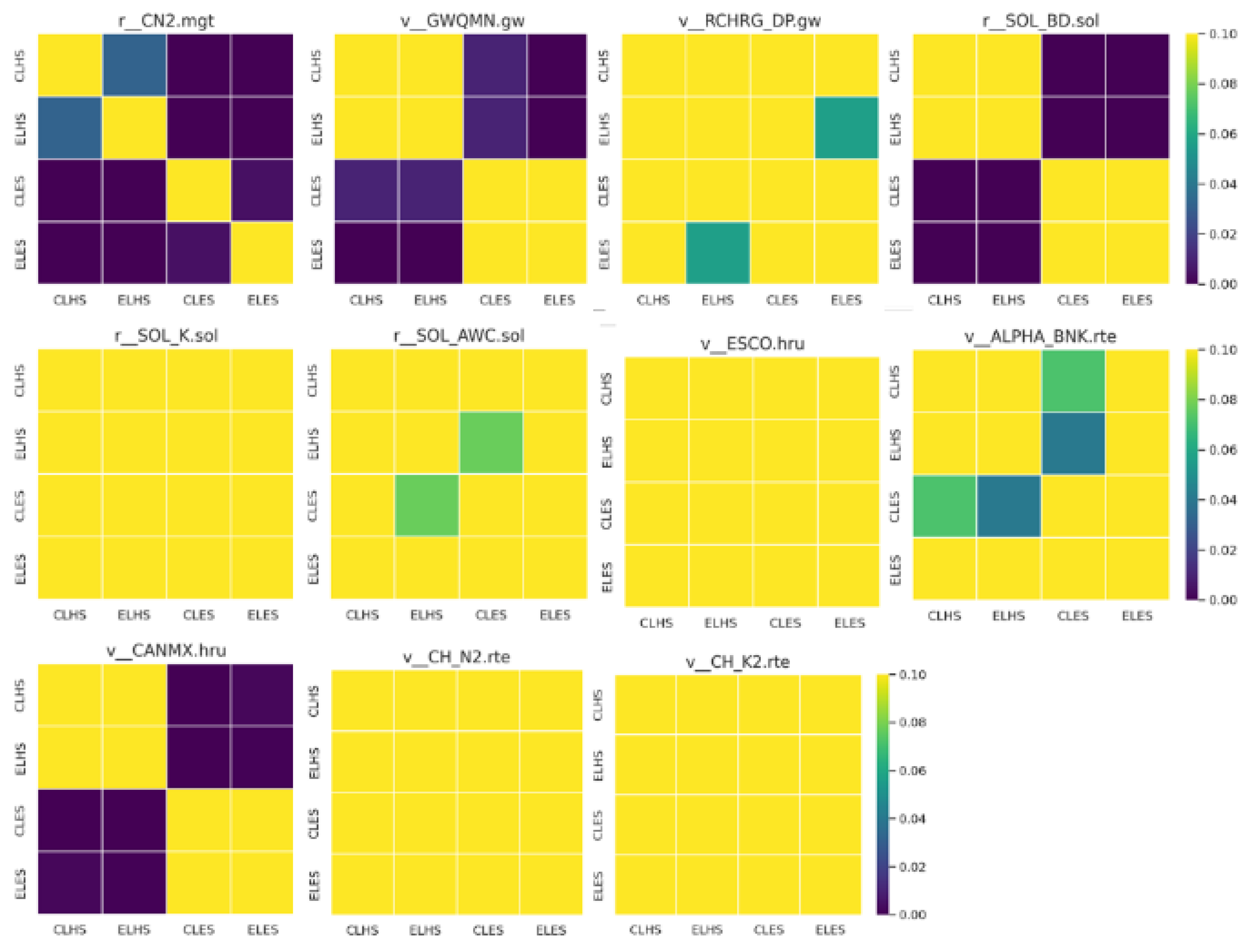
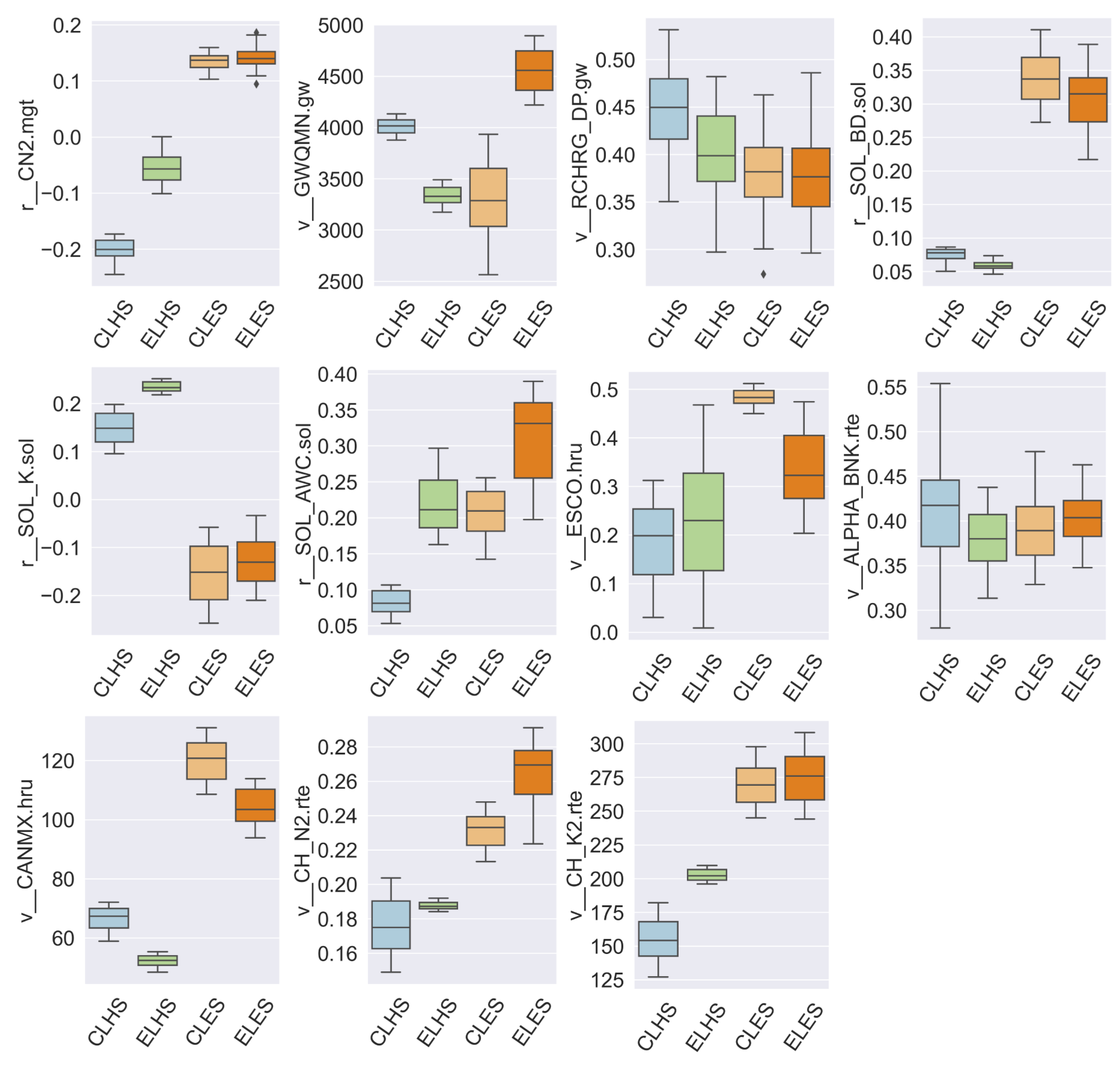
3.2. Joint Parameter Level Performance Assessment

The joint parameter level performance assessment, which is still a traditional parameter uncertainty assessment but with equalized all-encompassing parameter ranges for all four models, followed the individual model assessment. The list of parameters only contains sensitive parameters based on a prior global sensitivity analysis. The same value distributions for the fitted parameters are extracted for the 5% performing simulations.
In Figure 4, it becomes apparent that the preferential parameter ranges for high-performing simulations are much more similar to the models that use the same soil input data. In particular, the similarity of the value distributions for the parameters curve number (CN2), shallow aquifer return flow (GWQMN), bulk density (SOL_BD), and canopy storage (CANMX) is very pronounced (Figure A6 shows the detailed density plot).
The models with EstSoil-EH (ELES and CLES) show a preference for increasing CN2 (Figure A6, row 1), which indicates a strong tendency to increase surface runoff. GWQMN has a more defined peak for the models with HWSD soil (ELHS and CLHS), whereas, for ELES and CLES, the density curve is flatter and indicates a less defined behavior (Figure A6, row 2). SOL_BD exhibits a very significant trend in both cases. For ELHS and CLHS, the simulations optimize only for a small increase, with the density plot showing a positive skew (Figure A6, row 4), but for ELES and CLES, the trend is inverse, with a much stronger tendency and higher values for SOL_BD and negative skew. Finally, CANMX values are optimized for larger canopy storage in the ELES and CLES models (Figure A6, row 9).
We used the Mann–Whitney-U test to compare the extracted parameter values as groups pair-wise per parameter per model. The heatmaps in Figure 5 visualize whether there is a statistically significant difference between the model parameter ranges. Statistical significance (p < 0.05, dark-green to purple) indicates that we can reject the null hypothesis that the two model parameter ranges are similar. Thus, where the squares are dark green-purple, we can say that the parameter ranges of the two models are statistically significantly different. The only meaningful patterns can be reported for CN2 (1) GWQMN (2), SOL_BD (4), and CANMX (9), with a striking clustering based on the soil data of the model (Figure 5, l. to r., from top). Figure A3 and Figure A5 in the appendix show the results of this Mann–Whitney-U analysis for the initial calibration and validation steps for the models. In the calibration, almost all parameter distributions are different from each other, which is rooted in their individual initial calibration and optimizations. Whereas in the validation, we saw only significant differences between models with different soil data sets (Figure 5).
In order to interpret the initial parameterization of the soils based on the input datasets, we compared the general soil textures and fine earth fractions from the discretized HRUs before any calibration. We summarized the parameter values for the significantly differing parameters and additional explanatory variables (SAND, SILT, CLAY, ROCK, and Hydrologic Soil Group) and area- and depth-weighted them accordingly into a per-catchment-model summary table (Table 5).
EstSoil-EH states a much higher sand to silt content ratio: 10–15% more sand in EstSoil-EH versus 10–15% higher silt fractions in HWSD for the Porijõgi catchment. The clay fractions are much more similar. Both data sets HWSD and EstSoil-EH hydrologically emulate wetlands and histosols with a high clay fraction. For EstSoil-EH, we see higher soil organic carbon and lower bulk density values than in HWSD.
Figure A2 and Figure A4 in the appendix show the parameter value distributions of the top 5% performing simulations during the calibration and validation period, and Figure A1 shows the ranges of NSE as boxplots for the extracted simulations. These ranges were already constrained and optimized through each model’s individual calibration iterations and demonstrate the preferential value ranges for each model.

4. Discussion

In this study, we compared low to medium resolution datasets of land use (CORINE) and soil (HWSD) with local high-resolution datasets (ETAK, EstSoil-EH) in a four-fold cross-wise fashion to answer the question of whether local datasets yield a better simulation performance and can reduce parameter uncertainty when predicting streamflow with SWAT. The results indicate a mixed response. The models with the high-resolution local soils performed worse; however, the models with the same soil but with the high-resolution Estonian land use data performed marginally better. Overall, the impact of the soil datasets was stronger on the model uncertainty.
Overall, all models captured the low flow better, while many of the peak flows were underestimated (positive PBIAS), which might be due to the very mosaic nature of the catchment and the abundance of floodplains with alluvial soils in the lower catchment that delay the flow peak. In general, it can be said that the values obtained for the P-factor and R-factor (Table 4) indicate low uncertainties for all individual models. Higher uncertainties can only be observed for validation, which is expected. All models exhibit a decline in NSE values for the validation period within a range of 0.2 to 0.3, with the best model, ELHS (Estonian landuse, HWSD soil), also having the best scores during validation (cf. Figure 3). This could indicate over-fitting during calibration. One reason for the lower validation scores could be that the three rain gauges are not fully capturing the variability of the rainfall within the catchment, thus increasing the chance of over-fitting in the calibration period. However, the overall ranking is principally comparable. Of the models with the same soil, those models with the high-resolution Estonian land use data had a smaller decline in NSE during the validation period, indicating that land use parameters were more reliable. Modeled and reanalyzed rainfall data would be available [13], but we decided to refrain from introducing additional large-scale data.
Table 5 shows the main differences in parameter values between HWSD and EstSoil-EH. EstSoil-EH shows a significantly higher large amount of very sandy soils in the catchment. This might be one of the reasons for the great differences in streamflow performance between models with EstSoil-EH and HWSD. The high sand content in EstSoil-EH subsequently might have led to the much lower curve numbers for CLES and ELES and the hydrological soil group configurations. As can be seen, the EstSoil-EH models have large areas with soil hydrologic groups “A” and “C”, whereas HWSD only shows type “D”. The soil hydrologic group is a parameter that is not used by the SWAT model during simulation, but it is used by the ArcSWAT and QSWAT packages that create the initial SWAT model files from the spatial and tabular input data. The SWAT documentation explains the hydrologic soil group in four categories, from “A” to “D”, and it relies partially on infiltration rates and soil textures [28]. However, the designation is subjective and includes guidelines to acknowledge the existence of impermeable layers such as clay horizons, shrink-swell potential, and depth to bedrock. For EstSoil-EH, the labeling of the soil hydrologic groups seems to be mostly based on the textures and fine earth fractions, and this might have caused the overestimation of sandy soils in the catchment.
The low SOL_BD values additionally decrease runoff potential, which during calibration has to be compensated. The authors of EstSoil-EH describe that SOL_BD was derived with an inverse proportional pedo-transfer function from the soil organic carbon content (SOL_CBN) [23]. This might have been supported by the higher soil organic carbon values in EstSoil-EH. However, the large areas of histosols and peatlands in the catchment naturally contain large carbon contents.
There are also differences in land use distribution: ETAK has 38% agriculture and 45.8% forest, whereas CORINE labels 49.8% agriculture and 37.6% forests, almost an inverted relationship of 10% shift. Furthermore, ETAK has more pasture (8.7%) and correctly indicates the existence of wetlands (3.2%), whereas CORINE labels 6.8% of the catchment with a range of shrublands and grasslands and less pasture (4.9%). However, the land use differences of ETAK and CORINE regarding the number of forests and general vegetation patterns are rather negligible. With CANMX being a sensitive parameter, we attribute ETAK’s better performance to the larger fraction of forest over agricultural areas. The larger forest areas in ETAK tend to reduce runoff and retain water. In CORINE, the larger agricultural areas tend to allow increased surface runoff. In ETAK, the larger forest areas have a stronger ability to store more water in the canopy, which is also visible as a tendency in the parameter distributions for CANMX (Figure A6 and Figure 4).
Lastly, we want to reflect on the methodology. SWAT sensitivity analysis can be performed locally or globally. Local sensitivity analysis changes parameter values one-at-a-time while in the global sensitivity analysis, all parameter values are changed. The problem with the one-at-a-time analysis is that the sensitivity of parameters often depends on the values of other parameters, but we do not know if the other fixed parameters have the best values. On the other side, the strength of the global sensitivity analysis method is the much more robust depiction of model uncertainty by comprehensively accounting for parameter interactions. However, a disadvantage of a global sensitivity analysis method is the high number of simulations needed, which can become computationally expensive. We extended the global sensitivity and uncertainty analysis approach not only to account for multiple parameters but also for several models, which are at least supposed to be in the same modeling domain (the same catchment, the same spatial and observed data to fit and force). By developing the common parameter list from the individual model calibrations and applying this for the joint analysis in step 3, we can then assess the tendencies of preferential parameter values by extracting only the top 5% performing simulations. Conversely, only looking at the individual models’ parameter ranges does not yield additional information: Figure A3 and Figure A5 in the appendix show the results of this Mann–Whitney-U analysis for the initial calibration and validation steps for the models. Almost all parameter distributions are different from each other, which understandably is rooted in their individual initial calibration and optimizations. One possible future direction to improve the understanding of the effect of the input data on hydrological models is to use a spatially explicit distributed hydrologic model, e.g., the mesoscale Hydrologic Model mHM [35], which would also enable the use of spatial metrics, such as SPAEF [36], to evaluate the results.

5. Conclusions

This study provides detailed insights into different input data quality impacts on SWAT model uncertainty. Four model setups were created to compare pair-wise use of low to medium resolution datasets and local high-resolution datasets of land use and soil data. The overall performance of all models was good to very good, which indicates similar conclusions to previous studies [6]: High-resolution data does not always provide a better performance, and the trade-off with longer pre-processing and simulation times does not necessarily equate to better data quality. In this study, the impact of soil data on model performance was stronger than the land use data, whereas the global lower-resolution HWSD-based models performed better than local-level soil data. However, in the case of land use, the local high-resolution ETAK dataset improved model performance over the CORINE data because, in ETAK, forested areas and agricultural areas are mapped more accurately.

Author Contributions

Conceptualization, A.K., E.U. and B.N.; methodology, A.K., E.U. and B.N.; software, A.K.; formal analysis and validation, D.M.M., M.S. and A.K.; writing—original draft preparation, A.K., D.M.M. and M.S.; writing—review and editing, all authors; visualization, D.M.M. and A.K.; supervision, E.U. and A.K.; project administration, E.U.; funding acquisition, E.U., D.M.M. and A.K. All authors have read and agreed to the published version of the manuscript.

Funding

This research was funded by the Marie Skłodowska-Curie Actions individual fellowship under the Horizon 2020 Program grant agreement number 795625, grant numbers MOBERC34 and MOBJD610 of the Estonian Research Council (ETAG), and the NUTIKAS program of the Archimedes Foundation. The APC was funded by ETAG grant number MOBERC34.

Data Availability Statement

The full analysis data, incl. QSWAT projects, SWAT and SWAT-CUP model folders, and extracted result tables are deposited on Zenodo [37] under CC-BY-SA 4.0; the Python package, which was developed to extract and manipulate SWAT models on HRU and subbasin level (Swatpy) [31] and can be directly installed from the Python Package Index (PyPI, https://pypi.org/project/swatpy/ (accessed on 2 May 2022)).

Acknowledgments

The authors are also thankful to Ain Kull and Kuno Kasak from the University of Tartu for their useful comments on the manuscript.

Conflicts of Interest

The authors declare no conflict of interest. The funders had no role in the design of the study; in the collection, analyses, or interpretation of data; in the writing of the manuscript, or in the decision to publish the results.

Abbreviations

The following abbreviations are used in this manuscript:
ETAKEstonian Topographic Database
HRUHydrologic Response Unit
HWSDHarmonized World Soil Database
NSENash–Sutcliffe Efficiency
SWATSoil and Water Assessment Tool
USDAUnited States Department of Agriculture

Appendix A

Figure A1. Boxplots of NSE value distribution of top 5% performing simulations during: (a) calibration, (b) validation.
Water 14 01988 g0a1
Figure A2. Boxplots of parameter range distribution of top 5% performing simulations during initial calibration. The parameter descriptions and units are listed in Table 3.
Water 14 01988 g0a2
Figure A3. Crosswise comparison of model parameter ranges with the p-value of the Mann–Whitney-U test during initial calibration.
Water 14 01988 g0a3
Figure A4. Boxplots of parameter range distribution of top 5% performing simulations during initial validation. The parameter descriptions and units are listed in Table 3.
Water 14 01988 g0a4
Figure A5. Crosswise comparison of model parameter ranges with the p-value of the Mann-Whitney-U test during initial validation. The parameter descriptions and units are listed in Table 3.
Water 14 01988 g0a5
Figure A6. Density plots of parameter value distribution in top 5% performing simulations in uncertainty analysis with the common parameter list. The parameter descriptions and units are listed in Table 3.
Water 14 01988 g0a6

References

  1. Ghaith, M.; Li, Z. Propagation of parameter uncertainty in SWAT: A probabilistic forecasting method based on polynomial chaos expansion and machine learning. J. Hydrol. 2020, 586, 124854. [Google Scholar] [CrossRef]
  2. Beven, K.J.; Lirkby, M.J. A physically based, variable contributing area model of basin hydrology/Un modèle à base physique de zone d’appel variable de l’hydrologie du bassin versant. Hydrol. Sci. Bull. 1979, 24, 43–69. [Google Scholar] [CrossRef] [Green Version]
  3. Abbott, M.; Bathurst, J.; Cunge, J.; O’Connell, P.; Rasmussen, J. An introduction to the European Hydrological System—Systeme Hydrologique Europeen, “SHE”, 1: History and philosophy of a physically-based, distributed modelling system. J. Hydrol. 1986, 87, 45–59. [Google Scholar] [CrossRef]
  4. Arnold, J.G.; Srinivasan, R.; Muttiah, R.S.; Williams, J.R. Large area hydrologic modeling and assessment part I: Model development. J. Am. Water Resour. Assoc. 1998, 34, 73–89. [Google Scholar] [CrossRef]
  5. Lin, Q.; Zhang, D. A scalable distributed parallel simulation tool for the SWAT model. Environ. Model. Softw. 2021, 144, 105133. [Google Scholar] [CrossRef]
  6. Camargos, C.; Julich, S.; Houska, T.; Bach, M.; Breuer, L. Effects of Input Data Content on the Uncertainty of Simulating Water Resources. Water 2018, 10, 621. [Google Scholar] [CrossRef] [Green Version]
  7. Sharma, A.; Tiwari, K. A comparative appraisal of hydrological behavior of SRTM DEM at catchment level. J. Hydrol. 2014, 519, 1394–1404. [Google Scholar] [CrossRef]
  8. Hoang, L.; Mukundan, R.; Moore, K.E.B.; Owens, E.M.; Steenhuis, T.S. The effect of input data resolution and complexity on the uncertainty of hydrological predictions in a humid vegetated watershed. Hydrol. Earth Syst. Sci. 2018, 22, 5947–5965. [Google Scholar] [CrossRef] [Green Version]
  9. Dakhlalla, A.O.; Parajuli, P.B. Assessing model parameters sensitivity and uncertainty of streamflow, sediment, and nutrient transport using SWAT. Inf. Process. Agric. 2019, 6, 61–72. [Google Scholar] [CrossRef]
  10. McMillan, H.; Seibert, J.; Petersen-Overleir, A.; Lang, M.; White, P.; Snelder, T.; Rutherford, K.; Krueger, T.; Mason, R.; Kiang, J. How uncertainty analysis of streamflow data can reduce costs and promote robust decisions in water management applications. Water Resour. Res. 2017, 53, 5220–5228. [Google Scholar] [CrossRef] [Green Version]
  11. Asante, K.; Leh, M.D.; Cothren, J.D.; Luzio, M.D.; Brahana, J.V. Effects of land-use land-cover data resolution and classification methods on SWAT model flow predictive reliability. Int. J. Hydrol. Sci. Technol. 2017, 7, 39. [Google Scholar] [CrossRef]
  12. Al-Khafaji, M.; Saeed, F.H.; Al-Ansari, N. The Interactive Impact of Land Cover and DEM Resolution on the Accuracy of Computed Streamflow Using the SWAT Model. Water Air Soil Pollut. 2020, 231, 416. [Google Scholar] [CrossRef]
  13. Moges, D.M.; Kmoch, A.; Uuemaa, E. Application of satellite and reanalysis precipitation products for hydrological modeling in the data-scarce Porijõgi catchment, Estonia. J. Hydrol. Reg. Stud. 2022, 41, 1–21. [Google Scholar] [CrossRef]
  14. Geza, M.; McCray, J.E. Effects of soil data resolution on SWAT model stream flow and water quality predictions. J. Environ. Manag. 2008, 88, 393–406. [Google Scholar] [CrossRef]
  15. Chaplot, V. Impact of spatial input data resolution on hydrological and erosion modeling: Recommendations from a global assessment. Phys. Chem. Earth Parts A/B/C 2014, 67–69, 23–35. [Google Scholar] [CrossRef]
  16. Mander, Ü.; Uuemaa, E.; Roosaare, J.; Aunap, R.; Antrop, M. Coherence and fragmentation of landscape patterns as characterized by correlograms: A case study of Estonia. Landsc. Urban Plan. 2010, 94, 31–37. [Google Scholar] [CrossRef]
  17. Varep, E. The landscape regions of Estonia. In Publications on Geography, 156 ed.; IV. Acta Commerstationes Univ. Tartu.: Tartu, Estonia, 1964; pp. 3–28. [Google Scholar]
  18. Mander, Ü.; Kuusemets, V.; Ivask, M. Nutrient dynamics of riparian ecotones: A case study from the Porijõgi River catchment, Estonia. Landsc. Urban Plan. 1995, 31, 333–348. [Google Scholar] [CrossRef]
  19. Mander, Ü.; Kull, A.; Kuusemets, V.; Tamm, T. Nutrient runoff dynamics in a rural catchment: Influence of land-use changes, climatic fluctuations and ecotechnological measures. Ecol. Eng. 2000, 14, 405–417. [Google Scholar] [CrossRef]
  20. Pärn, J.; Henine, H.; Kasak, K.; Kauer, K.; Sohar, K.; Tournebize, J.; Uuemaa, E.; Välik, K.; Mander, Ü. Nitrogen and phosphorus discharge from small agricultural catchments predicted from land use and hydroclimate. Land Use Policy 2018, 75, 260–268. [Google Scholar] [CrossRef]
  21. Yamazaki, D.; Ikeshima, D.; Sosa, J.; Bates, P.D.; Allen, G.H.; Pavelsky, T.M. MERIT Hydro: A High-Resolution Global Hydrography Map Based on Latest Topography Dataset. Water Resour. Res. 2019, 55, 5053–5073. [Google Scholar] [CrossRef] [Green Version]
  22. Fischer, G.; Nachtergaele, F.; Prieler, S.; van Velthuizen, H.; Verelst, L.; Wiberg, D. Global Agro-ecological Zones Assessment for Agriculture (GAEZ 2008); FAO: Rome, Italy, 2008. [Google Scholar]
  23. Kmoch, A.; Kanal, A.; Astover, A.; Kull, A.; Virro, H.; Helm, A.; Pärtel, M.; Ostonen, I.; Uuemaa, E. EstSoil-EH: A high-resolution eco-hydrological modelling parameters dataset for Estonia. Earth Syst. Sci. Data 2021, 13, 83–97. [Google Scholar] [CrossRef]
  24. European Environment Agency. CORINE Land Cover (CLC) Inventory. Available online: https://land.copernicus.eu/pan-european/corine-land-cover/clc2012 (accessed on 18 February 2022).
  25. Estonian Land Board. Estonian Topographic Database. Available online: https://geoportaal.maaamet.ee/eng/Spatial-Data/Estonian-Topographic-Database-p305.html (accessed on 18 February 2022).
  26. Dile, Y.T.; Daggupati, P.; George, C.; Srinivasan, R.; Arnold, J. Introducing a new open source GIS user interface for the SWAT model. Environ. Model. Softw. 2016, 85, 129–138. [Google Scholar] [CrossRef]
  27. Abbaspour, K.C.; van Genuchten, M.T.; Schulin, R.; Schläppi, E. A sequential uncertainty domain inverse procedure for estimating subsurface flow and transport parameters. Water Resour. Res. 1997, 33, 1879–1892. [Google Scholar] [CrossRef] [Green Version]
  28. Arnold, J.; Kiniry, J.; Srinivasan, R.; Williams, J.; Haney, E.; Neitsch, S. SWAT 2012 Input/Output Documentation. Available online: https://swat.tamu.edu/docs/ (accessed on 18 February 2022).
  29. Abbaspour, K.; Vaghefi, S.; Srinivasan, R. A Guideline for Successful Calibration and Uncertainty Analysis for Soil and Water Assessment: A Review of Papers from the 2016 International SWAT Conference. Water 2017, 10, 6. [Google Scholar] [CrossRef] [Green Version]
  30. Nash, J.; Sutcliffe, J. River flow forecasting through conceptual models part I—A discussion of principles. J. Hydrol. 1970, 10, 282–290. [Google Scholar] [CrossRef]
  31. Kmoch, A. Swatpy: A Set of Python Modules to Work with SWAT2012 Models (v0.2). Available online: https://doi.org/10.5281/zenodo.6322023 (accessed on 2 March 2022).
  32. Mann, H.B.; Whitney, D.R. On a Test of Whether one of Two Random Variables is Stochastically Larger than the Other. Ann. Math. Stat. 1947, 18, 50–60. [Google Scholar] [CrossRef]
  33. Abbaspour, K.; Rouholahnejad, E.; Vaghefi, S.; Srinivasan, R.; Yang, H.; Kløve, B. A continental-scale hydrology and water quality model for Europe: Calibration and uncertainty of a high-resolution large-scale SWAT model. J. Hydrol. 2015, 524, 733–752. [Google Scholar] [CrossRef] [Green Version]
  34. Moriasi, D.N.; Arnold, J.G.; Van Liew, M.W.; Bingner, R.L.; Harmel, R.D.; Veith, T.L.; Binger, R.; Harmel, R.D.; Veith, T.L.; Bingner, R.L.; et al. Model evaluation guidelines for systematic quantification of accuracy in watershed simulations. Trans. ASABE 2007, 50, 885–900. [Google Scholar] [CrossRef]
  35. Samaniego, L.; Kumar, R.; Attinger, S. Multiscale parameter regionalization of a grid-based hydrologic model at the mesoscale. Water Resour. Res. 2010, 46. [Google Scholar] [CrossRef] [Green Version]
  36. Koch, J.; Demirel, M.C.; Stisen, S. The SPAtial EFficiency metric (SPAEF): Multiple-component evaluation of spatial patterns for optimization of hydrological models. Geosci. Model Dev. 2018, 11, 1873–1886. [Google Scholar] [CrossRef] [Green Version]
  37. Moges, D.M.; Kmoch, A. Effect of Spatial Input Data Quality on SWAT Modelling in the Porijõgi Catchment (v1.0). Available online: https://doi.org/10.5281/zenodo.6321991 (accessed on 2 March 2022).
Figure 1. Map of the study area: the Porijõgi catchment.
Water 14 01988 g001
Figure 2. Spatial distribution of SWAT input data.
Water 14 01988 g002
Figure 3. Comparison of gauged and simulated streamflow for the calibration period (2007–2014, left part) and the validation period (2015–2019, right part) for each of the four different models: (a) CLHS, (b) ELHS, (c) CLES, and (d) ELES, including the 95PPU band in grey.
Water 14 01988 g003
Figure 4. Boxplots of the distribution of the parameter values for the top 5% performing simulations during the joint uncertainty analysis for each of the selected 11 parameters of the common parameter list. The parameter descriptions and units are listed in Table 3.
Water 14 01988 g004
Figure 5. Crosswise comparison of model parameter ranges with p-values of the Mann–Whitney-U test in the joint parameter uncertainty analysis with the common parameter list. Statistical significance (p < 0.05, dark-green to purple) indicates we can reject the null hypothesis that states the two groups are similar.
Water 14 01988 g005
Table 1. The ETAK and CORINE land cover types reclassified into SWAT classes and their proportion in the Porijõgi catchment.
ETAK Reclassied CORINE Reclassified
SWAT TypesSWAT Code%SWAT TypesSWAT Code%
Generic-AgricultureAGRL38.0Generic-AgricultureAGRL49.8
Mixed ForestFRST45.8Mixed ForestFRST37.3
Deciduous ForestFRSD0.4
Coniferous ForestFRSE4.9
Pasture/HayPAST8.7Pasture/HayPAST4.9
Range ShrublandRNGB0.9Range ShrublandRNGB6.1
Grasslands/ HerbaceousRNGE0.01Grasslands/ HerbaceousRNGE0.7
Urban TransportationUTRN0.5Urban Medium DensityURML0.4
Urban IndustrialUIDU0.3
Residential / Public buildingUTBN0.3
Private yardURLD2.2
WetlandWETL0.01
Herbaceous WetlandsWETN0.1
Woody WetlandsWETF2.2
WaterWATR0.9WaterWATR0.4
Table 2. Description of the SWAT model setup. In addition to the model setups used throughout the study (10% threshold), we recorded the full theoretical number of HRUs based on the initial QSWAT overlay (unconstrained).
Model AbbreviationData CombinationNo. of SubbasinsNo. of HRUs (10% Threshold)No. of HRUs (Unconstrained)
CLHSCORINE land cover and HWSD global soil37293616
ELHSETAK land use and HWSD global soil37300936
CLESCORINE land cover and EstSoil-EH375732999
ELESETAK Estonian land use and EstSoil-EH375754448
Table 3. Parameters used for sensitivity analysis.
ParameterDescription (Unit)Initial Range
CN2SCS runoff curve number (-)−20% to 20%
GWQMNThreshold depth of water in the shallow aquifer required for return flow to occur (mm H2O)500 to 4500
RCHRG_DPDeep aquifer percolation function (-)0 to 1
GW_REVAPGroundwater revap coefficient (-)0.02 to 0.2
GW_DELAYGroundwater delay (day)30 to 450
SOL_BDMoist soil bulk density (g/cm3)−20% to 20%
SOL_KSoil hydraulic conductivity in the main channel (mm/h)−20% to 20%
SOL_AWCSoil available water storage capacity (mm H2O/mm soil)−20% to 20%
ALPHA_BFBaseflow alpha factor (day)0 to 1
ESCOSoil evaporation compensation factor (-)0 to 1
ALPHA_BNKBaseflow alpha factor for bank storage (day)0 to 1
CANMXMaximum canopy storage (mm H2O)50 to 100
CH_N2Manning coefficient for main channel (-)0 to 0.3
CH_K2Effective hydraulic conductivity in the main channel (mm/h)5 to 250
Table 4. Results of goodness-of-fit evaluation for calibration and validation periods.
IndicesCLHS ELHS CLES ELES
calvalcalvalcalvalcalval
NSE0.780.510.790.590.690.340.710.41
P-factor0.720.80.830.270.720.760.860.36
R-factor0.871.750.990.10.881.451.020.41
PBIAS−3.00.45.74.7−0.44.23.93.6
Table 5. Original values of parameters at model creation, area and depth-weighted catchment summary and additional explanatory variables (SAND, SILT, CLAY, ROCK, SOL_CBN, and Hydrologic Soil Group).
Parameter CLHSELHSCLESELES
CN2 83.5782.6366.4264.37
GWQMN 1000100010001000
SOL_BD 1.581.581.051.03
CANMX 0000
SAND 41.5141.5255.654.16
SILT 27.5727.5717.4217.45
CLAY 30.9230.9226.9728.4
ROCK 5.825.832.992.4
SOL_CBN 1.21.279.7510.34
Hydrologic Soil Group,A00141.21130.88
Area in km2B0000
(of total 241.53 km2)C0099.85109.01
D241.53241.530.461.63
Publisher’s Note: MDPI stays neutral with regard to jurisdictional claims in published maps and institutional affiliations.

