
Delimiting Pig Slurry Affected Subsurface Areas by Combining Geophysical and Geochemical Techniques

 ,
,  ,
,  ,
,
Abstract
1. Introduction
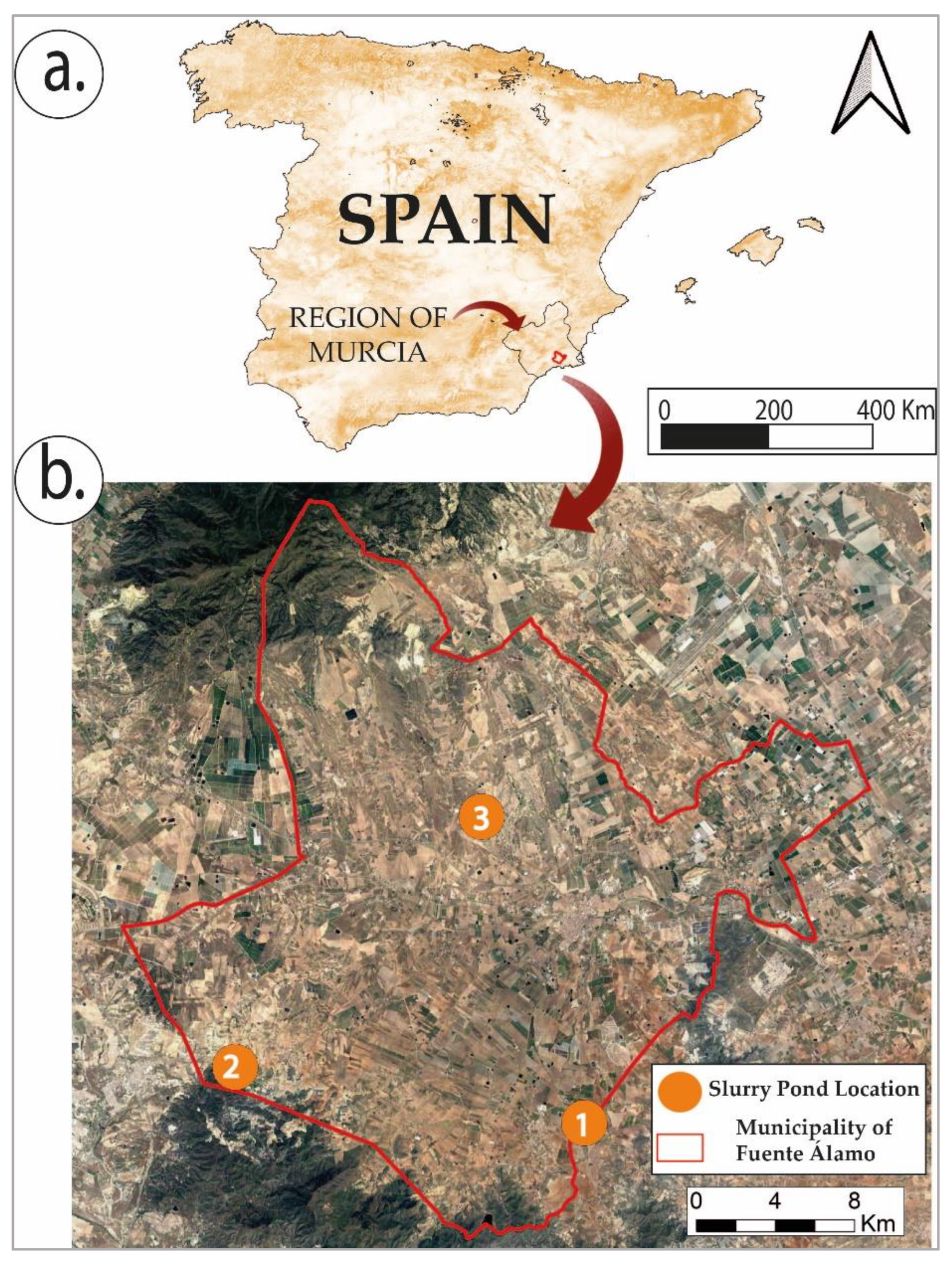
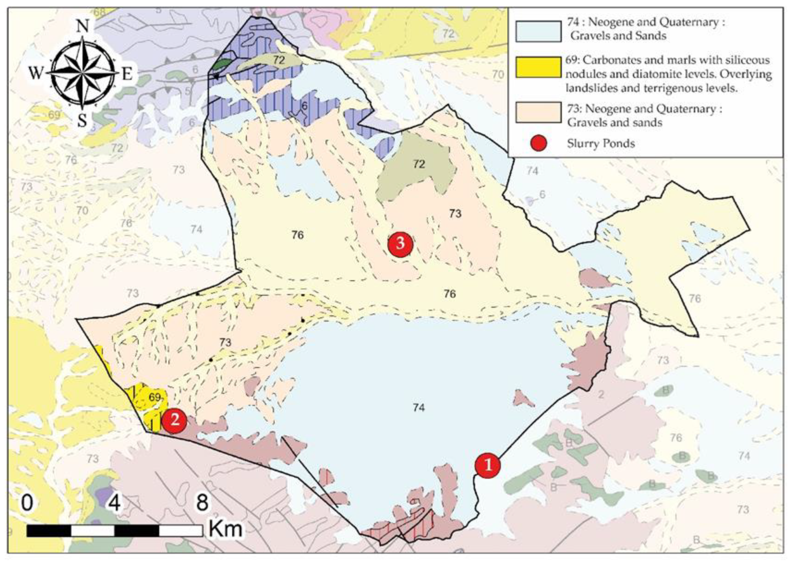
1.1. Study Site
1.2. Pig Slurry Ponds
2. Materials and Methods
- -
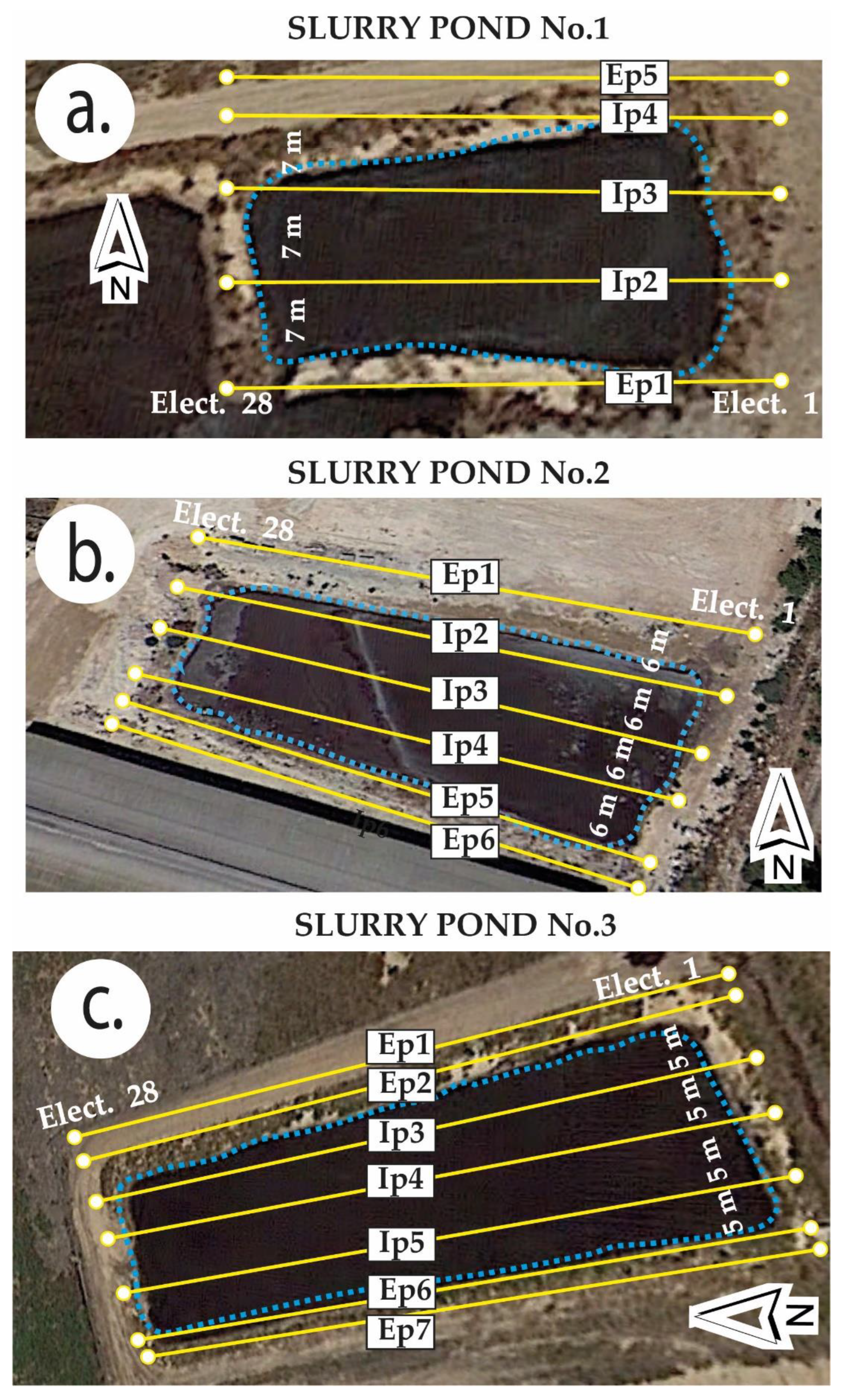
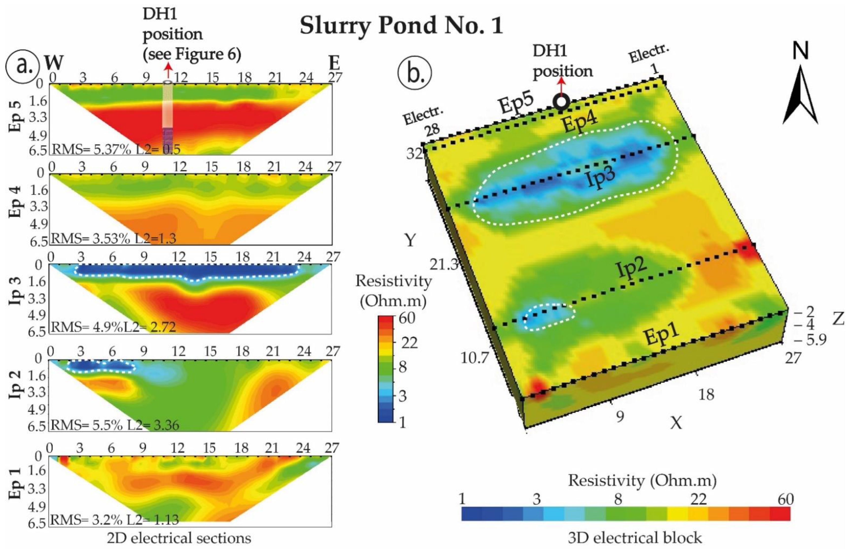
- Five profiles were carried out at slurry pond No. 1. Three of them were external profiles (named Ep1, Ep4, and Ep5, respectively), with one meter between profiles. The other two were internal profiles (labeled Ip2 and Ip3, respectively), with a separation of seven meters between them (Figure 3a).
- -
- Three external profiles were carried out at slurry pond No. 2. Here, external profile No. 1 (Ep1) was placed externally on one side, and the other two external profiles (Ep4 and Ep5) were on the other side (Figure 3b). Additionally, two internal profiles (named Ip2, and Ip3, respectively) were laid out six meters apart (Figure 3b).
- -
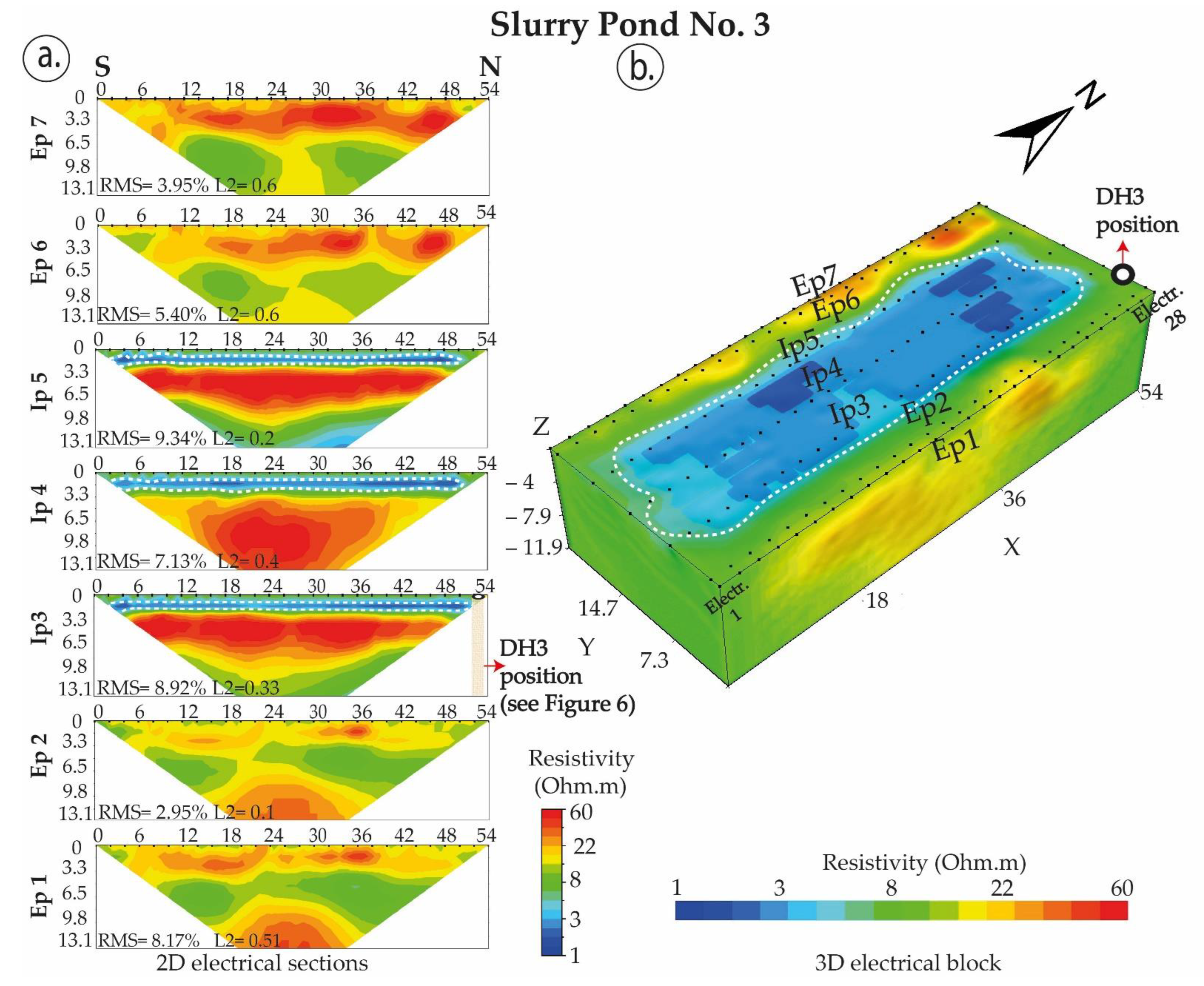
- Seven profiles were carried out at slurry pond No. 3 (Figure 3c). Four of these profiles (Ep1, Ep2, Ep6, and Ep7) were external profiles, where two of them were laid out on one side and the other two on the other side (Figure 3c). Internal ERT profiles (Ip3, Ip4, and Ip5) were laid out with a profile spacing of five meters (Figure 3c).
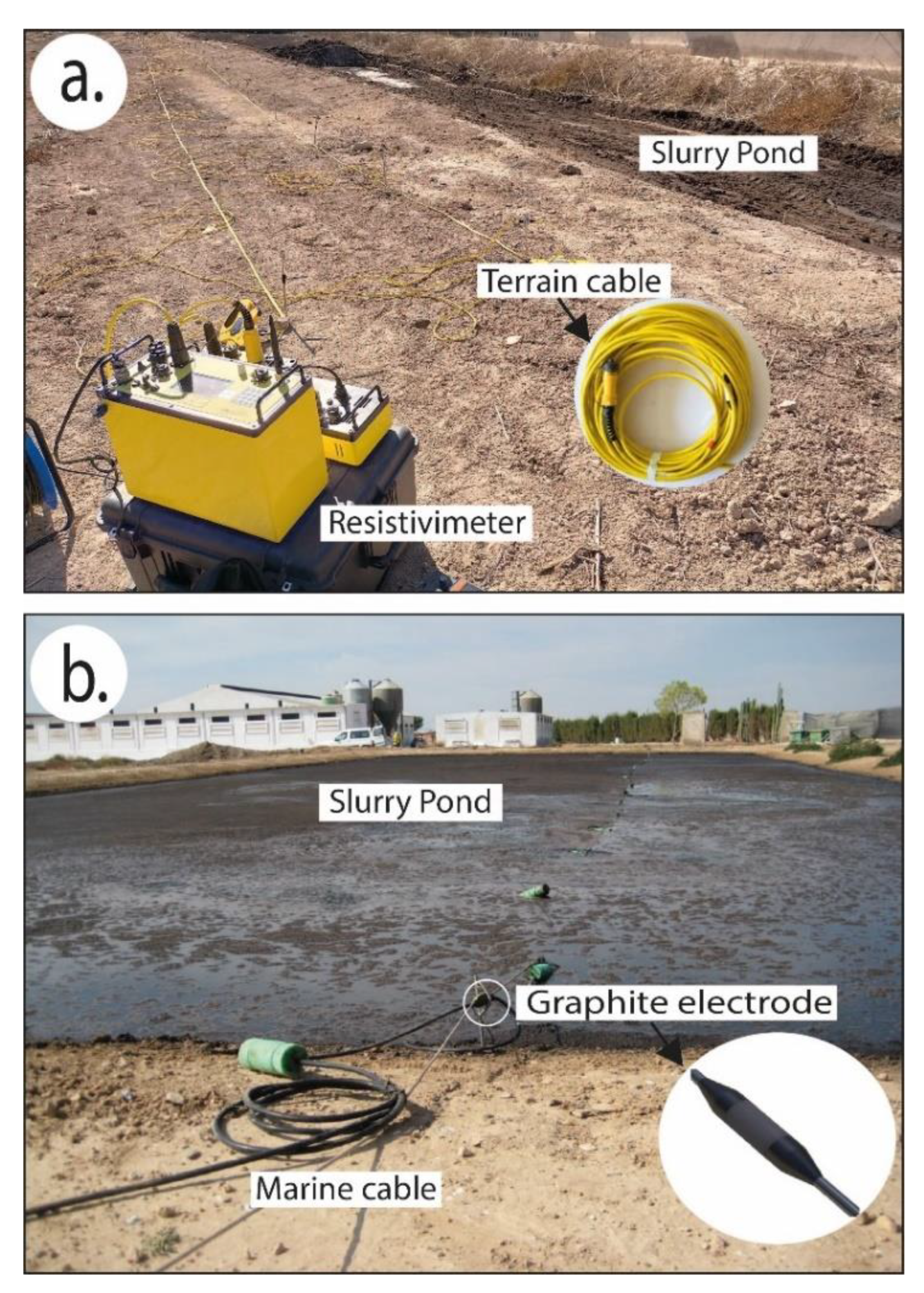
2.1. Electrical Resistivity Tomography (ERT) Method
2.2. Characterization of Soil Properties
2.3. Statistical Analysis
3. Results and Discussion
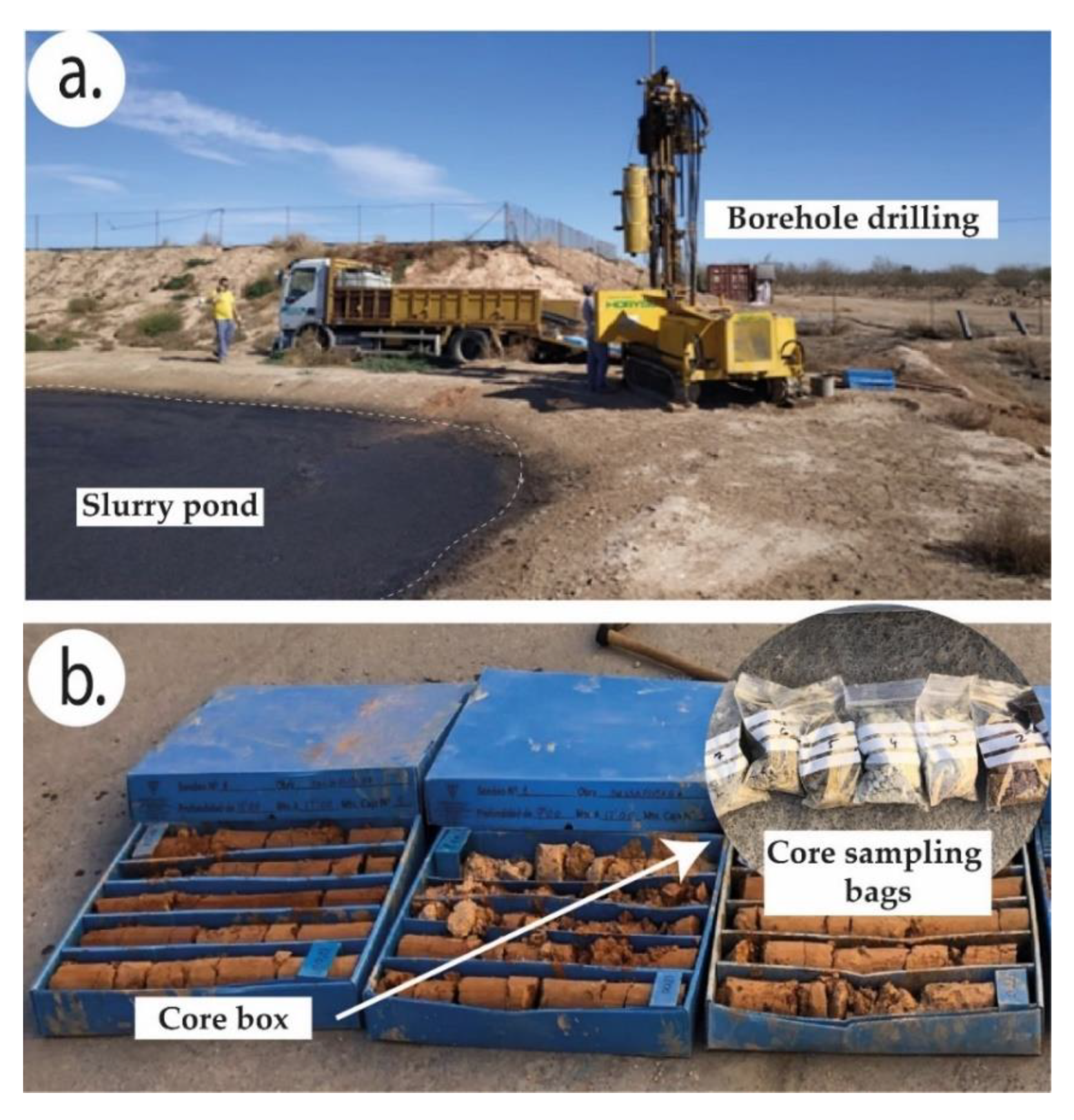
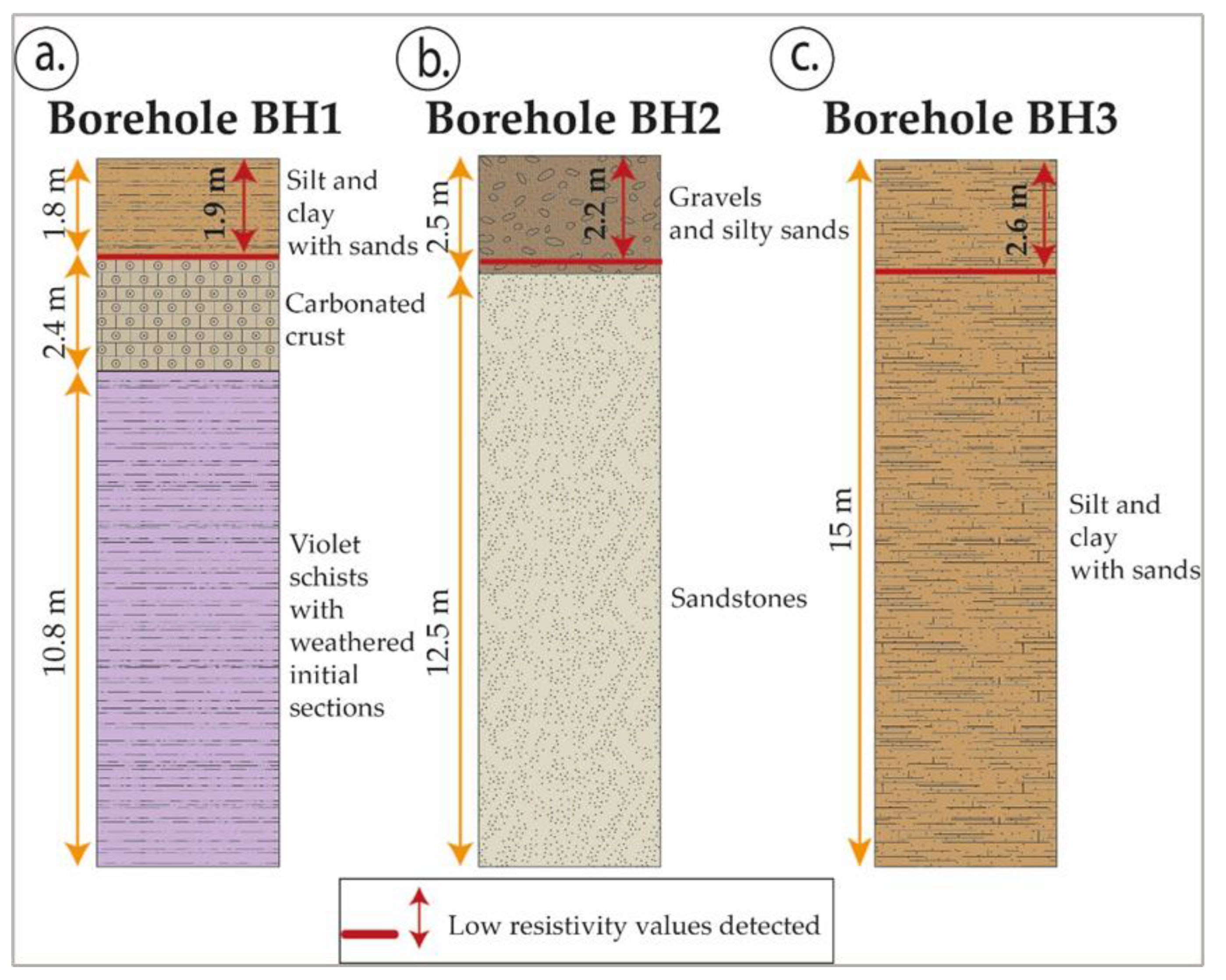
3.1. Borehole Samples and Physicochemical Analyses
3.2. Electrical Resistivity Tomography Models and Statistical Correlations
4. Conclusions
Author Contributions
Funding
Conflicts of Interest
References
- El Sector de la Carne de Cerdo en Cifras: Principales Indicadores Económicos; Subdirección General de Producciones Ganaderas y Cinegéticas and Dirección General de Producciones Mercados Agrarios, Ministerio de Agricultura, Pesca y Alimentación: Madrid, Spain, 2020.
- Caterina, D.; Orozco, A.F.; Nguyen, F. Long-term ERT monitoring of biogeochemical changes of an aged hydrocarbon contamination. J. Contam. Hydrol. 2017, 201, 19–29. [Google Scholar] [CrossRef]
- Martínez-Pagán, P. Aplicación de Diferentes Técnicas no Destructivas de Prospección Geofísica a Problemas Relacionados con Contaminación Ambiental Producida por Diferentes Actividades Antrópicas en la Región de Murcia. Ph.D. Thesis, Universidad Politécnica de Cartagena, Cartagena, Spain, 2006. [Google Scholar]
- Rosales, R.M.; Martinez-Pagan, P.; Faz, A.; Bech, J. Study of subsoil in former petrol stations in SE of Spain: Physicochemical characterization and hydrocarbon contamination assessment. J. Geochem. Explor. 2014, 147, 306–320. [Google Scholar] [CrossRef]
- Acosta, J.A.; Martínez-Pagán, P.; Martínez-Martínez, S.; Faz, A.; Zornoza, R.; Carmona, D.M. Assessment of environmental risk of reclaimed mining ponds using geophysics and geochemical techniques. J. Geochem. Explor. 2014, 147, 80–90. [Google Scholar] [CrossRef]
- Aracil Ávila, E.; Maruri Brouard, U.; Vallés Iriso, J.; Martínez Pagán, P.; Porres Benito, J.A. Evaluación de problemas medioambientales mediante tomografía eléctrica. Geofisica 2003, 122, 34–39. [Google Scholar]
- Allred, B.; Daniels, J.J.; Ehsani, M.R. Handbook of Agricultural Geophysics; CRC Press: Boca Raton, FL, USA, 2008; pp. 211–233. [Google Scholar]
- Samouëlian, A.; Cousin, I.; Tabbagh, A.; Bruand, A.; Richard, G. Electrical resistivity survey in soil science: A review. Soil Tillage Res. 2005, 83, 173–193. [Google Scholar] [CrossRef]
- Chambers, J.E.; Kuras, O.; Meldrum, P.I.; Ogilvy, R.D.; Hollands, J. Electrical resistivity tomography applied to geologic, hydrogeologic, and engineering investigations at a former waste-disposal site. Geophysics 2006, 71, B231–B239. [Google Scholar] [CrossRef]
- Koda, E.; Tkaczyk, A.; Lech, M.; Osiński, P. Application of electrical resistivity data sets for the evaluation of the pollution concentration level within landfill subsoil. Appl. Sci. 2017, 7, 262. [Google Scholar] [CrossRef]
- Yan, Z.; Song, X.; Wu, Y.; Gao, C.; Wang, Y.; Yang, Y. Fingerprinting Organochlorine Groundwater Plumes Based on Non-Invasive ERT Technology at a Chemical Plant. Appl. Sci. 2022, 12, 2816. [Google Scholar] [CrossRef]
- Liao, Q.; Deng, Y.; Shi, X.; Sun, Y.; Duan, W.; Wu, J. Delineation of contaminant plume for an inorganic contaminated site using electrical resistivity tomography: Comparison with direct-push technique. Environ. Monit. Assess. 2018, 190, 187. [Google Scholar] [CrossRef]
- Sainato, C.M.; Losinno, B.N.; Malleville, H.J. Assessment of contamination by intensive cattle activity through electrical resistivity tomography. J. Appl. Geophys. 2012, 76, 82–91. [Google Scholar] [CrossRef]
- Sendrós, A.; Urruela, A.; Himi, M.; Alonso, C.; Lovera, R.; Tapias, J.C.; Casas, A. Characterization of a shallow coastal aquifer in the framework of a subsurface storage and soil aquifer treatment project using electrical resistivity tomography (Port de la Selva, Spain). Appl. Sci. 2021, 11, 2448. [Google Scholar] [CrossRef]
- Netto, L.G.; Barbosa, A.M.; Galli, V.L.; Pereira, J.P.S.; Gandolfo, O.C.B.; Birelli, C.A. Application of invasive and non-invasive methods of geo-environmental investigation for determination of the contamination behavior by organic compounds. J. Appl. Geophys. 2020, 178, 104049. [Google Scholar] [CrossRef]
- Simyrdanis, K.; Papadopoulos, N.; Soupios, P.; Kirkou, S.; Tsourlos, P. Characterization and monitoring of subsurface contamination from Olive Oil Mills’ waste waters using Electrical Resistivity Tomography. Sci. Total Environ. 2018, 637, 991–1003. [Google Scholar] [CrossRef]
- Sainato, C.M.; Losinno, B.N.; Malleville, H.J. Electrical resistivity tomography applied to detect contamination on a dairy farm in the Pampean region, Argentina. Near Surf. Geophys. 2010, 8, 163–171. [Google Scholar] [CrossRef]
- Lemeillet, F.; Sainato, C.; Malleville, H.; Carbó, L.; Herrero, A. Electrical conductivity of a soil treated with effluent from livestock. Geoacta 2016, 41, 57–73. [Google Scholar]
- Martínez-Pagán, P.; Faz, A.; Aracil, E. The use of 2D electrical tomography to assess pollution in slurry ponds of the Murcia region, SE Spain. Near Surf. Geophys. 2009, 7, 49–61. [Google Scholar] [CrossRef]
- Sánchez, D.E. Riesgo de heladas por inversión térmica en la huerta de Murcia: Incidencia en la actividad agraria. Investig. Geográficas (Esp) 2015, 64, 73–86. [Google Scholar] [CrossRef]
- Marín Lechado, C.; Roldán García, F.J.; Pineda Velasco, A.; Martínez Zubieta, P.; Rodero Pérez, J.; Diaz Pinto, G. Mapa Geológico continuo de España 1:50,000 Zonas internas de las cordilleras béticas (Zona-2210) in GEODE. In Mapa Geológico Digital Continuo de España [En Línea]; Instituto Geológico y MInero de España: Madrid, Spain, 2008. [Google Scholar]
- Confederación Hidrográfica del Segura. Plan Hidrológico de la Demarcación del Segura 2015/21; Caracterización de las Masas de Agua de la DHS: Madrid, Spain, 2015. [Google Scholar]
- Estrella, T.R. Funcionamiento hidrogeológico del campo de Cartagena (Murcia y Alicante). Hidrogeología 1995, 11, 21–38. [Google Scholar]
- Lobera, J.B.; Martínez, P.; Ferrández, F.; Martín, J. Reutilización Agronómica de los Purines de Cerdo; Serie técnica y de estudios; Consejería de Medio Ambiente, Agricultura y Agua: Murcia, Spain, 1998. [Google Scholar]
- Binley, A.; Slater, L. Resistivity and Induced Polarization. In Resistivity and Induced Polarization; Cambridge University Press: Cambridge, UK, 2020; p. 426. [Google Scholar]
- Martínez-Segura, M.A.; Vásconez-Maza, M.D.; García-Nieto, M.C. Volumetric characterisation of waste deposits generated during the production of fertiliser derived from phosphoric rock by using LiDAR and electrical resistivity tomography. Sci. Total Environ. 2020, 716, 137076. [Google Scholar] [CrossRef]
- Martín-Crespo, T.; Gómez-Ortiz, D.; Martínez-Pagán, P.; De Ignacio-San José, C.; Martín-Velázquez, S.; Lillo, J.; Faz, A. Geoenvironmental characterization of riverbeds affected by mine tailings in the Mazarrón district (Spain). J. Geochem. Explor. 2012, 119, 6–16. [Google Scholar] [CrossRef]
- Cano, Á.F.; Martínez-Pagán, P.; Ávila, E.A.; Brouard, U.M. Aplicación de la tomografía eléctrica al estudio de los depósitos de estériles mineros “El Lirio” y “Brunita” (Murcia). In Los Residuos Minero-Metalúrgicos en el Medio Ambiente; Instituto Geológico y Minero de España (IGME): Madrid, Spain, 2006; p. 89. [Google Scholar]
- Martínez-Pagán, P.; Gómez-Ortiz, D.; Martín-Crespo, T.; Martín-Velázquez, S.; Martínez-Segura, M. Electrical resistivity imaging applied to tailings ponds: An overview. Mine Water Environ. 2021, 40, 285–297. [Google Scholar] [CrossRef]
- Constable, S.C.; Parker, R.L.; Constable, C.G. Occam’s inversion: A practical algorithm for generating smooth models from electromagnetic sounding data. Geophysics 1987, 52, 289–300. [Google Scholar] [CrossRef]
- DeGroot-Hedlin, C.; Constable, S. Occam’s inversion to generate smooth, two-dimensional models from magnetotelluric data. Geophysics 1990, 55, 1613–1624. [Google Scholar] [CrossRef]
- Instruction Manual for EarthImager 3D Version 1.5.3 Resistivity Inversion Software; Advanced Geosciences Inc.: Austin, TX, USA, 2008; p. 100.
- Yang, X.; Lagmanson, M.; Yang, X.; Lagmanson, M. Comparison of 2D and 3D Electrical Resistivity Imaging Methods. En Symposium on the Application of Geophysics to Engineering and Environmental Problems 2006; Society of Exploration Geophysicists: Houston, TX, USA, 2006; pp. 585–594. [Google Scholar]
- Cobertera, E. Edafología Aplicada, 1st ed.; Ediciones Cátedra, S.A.: Madrid, Spain, 1993; p. 326. [Google Scholar]
- Andrades, M. Prácticas de Edafología y Climatología; Universidad de la Rioja: Logroño, Spain, 1996; pp. 14–16. Available online: https://dialnet.unirioja.es/descarga/libro/194611.pdf (accessed on 18 September 2021).
- Martínez-Pagán, P.; Cano, Á.F.; Ramos da Silva, G.R.; Olivares, A.B. 2-D electrical resistivity imaging to assess slurry pond subsoil pollution in the southeastern region of Murcia, Spain. J. Environ. Eng. Geophys. 2010, 15, 29–47. [Google Scholar] [CrossRef]
- Straczynska, S. The influence of fertilizing with manure on the soil acidity. Zesz. Probl. Postępów Nauk. Rol. 1994, 413, 283–285. [Google Scholar]
- Chang, C.; Sommerfeldt, T.G.; Entz, T. Rates of soil chemical changes with eleven annual applications of cattle feedlot manure. Can. J. Soil Sci. 1990, 70, 673–681. [Google Scholar] [CrossRef]
- Pozdnyakov, A.I.; Pozdnyakova, L.A.; Karpachevskii, L.O. Relationship between water tension and electrical resistivity in soils. Eurasian Soil Sci. 2006, 39, S78–S83. [Google Scholar] [CrossRef]
- Peralta, N.R.; Cicore, P.L.; Marino, M.A.; da Silva, J.R.M.; Costa, J.L. Use of geophysical survey as a predictor of the edaphic properties variability in soils used for livestock production. Span. J. Agric. Res. 2015, 13, e1103. [Google Scholar] [CrossRef]
- Carrasco, M.; Cecilia, L. Utilización Agronómica de Purines de Cerdo en Brócoli y Sandía en Condiciones Mediterráneas Semiáridas: Influencia en el Sistema Suelo-Planta. Ph.D. Thesis, Universidad Politécnica de Cartagena, Cartagena, Spain, 2005. [Google Scholar]
- Carnol, M.; Ineson, P.; Anderson, J.M.; Beese, F.; Berg, M.P.; Bolger, T.; Verhoef, H.A. The effects of ammonium sulphate deposition and root sinks on soil solution chemistry in coniferous forest soils. Biogeochemistry 1997, 38, 255–280. [Google Scholar] [CrossRef]
- Bernal, M.P.; Roig, A.; Madrid, R.; Navarro, A.F. Salinity risks on calcareous soils following pig slurry applications. Soil Use Manag. 1992, 8, 125–129. [Google Scholar] [CrossRef]
- Heiniger, R.W.; McBride, R.G.; Clay, D.E. Using soil electrical conductivity to improve nutrient management. Agron. J. 2003, 95, 508–519. [Google Scholar] [CrossRef]
- Mazaheri, M.R.; Mahmoodabadi, M. Study on infiltration rate based on primary particle size distribution data in arid and semiarid region soils. Arab. J. Geosci. 2012, 5, 1039–1046. [Google Scholar] [CrossRef]
- Oster, J.D.; Shainberg, I. Soil responses to sodicity and salinity: Challenges and opportunities. Soil Res. 2001, 39, 1219–1224. [Google Scholar] [CrossRef]
- Bronick, C.J.; Lal, R. Soil structure and management: A review. Geoderma 2005, 124, 3–22. [Google Scholar] [CrossRef]
- Garcia, G.N. Química Agrícola: El Suelo y los Elementos Químicos: El Suelo y los Elementos Químicos Esenciales Para la Vida Vegetal, 2nd ed.; Mundi-Prensa Libros: Madrid, Spain, 2003. [Google Scholar]
- Mantovi, P.; Fumagalli, L.; Beretta, G.P.; Guermandi, M. Nitrate leaching through the unsaturated zone following pig slurry applications. J. Hydrol. 2006, 316, 195–212. [Google Scholar] [CrossRef]
- Daudén, A.; Quılez, D. Pig slurry versus mineral fertilization on corn yield and nitrate leaching in a Mediterranean irrigated environment. Eur. J. Agron. 2004, 21, 7–19. [Google Scholar] [CrossRef]
- Piñeiro, C.; Montalvo, G. La Directiva IPPC Para el Control Integrado de las Emisiones Contaminantes en Ganadería Intensiva de Porcino; XXI Curso de Especialización FEDNA; En Avances en Nutrición y Alimentación Animal; Fundación Española para el Desarrollo de la Nutrición Animal: Madrid, Spain, 2005; Volume 7, pp. 81–86. [Google Scholar]
- Hernandez, R.; Jonathan, O. Determinación de Propiedades de Suelos Agrícolas a Partir de Mediciones Eléctricas Realizadas en Campo y Laboratorio. Master’s Thesis, Instituto Potosino de Investigación Científica y Tecnológica, A.C., San Luis Potosi, Mexico, 2019. [Google Scholar]
- Dionisi, C.P.; Mignone, R.A.; Rubenacker, A.I.; Pfaffen, V.; Bachmeier, O.; Campitelli, P.A.; Juarez, A.V. Monitoring of physicochemical parameters of soils after applying pig slurry. Analysis of its application in short and long periods in the province of Córdoba, Argentina. Microchem. J. 2020, 159, 105545. [Google Scholar] [CrossRef]
- Siddiqui, F.I.; Osman, S.B.A.B.S. Simple and multiple regression models for relationship between electrical resistivity and various soil properties for soil characterization. Environ. Earth Sci. 2013, 70, 259–267. [Google Scholar] [CrossRef]
- Michot, D.; Benderitter, Y.; Dorigny, A.; Nicoullaud, B.; King, D.; Tabbagh, A. Spatial and temporal monitoring of soil water content with an irrigated corn crop cover using surface electrical resistivity tomography. Water Resour. Res. 2003, 39, 1138. [Google Scholar] [CrossRef]


| Slurry Pond No. 1 | |||||||||||
| Depth | Moisture | pH | EC (dS/m) | Cl− | SO42− (mg/kg) | Na+ (mg/kg) | Mg2+ (mg/kg) | N-NO3− (mg/kg) | Clay | Silt | Sand |
| (m) | (%) | (mg/kg) | % | % | % | ||||||
| −1.00 | 10.66 | 8.20 | 0.80 | 657.26 | 58.63 | 160.97 | 49.07 | 97.60 | 9 | 37 | 55 |
| −1.80 | 15.97 | 8.49 | 0.37 | 234.12 | 58.74 | 66.76 | 51.26 | 45.05 | 20 | 68 | 13 |
| −3.00 | 7.47 | 9.03 | 0.16 | 24.98 | 37.63 | 19.99 | 13.07 | 2.80 | 10 | 65 | 26 |
| Slurry Pond No. 2 | |||||||||||
| Depth | Moisture | pH | EC (dS/m) | Cl− | SO42− (mg/kg) | Na+ (mg/kg) | Mg2+ (mg/kg) | N-NO3− (mg/kg) | Clay | Silt | Sand |
| (m) | (%) | (mg/kg) | % | % | % | ||||||
| −1.00 | 17.72 | 8.24 | 3.75 | 5644.25 | 2897.67 | 2544.33 | 1337.70 | 951.90 | 3 | 49 | 49 |
| −2.20 | 16.32 | 8.16 | 2.72 | 1559.65 | 1233.43 | 812.85 | 137.84 | 746.83 | 6 | 42 | 52 |
| −3.00 | 14.53 | 8.54 | 1.42 | 1154.21 | 1059.64 | 553.02 | 74.37 | 423.32 | 3 | 42 | 55 |
| Slurry Pond No. 3 | |||||||||||
| Depth | Moisture | pH | EC (dS/m) | Cl− | SO42− (mg/kg) | Na+ (mg/kg) | Mg2+ (mg/kg) | N-NO3− (mg/kg) | Clay | Silt | Sand |
| (m) | (%) | (mg/kg) | % | % | % | ||||||
| −1.50 | 6.02 | 8.31 | 0.81 | 267.03 | 885.18 | 257.40 | 82.70 | 143.29 | 12 | 47 | 41 |
| −2.10 | 10.13 | 8.89 | 0.13 | 77.70 | 112.77 | 73.49 | 25.36 | 9.38 | 9 | 54 | 37 |
| −4.20 | 6.21 | 8.77 | 0.16 | 0.00 | 191.03 | 53.63 | 23.68 | 1.93 | 9 | 53 | 39 |
Publisher’s Note: MDPI stays neutral with regard to jurisdictional claims in published maps and institutional affiliations. |
© 2022 by the authors. Licensee MDPI, Basel, Switzerland. This article is an open access article distributed under the terms and conditions of the Creative Commons Attribution (CC BY) license (https://creativecommons.org/licenses/by/4.0/).
Share and Cite
Capa-Camacho, X.; Martínez-Pagán, P.; Martínez-Segura, M.A.; Gabarrón, M.; Faz, Á. Delimiting Pig Slurry Affected Subsurface Areas by Combining Geophysical and Geochemical Techniques. Water 2022, 14, 1872. https://doi.org/10.3390/w14121872
Capa-Camacho X, Martínez-Pagán P, Martínez-Segura MA, Gabarrón M, Faz Á. Delimiting Pig Slurry Affected Subsurface Areas by Combining Geophysical and Geochemical Techniques. Water. 2022; 14(12):1872. https://doi.org/10.3390/w14121872
Chicago/Turabian StyleCapa-Camacho, Ximena, Pedro Martínez-Pagán, Marcos A. Martínez-Segura, María Gabarrón, and Ángel Faz. 2022. "Delimiting Pig Slurry Affected Subsurface Areas by Combining Geophysical and Geochemical Techniques" Water 14, no. 12: 1872. https://doi.org/10.3390/w14121872
APA StyleCapa-Camacho, X., Martínez-Pagán, P., Martínez-Segura, M. A., Gabarrón, M., & Faz, Á. (2022). Delimiting Pig Slurry Affected Subsurface Areas by Combining Geophysical and Geochemical Techniques. Water, 14(12), 1872. https://doi.org/10.3390/w14121872