
Failure of the Downstream Shoulder of Rockfill Dams Due to Overtopping or Throughflow


Abstract
1. Introduction
2. Methodology
2.1. Test Overview
2.2. Specific Tests
- [Group A]: , , , , Gravel M5 (tests 5, 6, 7).
- [Group B]: , , , , Gravel M7 (tests 8, 9).
- [Group C]: , , , , Gravel M6 (tests 81, 82, 85, 87, 88).
- [Group D]: , , , , Gravel M6 (tests 89, 90, 91, 92).
- [Group E]: , , , , Gravel M6 (tests 94, 95).
2.3. Test Setup and Procedure
2.4. Materials
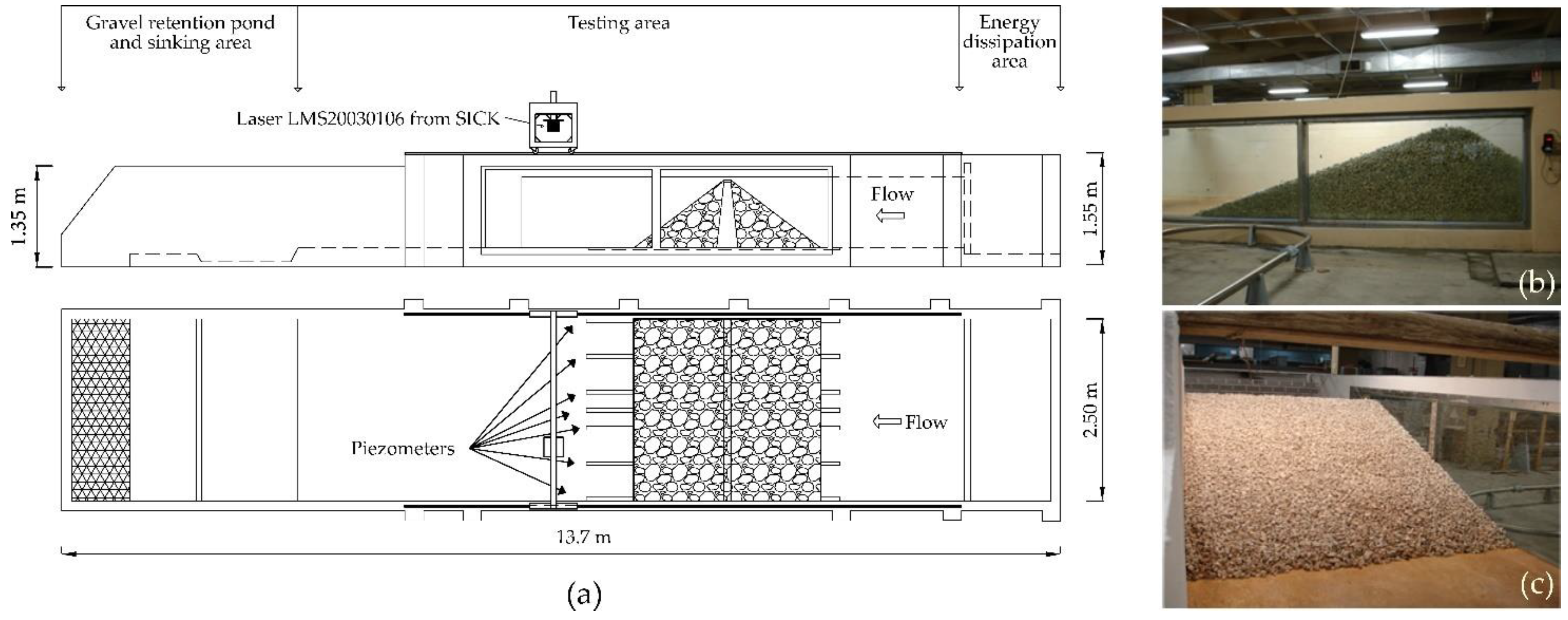
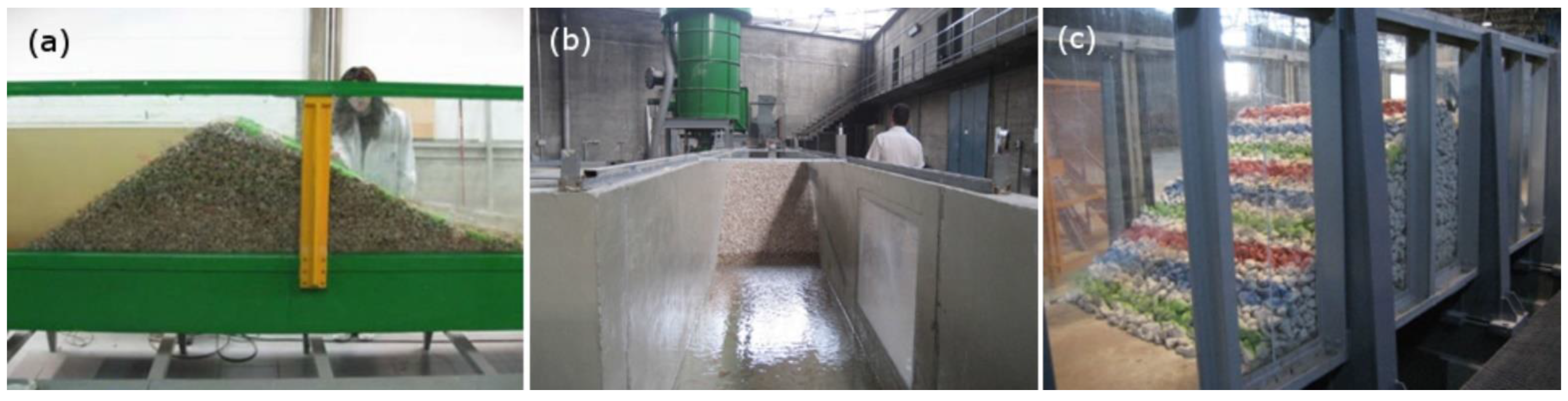
2.5. Facilities and Instrumentation
2.6. Dimensionless Variables
2.7. Statistical Analyses
3. Results
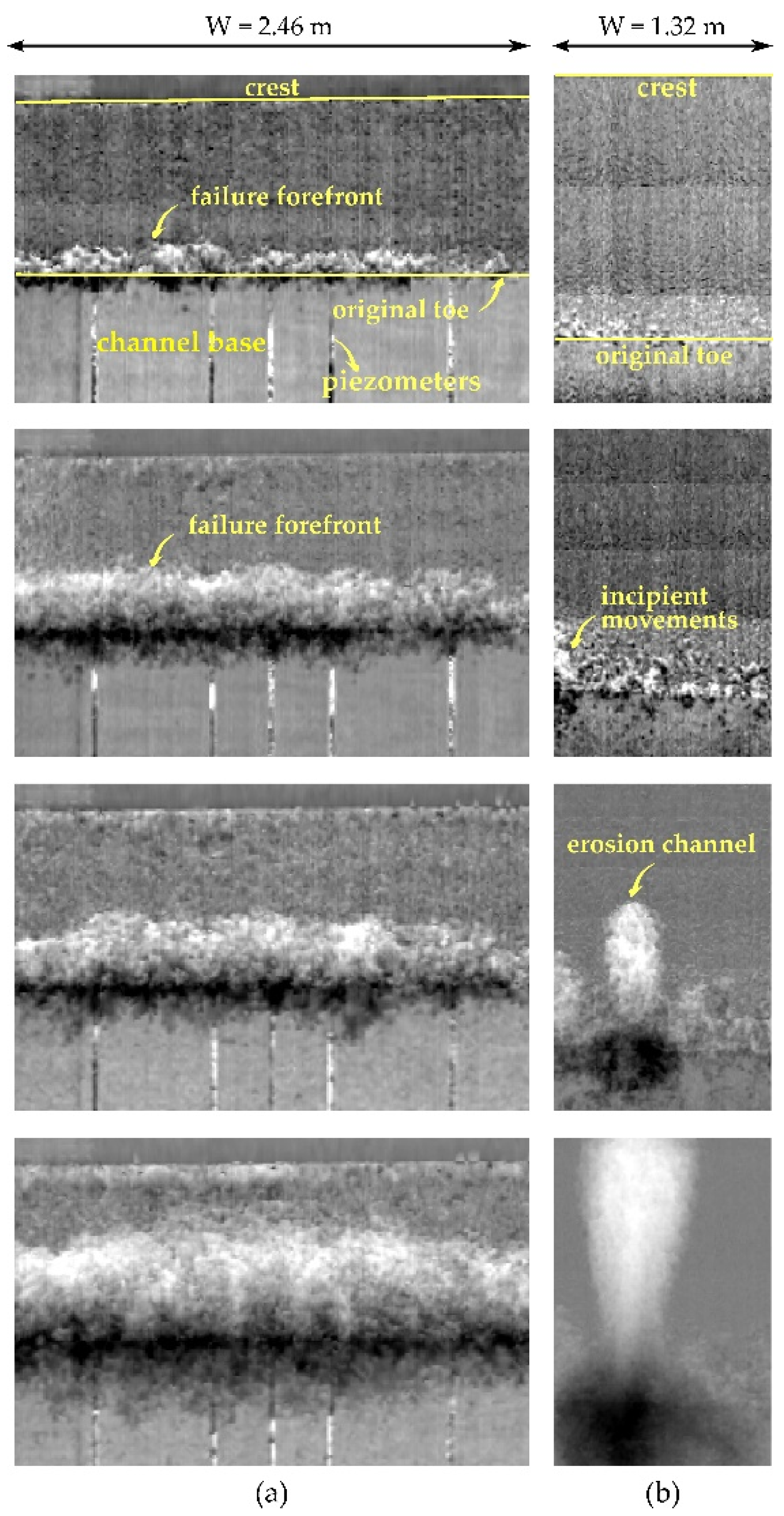
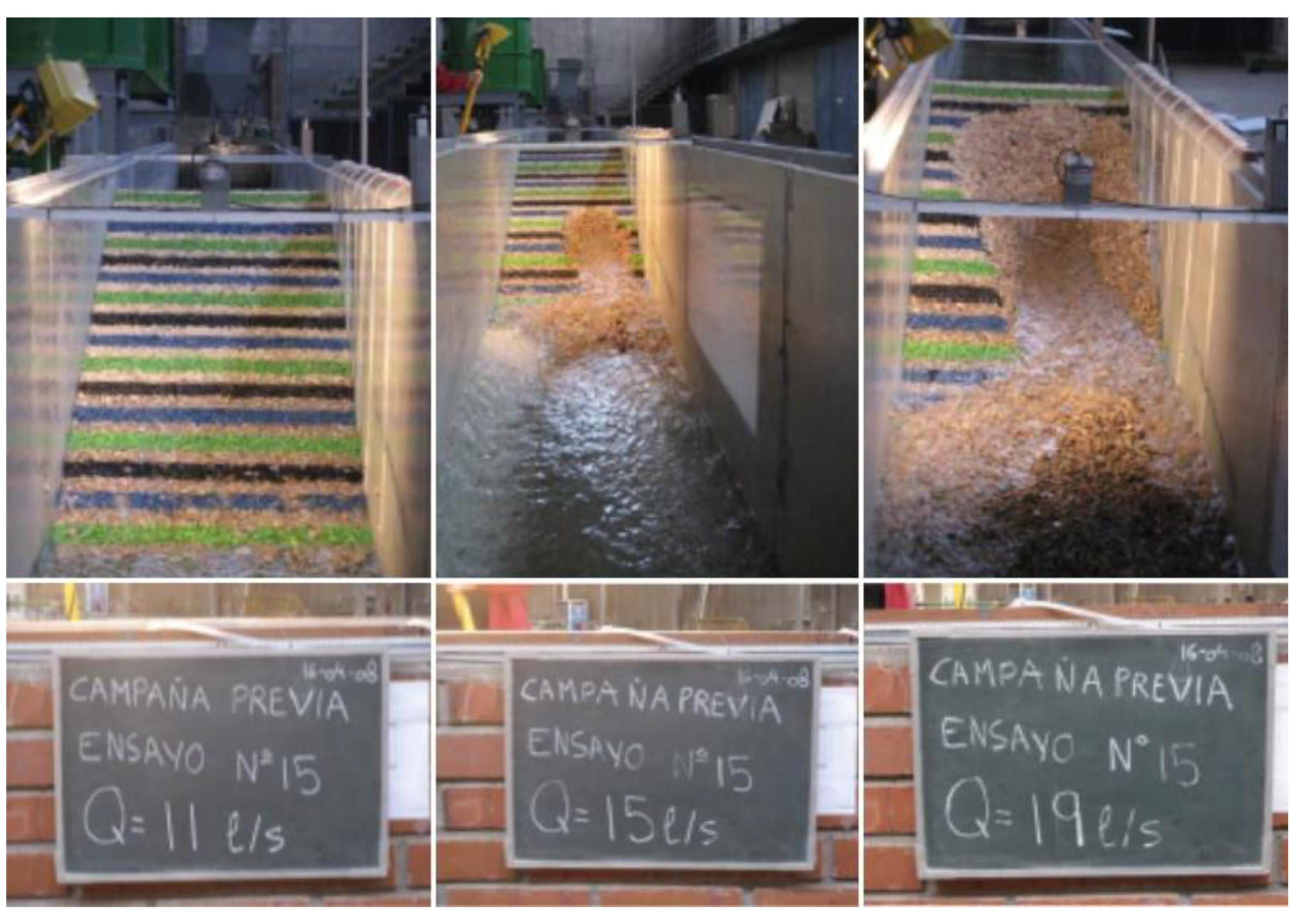
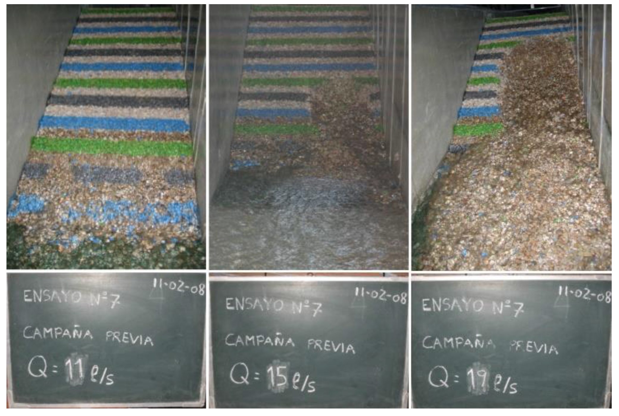
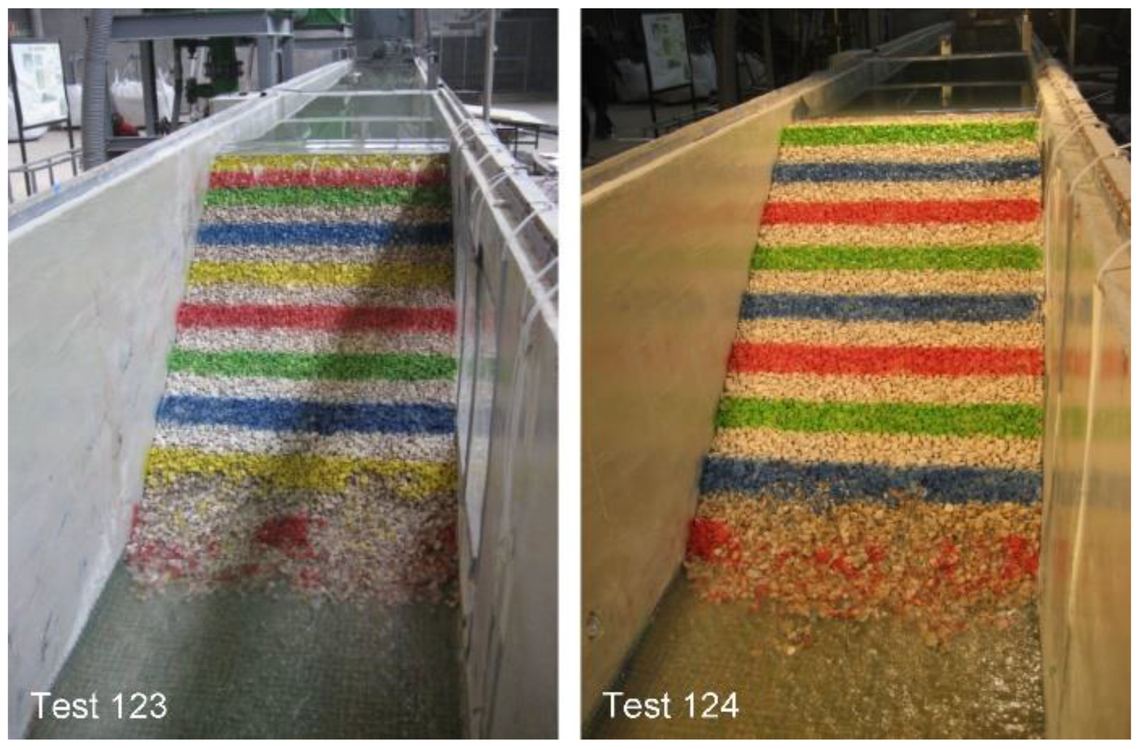
3.1. Failure Initiation and Progress
3.2. Failure Discharge
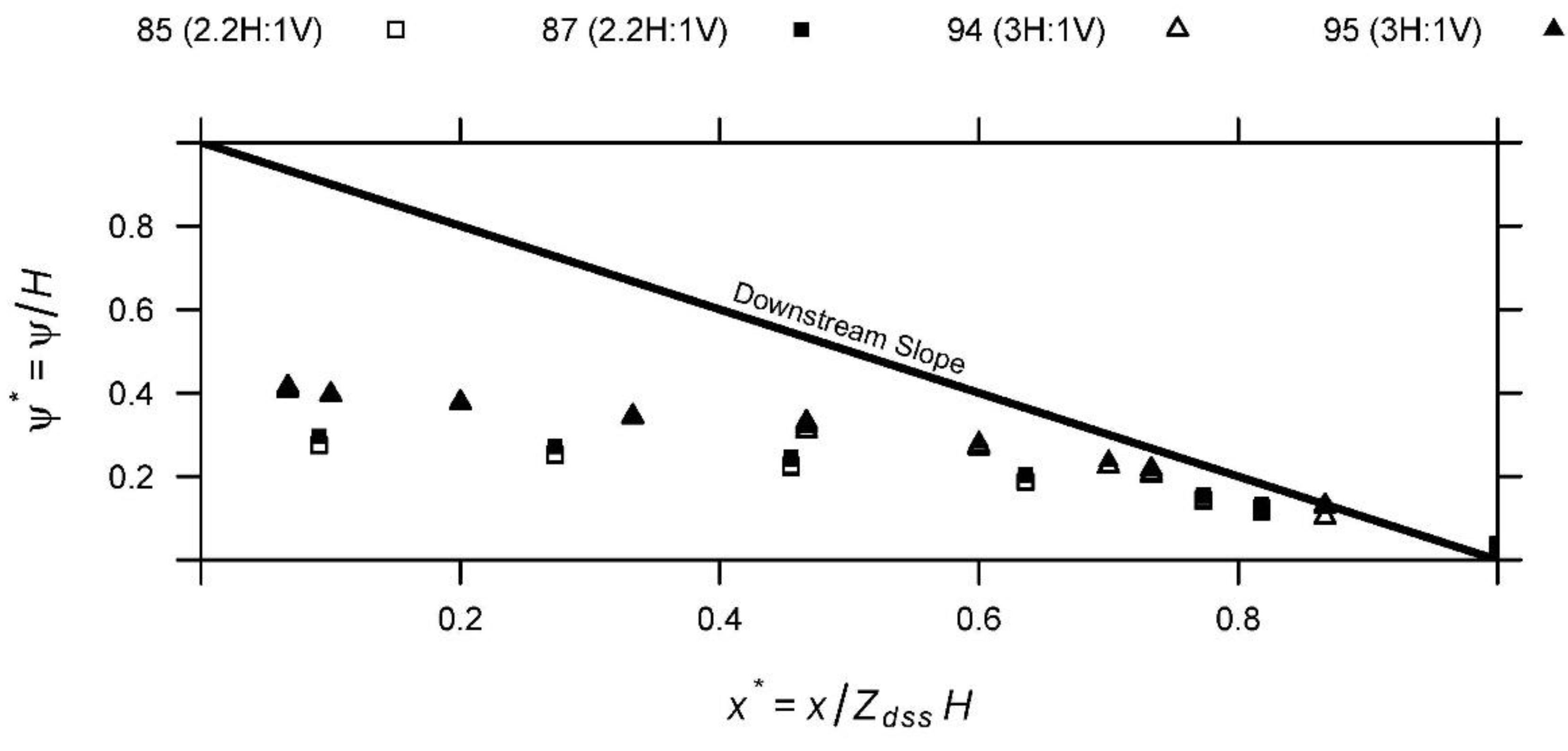
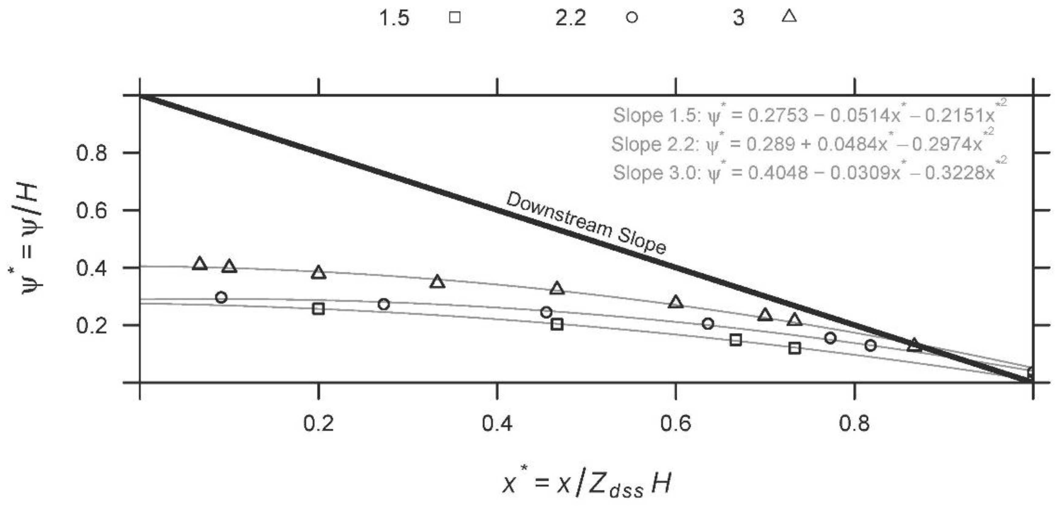
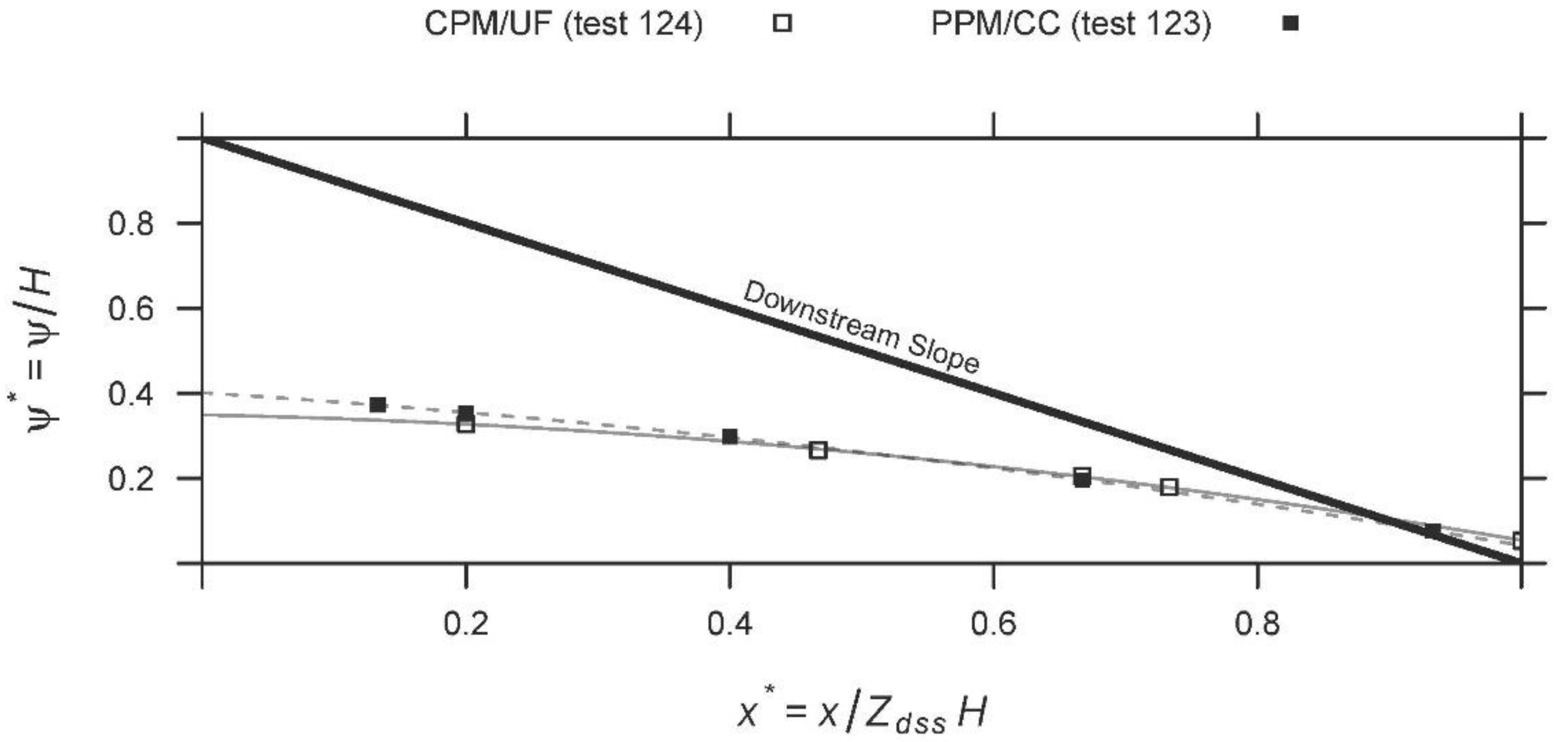
3.3. Hydraulic Pressures
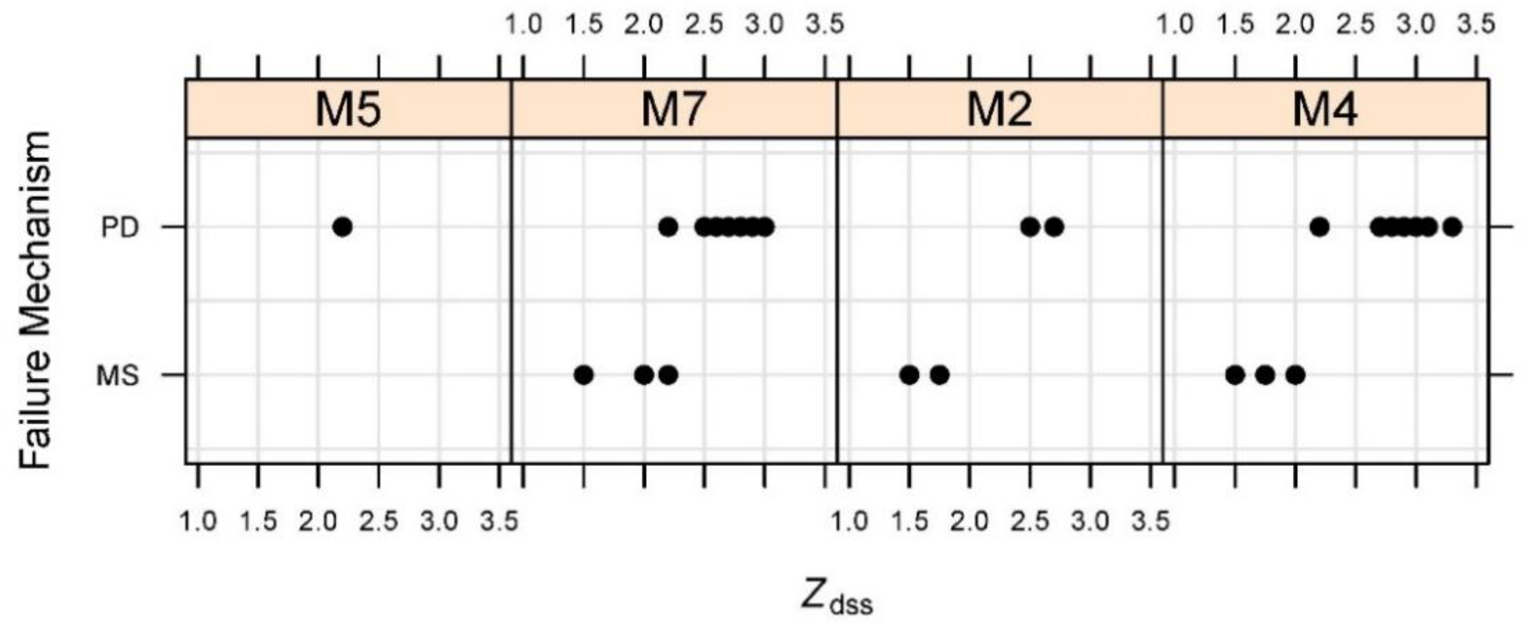
3.4. Failure Mechanisms
4. Discussion
4.1. The Mechanics of Failure
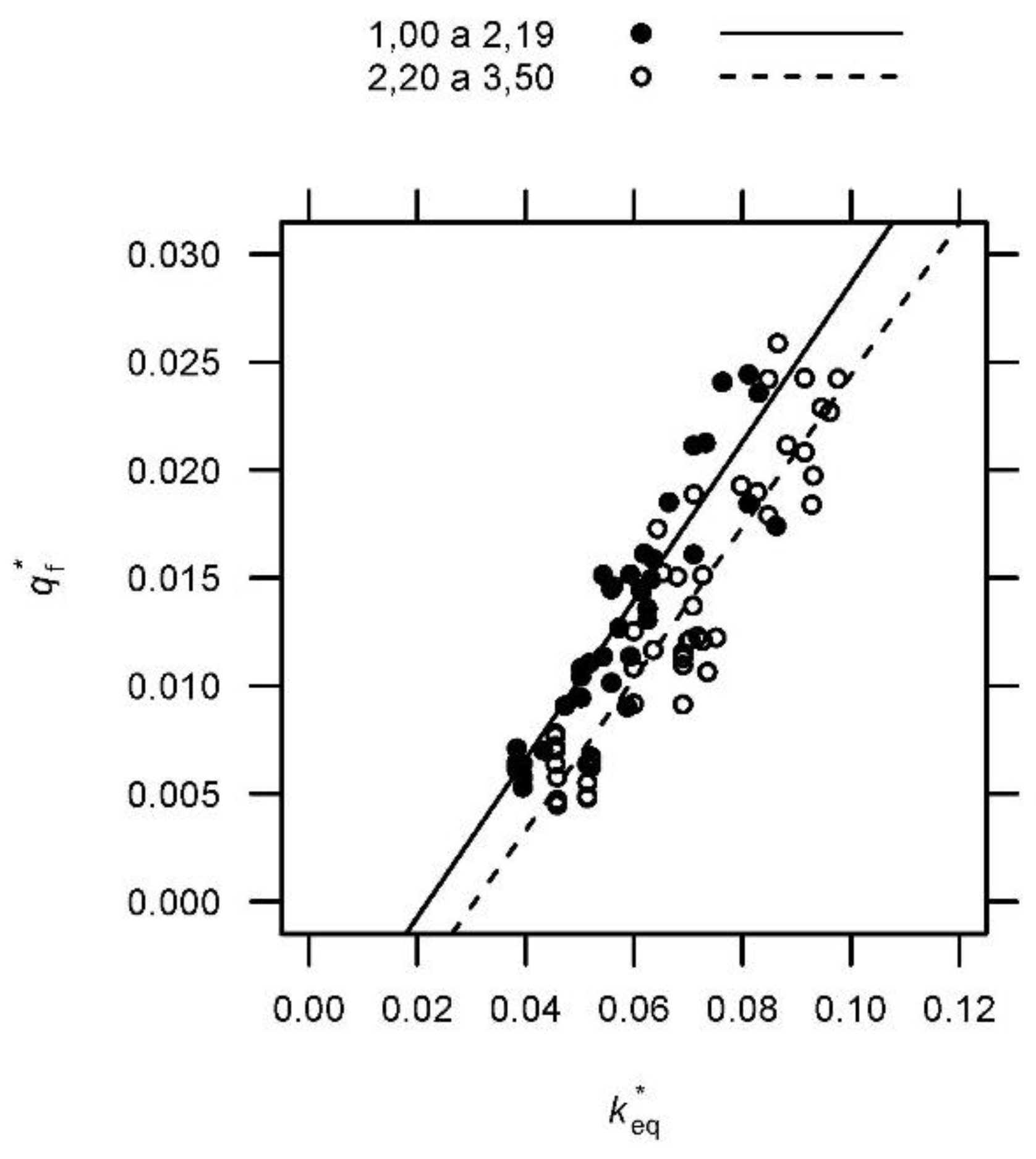
4.2. The Scale Effect
4.3. Repeatability
4.4. The Effect of the Downstream Slope
4.5. Other Effects
4.6. Research Scope and Limitations
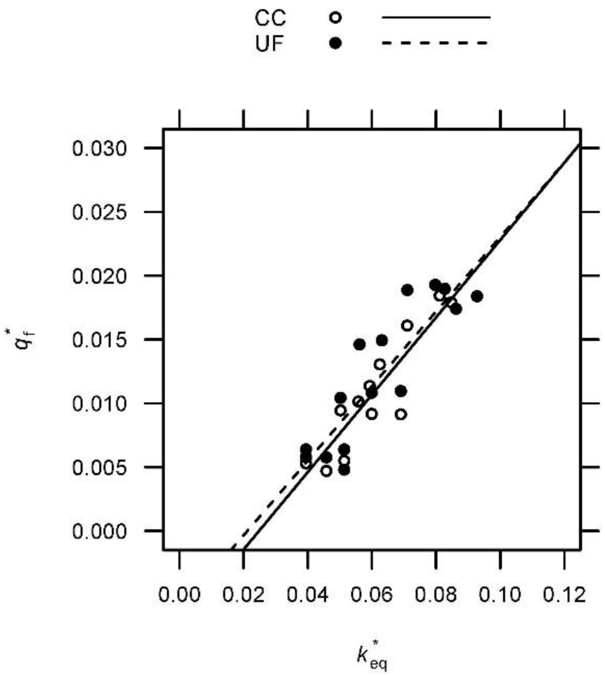
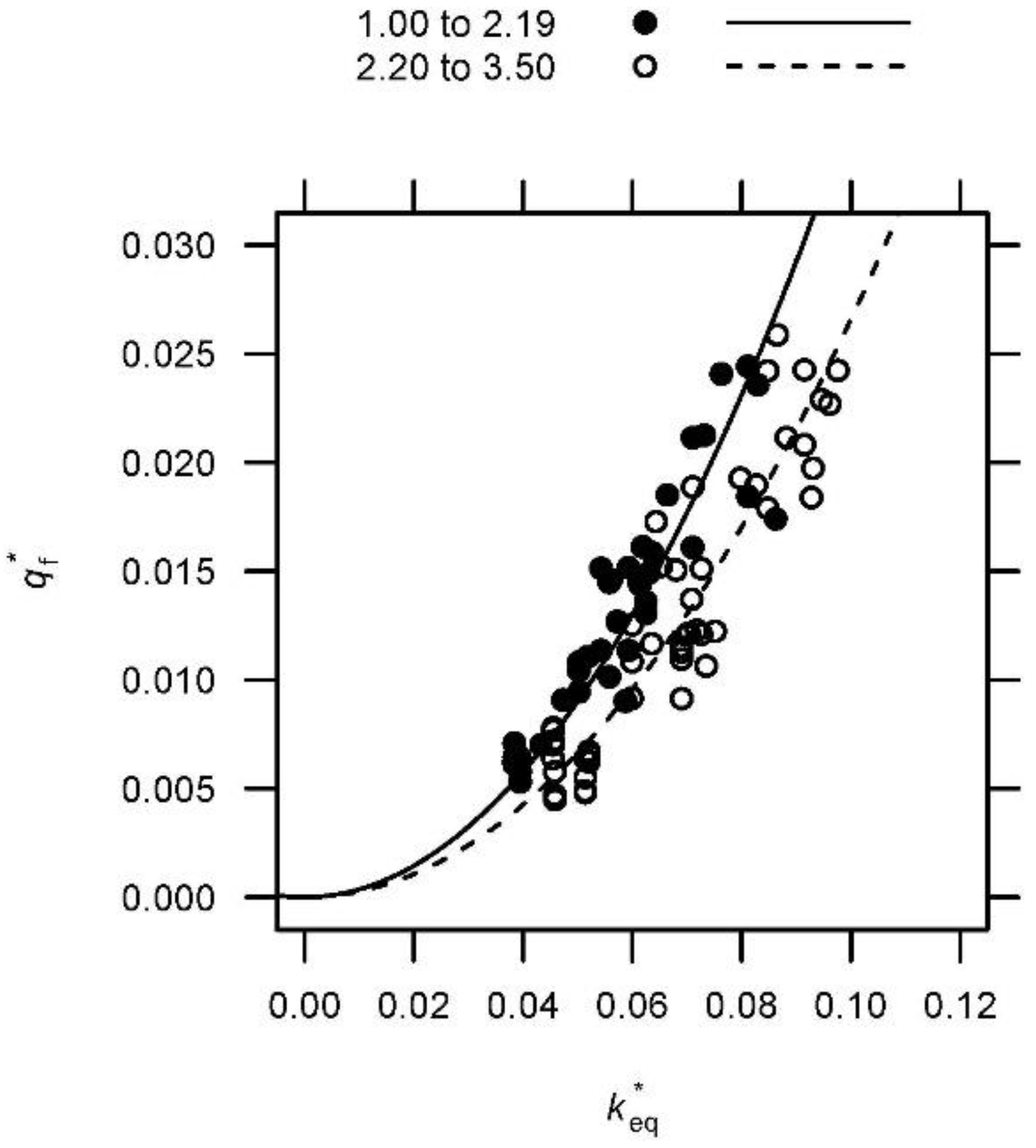
4.7. A Regression Model for the Failure Discharge
5. Conclusions
Author Contributions
Funding
Acknowledgments
Conflicts of Interest
Nomenclature
| a | Seepage resistance coefficient of the quadratic flow equation (fundamental units T·L−1) |
| b | Seepage resistance coefficient of the quadratic flow equation (fundamental units T2·L−2) |
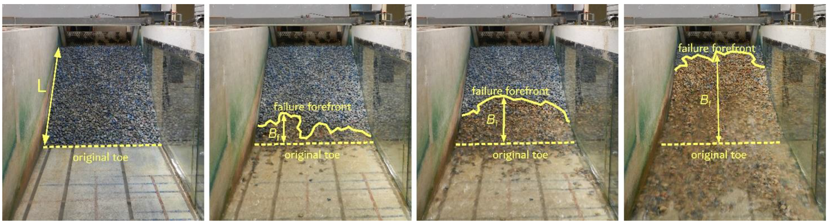
| Bf | Maximum advance of failure in relation to the embankment toe, i.e., the distance between the most upward point of the failure forefront and the downstream toe as shown in Figure 2 (fundamental units L) |
| CC | Central core |
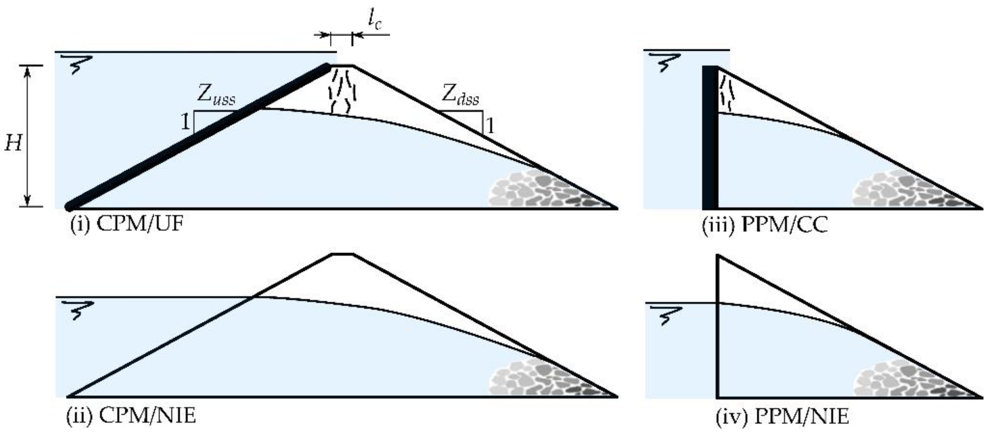
| CPM | Complete physical model or complete configuration (both upstream and downstream slopes and crest) |
| CPM/UF | Complete configuration with upstream face |
| CPM/NIE | Complete configuration without impervious element |
| Cu | Coefficient of uniformity, the ratio where and are the sieve sizes through which and of the granular material (dimensionless) passes |
| CV | Coefficient of variation |
| D50 | Sieve size passing 50% of the particles (fundamental units L) |
| DSS | Downstream shoulder |
| e | Void ratio (dimensionless) |
| g | Acceleration of gravity (fundamental units L·T−2) |
| H | Height of the dam (fundamental units L) |
| i | Hydraulic gradient (dimensionless) |
| Equivalent Darcy’s coefficient of permeability (fundamental units L·T−1) | |
| Dimensionless equivalent Darcy’s coefficient of permeability (dimensionless) | |
| L | Length, fundamental dimension |
| Width of the embankment crest (fundamental units L) | |
| M | Mass, fundamental dimension |
| n | Porosity (dimensionless) |
| NIE | No impervious element |
| PM | Physical model |
| PPM | Partial physical model (partial configurations) |
| PPM/CC | Partial or complete configuration with central core |
| PPM/NIE | Partial configuration without impervious element |
| q | Unit discharge (fundamental units L2·T−1) |
| Unit discharge (dimensionless) | |
| Unit failure discharge, i.e., the discharge in which failure reaches the crest of the embankment (fundamental units L2·T−1) | |
| First unit discharge producing any visible damage to the downstream slope (fundamental units L2·T−1) | |
| Last unit discharge step in which failure does not reach the crest of the embankment (fundamental units L2·T−1) | |
| First unit discharge step in which failure surpasses the crest of the embankment (fundamental units L2·T−1) | |
| Coefficient of determination | |
| Scale factor | |
| sd | Standard deviation |
| T | Time, fundamental dimension |
| UF | Upstream face |
| USS | Upstream shoulder |
| W | Width of the test flumes (fundamental length L) |
| x* | Horizontal lengths (dimensionless) |
| Slope of the downstream rockfill shoulder (dimensionless) | |
| Slope of the upstream rockfill shoulder (dimensionless) | |
| Internal friction angle of gravels (°) | |
| γ | Dry unit weight (fundamental units M·L−3) |
| Specific gravity of solid particles (fundamental units M·L−3) | |
| Saturated unit weight (fundamental units M·L−3) | |
| Density of water (fundamental units M·L−3) | |
| ψ | Pressure head (fundamental units L) |
| Pressure head (dimensionless) |
Appendix A

| Test | Laboratory | H (m) | W (m) | Zdss (H:V) | Zuss (H:V) | lc (m) | IE | Gravel Code | Qf,pre (L·s−1) | Qf,pos (L·s−1) | Qf (L·s−1) |
|---|---|---|---|---|---|---|---|---|---|---|---|
| 1 | UPM | 0.6 | 2.50 | 2.50 | 1.50 | 0.20 | NIE | M2 | 18.000 | 21.000 | 19.500 |
| 2 | UPM | 0.6 | 2.50 | 1.50 | 1.50 | 0.20 | NIE | M2 | 18.400 | 21.500 | 19.950 |
| 3 | UPM | 0.6 | 2.50 | 1.75 | 1.50 | 0.20 | NIE | M2 | 23.400 | 26.000 | 24.700 |
| 4 | UPM | 0.6 | 2.50 | 2.70 | 1.50 | 0.20 | NIE | M2 | 20.200 | 23.000 | 21.600 |
| 5 | UPM | 1.0 | 2.50 | 2.20 | 1.50 | 0.20 | NIE | M5 | 35.000 | 50.000 | 42.500 |
| 6 | UPM | 1.0 | 2.50 | 2.20 | 1.50 | 0.20 | NIE | M5 | 39.240 | 51.290 | 45.265 |
| 7 | UPM | 1.0 | 2.50 | 2.20 | 1.50 | 0.20 | NIE | M5 | 49.000 | 55.800 | 52.400 |
| 8 | UPM | 1.0 | 2.46 | 3.00 | 1.50 | 0.20 | NIE | M7 | 86.009 | 87.944 | 86.977 |
| 9 | UPM | 1.0 | 2.46 | 3.00 | 1.50 | 0.20 | NIE | M7 | 83.075 | 94.468 | 88.772 |
| 10 | UPM | 1.0 | 2.46 | 2.50 | 1.50 | 0.20 | NIE | M7 | 85.206 | 94.468 | 89.837 |
| 11 | UPM | 1.0 | 2.46 | 2.20 | 1.50 | 0.20 | NIE | M7 | 94.468 | 98.569 | 96.519 |
| 12 | UPM | 1.0 | 2.46 | 1.50 | 1.50 | 0.20 | NIE | M7 | 72.204 | 94.468 | 83.336 |
| 13 | UPM | 1.0 | 2.46 | 2.20 | 1.50 | 0.20 | UF | M7 | 75.512 | 91.380 | 83.446 |
| 14 | UPM | 1.0 | 2.46 | 3.00 | 1.50 | 0.20 | UF | M7 | 76.560 | 92.300 | 84.430 |
| 15 | UPM | 1.0 | 2.46 | 1.50 | 1.50 | 0.20 | UF | M7 | 71.040 | 89.610 | 80.325 |
| 16 | UPM | 1.0 | 2.46 | 3.00 | 1.50 | 0.20 | CC | M7 | 63.740 | 77.070 | 70.405 |
| 17 | UPM | 1.0 | 2.46 | 2.20 | 1.50 | 0.20 | CC | M7 | 62.790 | 78.440 | 70.615 |
| 18 | UPM | 1.0 | 2.46 | 1.50 | 1.50 | 0.20 | CC | M7 | 65.180 | 80.400 | 72.790 |
| 20 | UPM | 1.0 | 2.46 | 3.00 | 1.50 | 0.20 | CC | M4 | 39.400 | 45.430 | 42.415 |
| 21 | UPM | 1.0 | 2.46 | 2.20 | 1.50 | 0.20 | CC | M4 | 33.470 | 38.990 | 36.230 |
| 22 | UPM | 1.0 | 2.46 | 1.50 | 1.50 | 0.20 | CC | M4 | 39.560 | 42.280 | 40.920 |
| 23 | UPM | 1.0 | 2.46 | 2.20 | 1.50 | 0.20 | NIE | M4 | 30.630 | 38.470 | 34.550 |
| 24 | UPM | 1.0 | 2.46 | 3.00 | 1.50 | 0.20 | NIE | M4 | 34.830 | 40.420 | 37.625 |
| 25 | UPM | 1.0 | 2.46 | 3.00 | 1.50 | 0.20 | UF | M4 | 36.990 | 37.070 | 37.030 |
| 34 | UPM | 0.5 | 2.46 | 1.50 | NA | NA | CC | M4 | 26.272 | 28.969 | 27.621 |
| 35 | UPM | 0.5 | 2.46 | 1.75 | NA | NA | CC | M4 | 30.167 | 31.706 | 30.937 |
| 36 | UPM | 0.5 | 2.46 | 2.00 | NA | NA | CC | M4 | 33.752 | 37.335 | 35.544 |
| 38 | UPM | 0.5 | 2.46 | 1.50 | NA | NA | CC | M7 | 41.292 | 46.392 | 43.842 |
| 40 | UPM | 0.5 | 2.46 | 2.00 | NA | NA | CC | M7 | 46.365 | 54.097 | 50.231 |
| 41 | UPM | 0.5 | 2.46 | 2.20 | NA | NA | CC | M7 | 46.475 | 51.055 | 48.765 |
| 42 | UPM | 0.5 | 0.60 | 1.00 | NA | NA | NIE | M4 | 5.054 | 7.013 | 6.034 |
| 43 | UPM | 0.5 | 0.60 | 1.50 | NA | NA | NIE | M4 | 9.019 | 10.230 | 9.625 |
| 44 | UPM | 0.5 | 0.60 | 1.75 | NA | NA | NIE | M4 | 8.973 | 11.171 | 10.072 |
| 45 | UPM | 0.5 | 0.60 | 2.00 | NA | NA | NIE | M4 | 9.025 | 9.025 | 9.025 |
| 46 | UPM | 0.5 | 0.60 | 2.25 | NA | NA | NIE | M4 | 8.959 | 11.283 | 10.121 |
| 47 | UPM | 0.5 | 0.60 | 2.50 | NA | NA | NIE | M4 | 9.024 | 10.981 | 10.003 |
| 48 | UPM | 0.5 | 0.60 | 2.75 | NA | NA | NIE | M4 | 7.035 | 9.112 | 8.074 |
| 49 | UPM | 0.5 | 0.60 | 3.00 | NA | NA | NIE | M4 | 9.050 | 11.044 | 10.047 |
| 50 | UPM | 0.5 | 0.60 | 1.00 | NA | NA | NIE | M7 | 4.855 | 7.130 | 5.993 |
| 51 | UPM | 0.5 | 0.60 | 1.50 | NA | NA | NIE | M7 | 13.037 | 15.053 | 14.045 |
| 52 | UPM | 0.5 | 0.60 | 1.75 | NA | NA | NIE | M7 | 14.842 | 17.151 | 15.997 |
| 53 | UPM | 0.5 | 0.60 | 2.00 | NA | NA | NIE | M7 | 15.120 | 17.337 | 16.229 |
| 54 | UPM | 0.5 | 0.60 | 2.20 | NA | NA | NIE | M7 | 15.014 | 17.164 | 16.089 |
| 55 | UPM | 0.5 | 0.60 | 2.40 | NA | NA | NIE | M7 | 13.024 | 15.074 | 14.049 |
| 57 | UPM | 0.5 | 0.60 | 2.60 | NA | NA | NIE | M7 | 15.143 | 17.101 | 16.122 |
| 58 | UPM | 0.5 | 0.60 | 1.40 | NA | NA | NIE | M4 | 6.994 | 8.096 | 7.545 |
| 59 | UPM | 0.5 | 0.60 | 1.60 | NA | NA | NIE | M4 | 7.876 | 8.978 | 8.427 |
| 60 | UPM | 0.5 | 0.60 | 1.90 | NA | NA | NIE | M4 | 9.096 | 10.139 | 9.618 |
| 61 | UPM | 0.5 | 0.60 | 1.95 | NA | NA | NIE | M4 | 10.056 | 11.371 | 10.714 |
| 62 | UPM | 0.5 | 0.60 | 2.10 | NA | NA | NIE | M4 | 10.036 | 11.033 | 10.535 |
| 63 | UPM | 0.5 | 0.60 | 1.10 | NA | NA | NIE | M7 | 9.046 | 10.049 | 9.548 |
| 64 | UPM | 0.5 | 0.60 | 1.30 | NA | NA | NIE | M7 | 11.296 | 13.290 | 12.293 |
| 65 | UPM | 0.5 | 0.60 | 1.60 | NA | NA | NIE | M7 | 13.126 | 15.121 | 14.124 |
| 66 | UPM | 0.5 | 0.60 | 2.10 | NA | NA | NIE | M7 | 15.162 | 16.159 | 15.661 |
| 67 | UPM | 0.5 | 0.60 | 2.30 | NA | NA | NIE | M7 | 17.191 | 17.191 | 17.191 |
| 68 | UPM | 0.5 | 1.32 | 2.70 | NA | NA | NIE | M4 | 16.531 | 18.722 | 17.627 |
| 69 | UPM | 0.5 | 1.32 | 2.80 | NA | NA | NIE | M4 | 18.721 | 21.357 | 20.039 |
| 70 | UPM | 0.5 | 1.32 | 2.90 | NA | NA | NIE | M4 | 17.536 | 18.374 | 17.955 |
| 71 | UPM | 0.5 | 1.32 | 3.00 | NA | NA | NIE | M4 | 16.443 | 18.913 | 17.678 |
| 72 | UPM | 0.5 | 1.32 | 3.10 | NA | NA | NIE | M4 | 14.282 | 16.815 | 15.549 |
| 73 | UPM | 0.5 | 1.32 | 3.30 | NA | NA | NIE | M4 | 16.612 | 19.146 | 17.879 |
| 74 | UPM | 0.5 | 1.32 | 2.60 | NA | NA | NIE | M7 | 30.024 | 30.848 | 30.436 |
| 75 | UPM | 0.5 | 1.32 | 2.70 | NA | NA | NIE | M7 | 27.689 | 30.017 | 28.853 |
| 76 | UPM | 0.5 | 1.32 | 2.80 | NA | NA | NIE | M7 | 33.028 | 33.898 | 33.463 |
| 77 | UPM | 0.5 | 1.32 | 2.90 | NA | NA | NIE | M7 | 32.132 | 34.200 | 33.166 |
| 78 | UPM | 0.5 | 1.32 | 3.00 | NA | NA | NIE | M7 | 34.330 | 36.508 | 35.419 |
| 81 | CEDEX | 1.0 | 1.00 | 2.20 | 1.50 | 0.20 | NIE | M6 | 23.318 | 25.514 | 25.514 |
| 82 | CEDEX | 1.0 | 1.00 | 2.20 | 1.50 | 0.20 | NIE | M6 | 21.520 | 23.557 | 23.557 |
| 83 | CEDEX | 0.5 | 0.40 | 2.20 | 1.50 | 0.10 | NIE | M6 | 7.134 | 8.173 | 7.654 |
| 84 | CEDEX | 0.5 | 0.40 | 1.50 | 1.50 | 0.10 | NIE | M6 | 6.322 | 7.080 | 6.701 |
| 85 | CEDEX | 1.0 | 1.00 | 2.20 | 1.50 | 0.20 | NIE | M6 | 21.260 | 23.049 | 23.049 |
| 87 | CEDEX | 1.0 | 1.00 | 2.20 | 1.50 | 0.20 | NIE | M6 | 23.288 | 24.773 | 24.031 |
| 88 | CEDEX | 1.0 | 1.00 | 2.20 | 1.50 | 0.20 | NIE | M6 | 21.000 | 21.058 | 21.058 |
| 89 | CEDEX | 1.0 | 1.00 | 1.50 | 1.50 | 0.20 | NIE | M6 | 19.011 | 21.375 | 21.375 |
| 90 | CEDEX | 1.0 | 1.00 | 1.50 | 1.50 | 0.20 | NIE | M6 | 17.146 | 21.144 | 21.144 |
| 91 | CEDEX | 1.0 | 1.00 | 1.50 | 1.50 | 0.20 | NIE | M6 | 17.576 | 21.491 | 21.491 |
| 92 | CEDEX | 1.0 | 1.00 | 1.50 | 1.50 | 0.20 | NIE | M6 | 21.491 | 22.929 | 22.210 |
| 94 | CEDEX | 1.0 | 1.00 | 3.00 | 1.50 | 0.20 | NIE | M6 | 19.933 | 21.144 | 20.539 |
| 95 | CEDEX | 1.0 | 1.00 | 3.00 | 1.50 | 0.20 | NIE | M6 | 19.011 | 19.988 | 19.500 |
| 108 | CEDEX | 0.8 | 1.00 | 1.50 | 1.50 | 0.20 | UF | M7 | 30.265 | 35.233 | 32.749 |
| 109 | CEDEX | 0.229 | 0.40 | 1.50 | 1.50 | 0.06 | UF | M3 | 1.964 | 2.136 | 2.050 |
| 110 | CEDEX | 0.80 | 1.00 | 2.50 | 1.50 | 0.20 | UF | M7 | 39.279 | 45.328 | 42.304 |
| 111 | CEDEX | 0.229 | 0.40 | 2.50 | 1.50 | 0.06 | UF | M3 | 1.495 | 3.798 | 2.647 |
| 112 | CEDEX | 0.80 | 1.00 | 3.50 | 1.50 | 0.20 | UF | M7 | 40.126 | 44.883 | 42.505 |
| 113 | CEDEX | 1.00 | 1.50 | 1.50 | 1.50 | 0.26 | UF | M8 | 60.130 | 103.480 | 81.805 |
| 114 | CEDEX | 1.00 | 1.50 | 2.50 | 1.50 | 0.26 | UF | M8 | 70.150 | 107.800 | 88.975 |
| 123 | CEDEX | 1.00 | 1.00 | 1.50 | 1.50 | 0.20 | CC | M4 | 15.971 | 17.196 | 16.584 |
| 124 | CEDEX | 1.00 | 1.00 | 1.50 | 1.50 | 0.20 | UF | M4 | 17.121 | 19.091 | 18.106 |
| 125 | CEDEX | 1.00 | 1.00 | 2.20 | 1.50 | 0.20 | UF | M4 | 17.121 | 19.011 | 18.066 |
| 126 | CEDEX | 1.00 | 1.00 | 3.00 | 1.50 | 0.20 | UF | M4 | 18.878 | 21.087 | 19.983 |
| 127 | CEDEX | 1.00 | 1.00 | 3.00 | 1.50 | 0.20 | UF | M4 | 18.878 | 21.087 | 19.983 |
| 128 | CEDEX | 1.00 | 1.00 | 1.50 | 1.50 | 0.20 | UF | M4 | 18.878 | 21.144 | 20.011 |
| 129 | CEDEX | 0.229 | 0.40 | 3.50 | 1.50 | 0.06 | UF | M3 | 1.465 | 1.651 | 1.558 |
| 130 | CEDEX | 0.229 | 0.40 | 3.50 | 1.50 | 0.06 | UF | M3 | 2.441 | 2.608 | 2.525 |
| 132 | UPM | 1.0 | 1.32 | 1.90 | NA | NA | NIE | M4 | 27.639 | 30.279 | 28.959 |
| 133 | UPM | 1.0 | 1.32 | 1.60 | NA | NA | NIE | M7 | 44.460 | 46.904 | 45.682 |
| 134 | CEDEX | 1.0 | 1.00 | 3.00 | 1.50 | 0.20 | NIE | M1 | NA | NA | 9.138 |
| 135 | CEDEX | 1.0 | 1.00 | 3.00 | 1.50 | 0.20 | NIE | M1 | NA | NA | 10.336 |
| 136 | CEDEX | 1.0 | 1.00 | 3.00 | 1.50 | 0.20 | NIE | M1 | NA | NA | 10.139 |
| 137 | CEDEX | 1.0 | 1.00 | 3.00 | 1.50 | 0.20 | NIE | M1 | NA | NA | 9.979 |
| 138 | CEDEX | 1.0 | 1.00 | 2.20 | 1.50 | 0.20 | NIE | M1 | NA | NA | 8.957 |
| 139 | CEDEX | 1.0 | 1.00 | 2.20 | 1.50 | 0.20 | NIE | M1 | NA | NA | 7.480 |
| 140 | CEDEX | 1.0 | 1.00 | 1.50 | 1.50 | 0.20 | NIE | M1 | NA | NA | 9.055 |
| 141 | CEDEX | 1.0 | 1.00 | 1.50 | 1.50 | 0.20 | NIE | M1 | NA | NA | 8.616 |
| 142 | CEDEX | 1.0 | 1.00 | 1.50 | 1.50 | 0.20 | NIE | M1 | NA | NA | 9.105 |
| 143 | CEDEX | 1.0 | 1.00 | 1.50 | 1.50 | 0.20 | UF | M1 | NA | NA | 7.945 |
| 144 | CEDEX | 1.0 | 1.00 | 2.20 | 1.50 | 0.20 | UF | M1 | NA | NA | 8.409 |
| 145 | CEDEX | 1.0 | 1.00 | 3.00 | 1.50 | 0.20 | UF | M1 | NA | NA | 8.393 |
| 146 | CEDEX | 1.0 | 1.00 | 1.50 | 1.50 | 0.20 | UF | M1 | NA | NA | 8.159 |
| 147 | CEDEX | 1.0 | 1.00 | 3.00 | 1.50 | 0.20 | CC | M1 | NA | NA | 8.206 |
| 148 | CEDEX | 1.0 | 1.00 | 3.00 | 1.50 | 0.20 | CC | M1 | NA | NA | 8.440 |
| 149 | CEDEX | 1.0 | 1.00 | 2.20 | 1.50 | 0.20 | CC | M1 | NA | NA | 7.156 |
| 150 | CEDEX | 1.0 | 1.00 | 2.20 | 1.50 | 0.20 | CC | M1 | NA | NA | 8.123 |
| 151 | CEDEX | 1.0 | 1.00 | 1.50 | 1.50 | 0.20 | CC | M1 | NA | NA | 7.510 |
| Test | Zdss (H:V) | Q (L·s−1) | x* to Toe | x* to Crest | (m) |
|---|---|---|---|---|---|
| 85 | 2.2 | 5.1 | 0.000 | 1.000 | 0.035 |
| 85 | 2.2 | 5.1 | 0.182 | 0.818 | 0.120 |
| 85 | 2.2 | 5.1 | 0.227 | 0.773 | 0.144 |
| 85 | 2.2 | 5.1 | 0.364 | 0.636 | 0.187 |
| 85 | 2.2 | 5.1 | 0.545 | 0.455 | 0.224 |
| 85 | 2.2 | 5.1 | 0.727 | 0.273 | 0.252 |
| 85 | 2.2 | 5.1 | 0.909 | 0.091 | 0.275 |
| 87 | 2.2 | 6.7 | 0.000 | 1.000 | 0.036 |
| 87 | 2.2 | 6.7 | 0.182 | 0.818 | 0.129 |
| 87 | 2.2 | 6.7 | 0.227 | 0.773 | 0.155 |
| 87 | 2.2 | 6.7 | 0.364 | 0.636 | 0.205 |
| 87 | 2.2 | 6.7 | 0.545 | 0.455 | 0.244 |
| 87 | 2.2 | 6.7 | 0.727 | 0.273 | 0.273 |
| 87 | 2.2 | 6.7 | 0.909 | 0.091 | 0.296 |
| 90 | 1.5 | 7.1 | 0.000 | 1.000 | 0.009 |
| 90 | 1.5 | 7.1 | 0.267 | 0.733 | 0.120 |
| 90 | 1.5 | 7.1 | 0.333 | 0.667 | 0.149 |
| 90 | 1.5 | 7.1 | 0.533 | 0.467 | 0.203 |
| 90 | 1.5 | 7.1 | 0.800 | 0.200 | 0.257 |
| 94 | 3 | 7.1 | 0.133 | 0.867 | 0.122 |
| 94 | 3 | 7.1 | 0.267 | 0.733 | 0.207 |
| 94 | 3 | 7.1 | 0.300 | 0.700 | 0.224 |
| 94 | 3 | 7.1 | 0.400 | 0.600 | 0.270 |
| 94 | 3 | 7.1 | 0.533 | 0.467 | 0.325 |
| 94 | 3 | 7.1 | 0.667 | 0.333 | 0.343 |
| 94 | 3 | 7.1 | 0.800 | 0.200 | 0.376 |
| 94 | 3 | 7.1 | 0.900 | 0.100 | 0.399 |
| 94 | 3 | 7.1 | 0.933 | 0.067 | 0.408 |
| 95 | 3 | 7.2 | 0.133 | 0.867 | 0.131 |
| 95 | 3 | 7.2 | 0.267 | 0.733 | 0.221 |
| 95 | 3 | 7.2 | 0.300 | 0.700 | 0.239 |
| 95 | 3 | 7.2 | 0.400 | 0.600 | 0.282 |
| 95 | 3 | 7.2 | 0.533 | 0.467 | 0.322 |
| 95 | 3 | 7.2 | 0.667 | 0.333 | 0.349 |
| 95 | 3 | 7.2 | 0.800 | 0.200 | 0.380 |
| 95 | 3 | 7.2 | 0.900 | 0.100 | 0.401 |
| 95 | 3 | 7.2 | 0.933 | 0.067 | 0.410 |
| Test | Zdss (H:V) | Q (L·s−1) | x* to Toe | x* to Crest | (m) |
|---|---|---|---|---|---|
| 87 | 2.2 | 6.7 | 0.727 | 0.273 | 0.274 |
| 87 | 2.2 | 8.9 | 0.727 | 0.273 | 0.370 |
| 87 | 2.2 | 10.7 | 0.727 | 0.273 | 0.407 |
| 87 | 2.2 | 13.5 | 0.727 | 0.273 | 0.437 |
| 87 | 2.2 | 15 | 0.727 | 0.273 | 0.456 |
| 87 | 2.2 | 17.8 | 0.727 | 0.273 | 0.457 |
| 87 | 2.2 | 19.1 | 0.727 | 0.273 | 0.458 |
| 94 | 3 | 12.8 | 0.667 | 0.333 | 0.504 |
| 94 | 3 | 15 | 0.667 | 0.333 | 0.480 |
| 94 | 3 | 19 | 0.667 | 0.333 | 0.415 |
| 94 | 3 | 20 | 0.667 | 0.333 | 0.416 |
| 94 | 3 | 21.2 | 0.667 | 0.333 | 0.428 |
| 95 | 3 | 5 | 0.667 | 0.333 | 0.178 |
| 95 | 3 | 7.1 | 0.667 | 0.333 | 0.240 |
| 95 | 3 | 11.7 | 0.667 | 0.333 | 0.324 |
| 95 | 3 | 13 | 0.667 | 0.333 | 0.342 |
| 95 | 3 | 17.1 | 0.667 | 0.333 | 0.403 |
| 95 | 3 | 21.1 | 0.667 | 0.333 | 0.437 |
References
- Costa, J.E.; Schuster, R.L. The formation and failure of natural dams. Geol. Soc. Am. Bull. 1988, 100, 1054–1068. [Google Scholar] [CrossRef]
- Wishart, J.S. Overtopping Breaching of Rock-Avalanche Dams. Master’s Thesis, University of Canterbury, Upper Riccarton, Christchurch, New Zealand, 2007. [Google Scholar]
- Gregoretti, C.; Maltauro, A.; Lanzoni, S. Laboratory experiments on the failure of coarse homogeneous sediment natural dams on a sloping bed. J. Hydraul. Eng. 2010, 136, 868–879. [Google Scholar] [CrossRef]
- Yan, K.; Zhao, T.; Liu, Y. Experimental Investigations on the Spillway Section Shape of the Breaching Process of Landslide Dams. Int. J. Geomech. 2022, 22, 04022045. [Google Scholar] [CrossRef]
- Hansen, D.; Zhao, W.Z.; Han, S.Y. Hydraulic performance and stability of coarse rockfill deposits. Proc. Inst. Civ. Eng. Water Manag. 2005, 158, 163–175. [Google Scholar] [CrossRef]
- Foster, M.; Fell, R.; Spannagle, M. The statistics of embankment dam failures and accidents. Can. Geotech. J. 2000, 37, 1000–1024. [Google Scholar] [CrossRef]
- Li, B.; Garga, V.K. Theoretical solution for seepage flow in overtopped rockfill. J. Hydraul. Eng. 1998, 124, 213–217. [Google Scholar] [CrossRef]
- Li, B.; Garga, V.K.; Davies, M.H. Relationships for non-Darcy flow in rockfill. J. Hydraul. Eng. 1998, 124, 206–212. [Google Scholar] [CrossRef]
- Stephenson, D.J. Rockfill in Hydraulic Engineering; Elsevier: Amsterdam, The Netherlands, 1979. [Google Scholar]
- Monteiro-Alves, R.; Toledo, M.Á.; Morán, R. Characterization of the Overtopping Flow through the Downstream Shell of Rockfill Dams. J. Hydraul. Eng. 2019, 145, 04019015. [Google Scholar] [CrossRef]
- Sedghi-Asl, M.; Rahimi, H.; Farhoudi, J.; Hoorfar, A.; Hartmann, S. One-dimensional fully developed turbulent flow through coarse porous medium. J. Hydrol. Eng. 2014, 19, 1491–1496. [Google Scholar] [CrossRef]
- Ferdos, F.; Worman, A.; Ekstrom, I. Hydraulic conductivity of coarse rockfill used in hydraulic structures. Transp. Porous Media 2015, 108, 367–391. [Google Scholar] [CrossRef]
- Ferdos, F.; Yang, J.; Wörman, A. Characterization of hydraulic behaviours of coarse rock materials in a large permeameter. J. Geosci. Environ. Prot. 2013, 1, 1–6. [Google Scholar] [CrossRef]
- Salahi, M.-B.; Sedghi-Asl, M.; Parvizi, M. Nonlinear flow through a packed-column experiment. J. Hydrol. Eng. 2015, 20, 04015003. [Google Scholar] [CrossRef]
- Ergun, S. Fluid flow through packed columns. Chem. Eng. Prog. 1952, 48, 89–94. [Google Scholar]
- Venkataraman, P.; Rama Mohan Rao, P. Darcian, transitional, and turbulent flow through porous media. J. Hydraul. Eng. 1998, 124, 840–846. [Google Scholar] [CrossRef]
- Soualmia, A.; Jouini, M.; Masbernat, L.; Dartus, D. An analytical model for water profile calculations in free surface flows through rockfills. J. Theor. Appl. Mech. 2015, 53, 209–215. [Google Scholar] [CrossRef][Green Version]
- Morteza, S.; Reza, S.M.; Habibollah, B. Concept of hydraulic porosity and experimental investigation in nonlinear flow analysis through rubble-mound breakwaters. J. Hydrol. 2014, 508, 266–272. [Google Scholar] [CrossRef]
- Hansen, D.; Roshanfekr, A. Assessment of potential for seepage-induced unraveling failure of flow-through rockfill dams. Int. J. Geomech. 2012, 12, 560–573. [Google Scholar] [CrossRef]
- Hansen, D.; Roshanfekr, A. Use of index gradients and default tailwater depth as aids to hydraulic modeling of flow-through rockfill dams. J. Hydraul. Eng. 2012, 138, 726–735. [Google Scholar] [CrossRef]
- Parkin, A.K. Bulletin No. 7: Rockfill Dams with Inbuilt Spillways—Stability Characteristics; Water Research Foundation of Australis: Adelaide, Australia, 1963. [Google Scholar]
- Toledo, M.Á. Rockfill Dams under Overtopping Scenario. Study of the Throughflow and Stability to Sliding. Ph.D. Thesis, Universidad Politécnica de Madrid, Madrid, Spain, 1997. (In Spanish). [Google Scholar]
- Javadi, N.; Mahdi, T.F. Experimental investigation into rockfill dam failure initiation by overtopping. Nat. Hazards 2014, 74, 623–637. [Google Scholar] [CrossRef]
- Larese, A.; Rossi, R.; Oñate, E.; Toledo, M.Á.; Morán, R.; Campos, H. Numerical and experimental study of overtopping and failure of rockfill dams. Int. J. Geomech. 2015, 15, 1–23. [Google Scholar] [CrossRef]
- Alves, R.M.; Toledo, M.Á.; Morán, R. Overflow for the complete failure of the downstream shell of a rockfill dam. In Proceedings of the 2nd International Seminar on Dam Protection against Overtopping, Fort Collins, CO, USA, 7–9 September 2016. [Google Scholar]
- Siddiqua, S.; Blatz, J.A.; Privat, N.C. Evaluating the behaviour of instrumented prototype rockfill dams. Can. Geotech. J. 2013, 50, 298–310. [Google Scholar] [CrossRef]
- Toledo, M.Á.; Campos, H.; Lara, Á.; Cobo, R. Failure of the downstream shoulder of rockfill dams in overtopping or accidental leakage scenario. In Proceedings of the Dam Protections against Overtopping and Accidental Leakage; Toledo, M.Á., Morán, R., Oñate, E., Eds.; CRC Press: Madrid, Spain, 2015; pp. 89–99. [Google Scholar]
- Franca, M.J.; Almeida, A.B. Experimental tests on rockfill dam breaching process. In Proceedings of the International Symposium on Hydraulic and Hydrological Aspects of Reliability and Safety Assessment of Hydraulic Structures, St. Petersburg, FL, USA, 29 May–2 June 2002. [Google Scholar]
- Garga, V.K.; Hansen, D.; Townsend, D.R. Mechanisms of massive failure for flowthrough rockfill embankments. Can. Geotech. J. 1995, 32, 927–938. [Google Scholar] [CrossRef]
- Morán, R.; Toledo, M.Á. Research into protection of rockfill dams from overtopping using rockfill downstream toes. Can. J. Civ. Eng. 2011, 38, 1314–1326. [Google Scholar]
- Xu, Y.; Zhang, L.M. Breaching parameters for earth and rockfill dams. J. Geotech. Geoenviron. Eng. 2009, 135, 1957–1970. [Google Scholar] [CrossRef]
- Feliciano Cestero, J.A.; Imran, J.; Chaudhry, M.H. Experimental investigation of the effects of soil properties on levee breach by overtopping. J. Hydraul. Eng. 2015, 141, 04014085. [Google Scholar] [CrossRef]
- Wahl, T.L. Uncertainty of predictions of embankment dam breach parameters. J. Hydraul. Eng. 2004, 130, 389–397. [Google Scholar] [CrossRef]
- Wahl, T.L. Hydraulic Laboratory Report HL-2014-02—Evaluation of Erodibility-Based Embankment Dam Breach Equations; Bureau of Reclamation: Denver, CO, USA, 2014.
- Coleman, S.E.; Andrews, D.P.; Webby, M.G. Overtopping breaching of noncohesive homogeneous embankments. J. Hydraul. Eng. 2002, 128, 829–838. [Google Scholar] [CrossRef]
- Chiganne, F.; Marche, C.; Mahdi, T.-F. Evaluation of the overflow failure scenario and hydrograph of an embankment dam with a concrete upstream slope protection. Nat. Hazards 2014, 71, 21–39. [Google Scholar] [CrossRef]
- Froehlich, D.C. Embankment dam breach parameters and their uncertainties. J. Hydraul. Eng. ASCE 2008, 134, 1708–1721. [Google Scholar] [CrossRef]
- Jing, X.; Chen, Y.; Williams, D.J.; Serna, M.L.; Zheng, H. Overtopping Failure of a Reinforced Tailings Dam: Laboratory Investigation and Forecasting Model of Dam Failure. Water 2019, 11, 315. [Google Scholar] [CrossRef]
- Wahl, T.L. Prediction of Embankment Dam Breach Parameters—A Literature Review and Needs Assessment; U.S. Department of the Interior, Bureau of Reclamation, Dam Safety Office: Denver, CO, USA, 1998.
- ASCE/EWRI Task Committee on Dam/Levee Breaching. Earthen embankment breaching. J. Hydraul. Eng. ASCE 2011, 137, 1549–1564. Available online: https://ascelibrary.org/doi/abs/10.1061/%28ASCE%29HY.1943-7900.0000498 (accessed on 14 April 2022). [CrossRef]
- Zhong, Q.; Wang, L.; Chen, S.; Chen, Z.; Shan, Y.; Zhang, Q.; Ren, Q.; Mei, S.; Jiang, J.; Hu, L.; et al. Breaches of embankment and landslide dams—State of the art review. Earth-Sci. Rev. 2021, 216, 103597. [Google Scholar] [CrossRef]
- Powledge, G.R.; Ralston, D.C.; Miller, P.; Chen, Y.H.; Clopper, P.E.; Temple, D.M. Mechanics of overflow erosion on embankments. II: Hydraulic and design considerations. J. Hydraul. Eng. 1989, 115, 1056–1075. [Google Scholar] [CrossRef]
- Mohamed, M.; Samuels, P. Improving the accuracy of prediction of breach formation through embankment dams and flood embankments. In Proceedings of the River Flow 2002—International Conference on Fluvial Hydraulics; Bousmar, D., Zech, Y., Eds.; Balkema: Louvain-la-Neuve, Belgium, 2002; Volume 2002. [Google Scholar]
- Ricoy, L.F.; Toledo, M.Á.; Morán, R. A model for the analysis of the structural failure of the clay core in rockfill dams due to overtopping. In Proceedings of the Protections 2016: 2nd International Seminar on Dam Protection Against Overtopping, Fort Collins, CO, USA, 7–9 September 2016. [Google Scholar]
- Monteiro-Alves, R. Proceso de Rotura de las Presas de Escollera Por Sobrevertido. Ph.D. Thesis, Universidad Politécnica de Madrid, Madrid, Spain, 2021. [Google Scholar]
- Zhong, Q.M.; Chen, S.S.; Deng, Z. A simplified physically-based breach model for a high concrete-faced rockfill dam: A case study. Water Sci. Eng. 2018, 11, 46–52. [Google Scholar] [CrossRef]
- Li, Y.; Qiu, W.; Chen, Z.; Wen, L.; Wang, L. Experimental study on the process of overtopping breach of concrete-faced sand-gravel dam. Eur. J. Environ. Civ. Eng. 2021. Available online: https://www.tandfonline.com/doi/abs/10.1080/19648189.2021.1939791?journalCode=tece20 (accessed on 14 April 2022).
- González Tejada, I.; Monteiro-Alves, R.; Morán, R.; Toledo, M.Á. Cellular automata modeling of rockfill dam failure caused by overtopping or any other extreme throughflow. Eng. Struct. 2021, 245, 112933. [Google Scholar] [CrossRef]
- Morán, R. Mejora de la Seguridad de las Presas de Escollera Frente a Percolación Accidental Mediante Protecciones Tipo Repié. Ph.D. Thesis, Universidad Politécnica de Madrid, Madrid, Spain, 2013. [Google Scholar]
- Lara, Á.; Cobo, R.; Viña, M.P.; García, F. Pérdidas de energía del flujo en medios granulares. Ing. Civ. 2013, 172, 97–108. [Google Scholar]
- Parkin, A.K. Field solutions for turbulent seepage flow. J. Soil Mech. Found. Div. 1971, 97, 209–218. [Google Scholar] [CrossRef]
- de Winter, J.C.F. Using the Student’s t-test with extremely small sample sizes. Pract. Assess. Res. Eval. 2013, 18, 10. Available online: https://scholarworks.umass.edu/pare/vol18/iss1/10/ (accessed on 14 April 2022).


| H (m) | W (m) | Zdss (H:V) | Zuss (H:V) | lc (m) | IE | Material |
|---|---|---|---|---|---|---|
| 0.229 | 0.4 (4/4) | 1.5 (1/4) | 1.5 (4/4) | 0.057 (4/4) | UF (4/4) | M3 (4/4) |
| (4 models) | 2.5 (1/4) | |||||
| 3.5(2/4) | ||||||
| 0.5 | 0.4 (2/44) | 1.0 (2/44); 1.1 (1/44) | NA (42/44) | NA (42/44) | NIE (38/44) | M4 (22/44) |
| (44 models) | 0.6 (25/44) | 1.3 (1/44); 1.4 (1/44) | 1.5 (2/44) | 0.1 (2/44) | CC (6/44) | M6 (2/44) |
| 1.32 (11/44) | 1.5 (5/44); 1.6 (2/44) | M7 (20/44) | ||||
| 2.46 (6/44) | 1.75 (3/44); 1.9 (1/44) | |||||
| 1.95 (1/44); 2.0 (4/44) | ||||||
| 2.1 (2/44); 2.2 (3/44) | ||||||
| 2.25 (1/44); 2.3 (1/44) | ||||||
| 2.4 (1/44); 2.5 (1/44) | ||||||
| 2.6 (2/44); 2.7 (2/44) | ||||||
| 2.75 (1/44); 2.8 (2/44) | ||||||
| 2.9 (2/44); 3.0 (3/44) | ||||||
| 3.1 (1/44); 3.3 (1/44) | ||||||
| 0.6 | 2.5 (4/4) | 1.5 (1/4) | 1.5 (4/4) | 0.2 (4/4) | NIE (4/4) | M2 (4/4) |
| (4 models) | 1.75 (1/4) | |||||
| 2.5 (1/4) | ||||||
| 2.7 (1/4) | ||||||
| 0.8 | 1.0 (3/3) | 1.5 (1/3) | 1.5 (3/3) | 0.2 (3/3) | UF (3/3) | M7 (3/3) |
| (3 models) | 2.5 (1/3) | |||||
| 3.5 (1/3) | ||||||
| 1 | 1.0 (37/61) | 1.5 (18/61) | NA (2/61) | NA (2/61) | NIE (34/61) | M1 (18/61) |
| (61 models) | 1.32 (2/61) | 1.6 (1/61) | 1.5 (59/61) | 0.2 (59/61) | CC (12/61) | M4 (13/61) |
| 1.5 (2/61) | 1.9 (1/61) | UF (15/61) | M5 (3/61) | |||
| 2.46 (17/61) | 2.2 (20/61) | M6 (13/61) | ||||
| 2.5 (3/61) | 2.5 (2/61) | M7 (12/61) | ||||
| 3.0 (19/61) | M8 (2/61) |
| Raw Materials | ||||||||
|---|---|---|---|---|---|---|---|---|
| Variable | 4–12 mm | 12–20 mm | 20–40 mm | 40–80 mm | ||||
| D10 particle size [mm] | 5.27 | 10.18 | 20.05 | NA | ||||
| D50 particle size [mm] | 8.5 | 15.3 | 26.5 | NA | ||||
| Coefficient of uniformity (Cu) | 1.75 | 1.60 | 1.40 | NA | ||||
| Fine percentage (%) | 0.80 | 0.10 | 0.95 | NA | ||||
| Specific gravity (G) | 2.70 | 2.70 | 2.70 | NA | ||||
| Dry unit weight (γd) [kN·m−3] | 14.7 | 14.5 | 15.0 | NA | ||||
| Saturated unit weight (γd) [kN·m−3] | 18.9 | 18.5 | 19.0 | NA | ||||
| Porosity (n) [%] | 42.3 | 41.1 | 41.0 | NA | ||||
| Void ratio (e) [%] | 73.5 | 69.5 | 66.0 | NA | ||||
| Coefficient of permeability (k) [m·s−1] † | 0.0008 | 0.0016 | 0.0051 | NA | ||||
| Internal friction angle (φ’) [degrees] | 43.98 | 48.85 | 53.86 | NA | ||||
| Sieved Materials | ||||||||
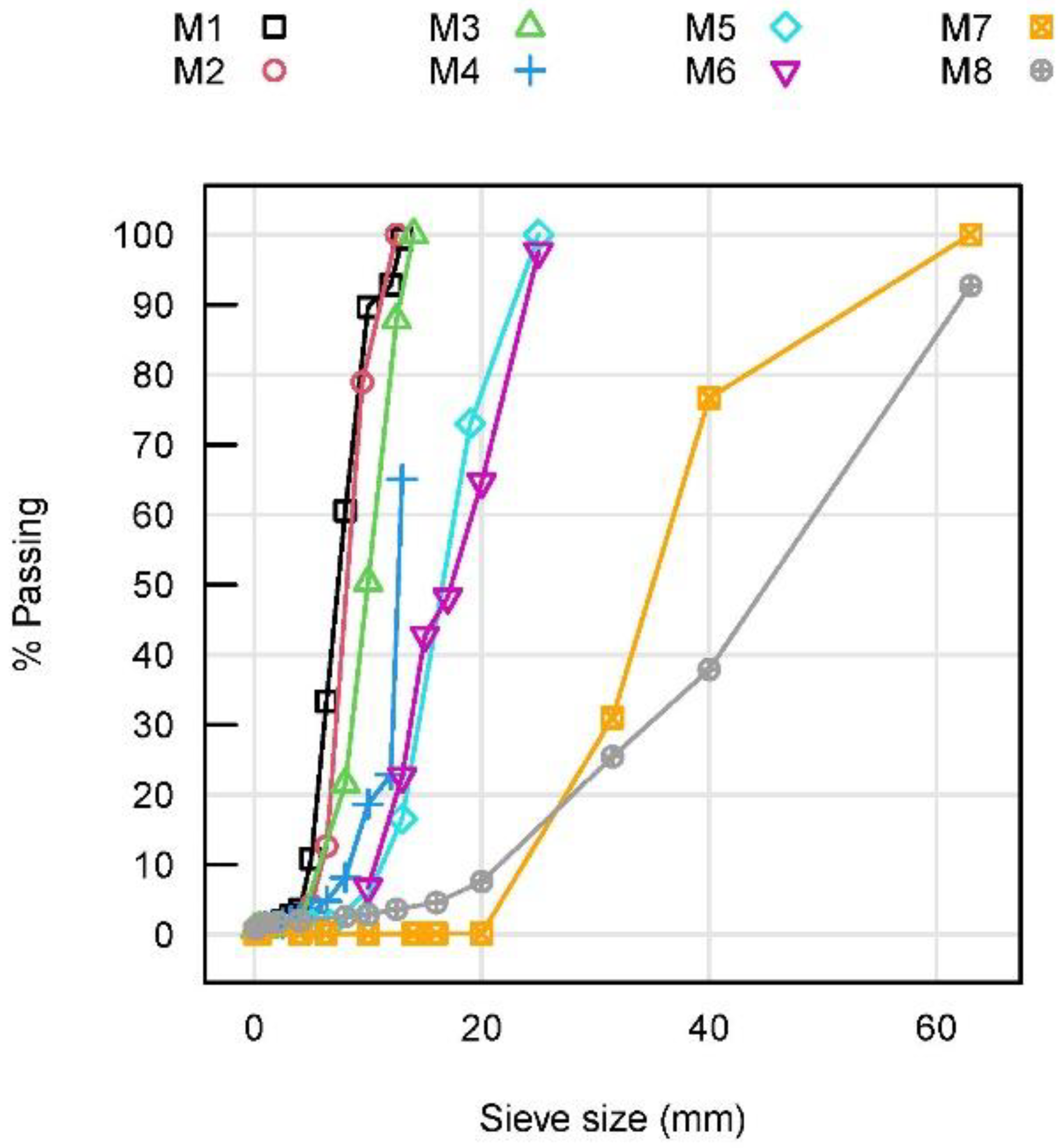
| Variable | M1 | M2 | M3 | M4 | M5 | M6 | M7 | M8 |
| D10 particle size [mm] | 4.89 | 5.97 | 5.72 | 8.36 | 11.11 | 10.62 | 23.68 | 21.58 |
| D50 particle size [mm] | 7.36 | 8.20 | 9.98 | 12.64 | 16.49 | 17.33 | 35.04 | 45.09 |
| Coefficient of uniformity (Cu) | 1.63 | 1.46 | 1.87 | 1.54 | 1.58 | 1.80 | 1.56 | 2.28 |
| Specific gravity (G) | NA | NA | 2.60 | NA | NA | NA | 2.50 | 2.60 |
| Dry unit weight (γd) [kN·m−3] | NA | NA | 14.7 | 16.1 | NA | 15.7 | 14.5 | 15.0 |
| Saturated unit weight (γd) [kN·m−3] | NA | NA | 18.9 | 19.9 | NA | 19.7 | 18.5 | 19.0 |
| Porosity (n) [%] | NA | NA | 42.6 | 39.3 | NA | 40.8 | 41.2 | 41.0 |
| Void ratio (e) [%] | NA | NA | 73.5 | 64.7 | NA | 68.9 | 69.5 | 66.0 |
| Angle of repose (φrepose) [degrees] | NA | NA | NA | 36.9 | NA | NA | 40.4 | 42.8 |
| Resistance law term a [s·m−1] | NA | NA | 1.44 | 2.71 | NA | 1.53 | 0.82 | 0.65 |
| Resistance law term b [s2·m−2] | NA | NA | 144.77 | 65.35 | NA | 84.66 | 52.82 | 16.96 |
| ‘Prototype’ Tests | ‘Small-Scale’ Models | |||||
|---|---|---|---|---|---|---|
| Test | Test | |||||
| 108 | 1.5 | 0.032749 | 109 | 1.5 | 0.005125 | 0.033558 |
| 110 | 2.5 | 0.042304 | 111 | 2.5 | 0.006618 | 0.043334 |
| 112 | 3.5 | 0.042505 | 130 | 3.5 | 0.006313 | 0.041337 |
Publisher’s Note: MDPI stays neutral with regard to jurisdictional claims in published maps and institutional affiliations. |
© 2022 by the authors. Licensee MDPI, Basel, Switzerland. This article is an open access article distributed under the terms and conditions of the Creative Commons Attribution (CC BY) license (https://creativecommons.org/licenses/by/4.0/).
Share and Cite
Monteiro-Alves, R.; Toledo, M.Á.; Moran, R.; Balairón, L. Failure of the Downstream Shoulder of Rockfill Dams Due to Overtopping or Throughflow. Water 2022, 14, 1624. https://doi.org/10.3390/w14101624
Monteiro-Alves R, Toledo MÁ, Moran R, Balairón L. Failure of the Downstream Shoulder of Rockfill Dams Due to Overtopping or Throughflow. Water. 2022; 14(10):1624. https://doi.org/10.3390/w14101624
Chicago/Turabian StyleMonteiro-Alves, Ricardo, Miguel Á. Toledo, Rafael Moran, and Luis Balairón. 2022. "Failure of the Downstream Shoulder of Rockfill Dams Due to Overtopping or Throughflow" Water 14, no. 10: 1624. https://doi.org/10.3390/w14101624
APA StyleMonteiro-Alves, R., Toledo, M. Á., Moran, R., & Balairón, L. (2022). Failure of the Downstream Shoulder of Rockfill Dams Due to Overtopping or Throughflow. Water, 14(10), 1624. https://doi.org/10.3390/w14101624