Using Stable Isotopes to Assess Groundwater Recharge and Solute Transport in a Density-Driven Flow-Dominated Lake–Aquifer System

Abstract

Saline lakes are mostly located in endorheic basins in arid and semi-arid regions, where the excess of evaporation over precipitation promotes the accumulation of salts on the surface. As the salinity of these lakes increases, their mass balance changes, and biogeochemical processes may be intensified. In that sense, Pétrola Lake (SE Spain) is a terminal lake located in an endorheic basin with elevated anthropic pressure, mainly derived from agricultural inputs and wastewater discharge. The goal of this study was to evaluate the interaction between groundwater and saline water from Pétrola Lake to improve our knowledge of groundwater recharge processes by density-driven flow (DDF) in terminal lakes. A combination of hydrochemical (chloride concentration) and stable isotope (δ¹⁸O_H2O and δ²H_H2O) data were used. In order to test the conceptual model, a simple numerical experiment was performed using a one-dimensional column that represents the relationship between the lake and the aquifer incorporating the variable density coupling control in solute migration. The isotopic composition of 190 groundwater and surface water samples collected between September 2008 and July 2015 provides a regression line (δ²H_H2O = 5.0·δ¹⁸O_H2O − 14.3‰, R² = 0.95) consistent with dominant evaporation processes in the lake. The DDF towards the underlying aquifer showed a strong influence on the mixing processes between the groundwater and surface water. Nevertheless, groundwater chemistry at different depths beneath the lake remains almost constant over time, suggesting an equilibrium between DDF and regional groundwater flow (RGF). Modelling isotope changes allowed inferring the temporal pattern of saline water recharge, coinciding with the summer season when water loss through evaporation is most significant. Consequently, the transport of solutes suitable for chemical reactions is then feasible to deeper zones of the aquifer.

1. Introduction

According to global estimates, the volume of inland saline waters in the world is around 85,000 km³ [1]. Saline lakes are common features of arid and semi-arid regions, where the excess of evaporation over precipitation results in the accumulation of salts at the land surface [2]. Therefore, they have a significant influence on the underlying groundwater affecting the hydrochemical evolution at the basin scale. Frequently, saline lakes are terminal discharge lakes representing the end-points of regional groundwater flow (RGF) as well as perimeter recharge areas. These terminal lakes may also be responsible for a significant amount of recharge from evaporated water, increasing the salinity of the shallow groundwater [3,4,5,6,7,8]. Groundwater recharge is produced by the wedged shape of a high-salinity zone [9]. Such high-salinity zones can be expanded laterally and vertically, being controlled partially by the groundwater inflow [10]. These systems can exert an important role in the natural attenuation of pollutants when organic matter is available [11] due to the transport of solutes by the density-driven flow (DDF). As a result, freshwater–saltwater interfaces (FSI) are hotspots for nutrient recycling in saline lakes [12,13]. Nevertheless, the exchange between lake water and groundwater is not always well-understood, and thus, the solute balance is difficult to quantify [14,15]. In this sense, the stable isotopes of the water molecule (δ¹⁸O_H2O and δ²H_H2O) have been widely used as tracers to provide information about the hydrogeological processes in saline lakes including precipitation, evaporation, groundwater recharge, and the mixing of waters, among others [16,17,18,19].

In this paper, the Pétrola endorheic basin was used as a study area using the combined approach of hydrochemical data, stable isotopes, and groundwater modelling. Pétrola Lake, the discharge point of the endorheic basin, is a terminal lake located in the La Mancha region (Albacete Province, SE Spain), which is one of the main areas of distribution of saline lakes in the Iberian Peninsula [20]. The anthropogenic pressure over this saline wetland alters the ecosystem functioning by modifying the mass balance and the intensity of biogeochemical processes [12]. Therefore, this study aims to (i) identify the source of the groundwater recharge in the Pétrola Basin; and (ii) determine the geochemical and hydrodynamic circumstances leading to the exchange of solutes between groundwater and surface water. This study provides new insights into the complexities of using stable isotopes of water to trace hydrogeological processes in highly saline systems.

2. Materials and Methods

2.1. Study Area

Pétrola Basin is an endorheic system located in southeastern Spain, in a semi-arid area (Figure 1). The endorheic basin of Pétrola (extends over 43 km²) is formed by an unconfined detrital aquifer (sands and clays) on which lies the saline lake. The aquifer is composed mostly of terrestrial and carbonate units whose thickness can exceed 60 m, ranging in age from Barremian to Albian. As shown in [21], the hydraulic conductivity of these materials varies (0.01–60 m/day), with a high storage capacity (30%). The impermeable bottom is formed by the clayey materials of the base of the Cretaceous.

The groundwater flow is radial and centripetal from the recharge areas (system boundaries) to the Pétrola Lake that occupies the terminal discharge zone of the basin. Horizontal head gradients are between 10⁻³ and 10⁻². Vertical head gradients across the area are generally downward except in the immediate vicinity of the lake where they are upward. Pétrola Lake has an extension of about 1.76 km², and a depth that does not exceed 2 m (Confederación Hidrográfica del Segura, unpublished data). As pointed out, surface runoff is not of great importance since the courses are irregular and even disappear in relation to lithology [22]. However, the drainage network flows into the lake and can function intensively in the event of significant rainfall. Under natural conditions, seasonal fluctuations in water volume are largely found as a response to climatic events.

The study area is characterised by irregular rainfall periods, alternating long episodes of drought and torrential precipitations. Maximum water volume stored in the lake is found in early spring (about 1.5 hm³ in 1.6 km²) when abundant precipitation and low evaporation rates occur. However, minimum volume or complete dryness can be observed at the end of summer, associated with few precipitation events and maximum evaporation rates [23], which causes an increase in the concentration of salts in the lake. In fact, there are important density contrasts between the hypersaline water of the lake (up to 1.3 g/cm³) and freshwater from the aquifer (around 1 g/cm³). A buoyancy DDF from the lake towards the underlying aquifer is found in the saline lake–aquifer interface because of the instability of the saline boundary layer [12,13,21].

2.2. Field Survey

Sampling locations are shown in Figure 1. A total of 190 water samples from 27 control points (springs, surface water including streams and lakes, and agricultural wells) were collected in two distinct periods. An initial field campaign was carried out from September 2008 to October 2011. In order to acquire more information about the system, a second field survey was performed from March 2013 to July 2015. Additionally, four PVC piezometers at different depths (GW-12 at 12.1 mbgs, GW-26 at 25.8 mbgs, GW-34 at 34.1 mbgs, and GW-38 at 37.9 mbgs) (mbgs: meters below ground surface) were installed during 2008 near the lake border, as described by [18,21]. The study area has been divided into three groups: Zone 1, Zone 2, and Zone 3 (Figure 1). Zone 1 matched with the recharge area, including the following control points: 2535, 2548, 2553, 2564, 2579, 2581, 2582, 2621, and 2645. Zone 2 comprised control points located near the lake, following the groundwater flow direction from Zone 1 to the discharge zone. Control points included in Zone 2 were: 2554, 2571, 2575, 2599, 2602, 2640, 2641, and 2642. Zone 3 represented the zone of density-driven groundwater flow located under the lake (piezometers) and lake surface waters. This area can be subdivided into smaller subzones according to different anthropogenic pressures around the lake. Zone 3A referred to control point 2643 and was placed in the southern part of the lake, where wastewaters reached the lake. Isolated areas for salt exploitation were embraced by Zone 3B and included control point 2635 and piezometers (GW-12, GW-26, GW-34 and GW-38). Finally, Zone 3C comprised control points 2648, 2649, 2651, and 2652, which were affected by the irrigation return flows from the adjacent farming areas.

In piezometers GW-12, GW-26, and GW-34, groundwater levels were measured at 24 h intervals between February 2010 and October 2011 (n = 609 daily measurements) employing a ceramic CTD-Diver stand-alone sensor. Groundwater level measurements in piezometer GW-38 were omitted since it is a flowing well. Precipitation and humidity data for the study period were obtained from meteorological station AB07 (Ministry of Agriculture and Fisheries, Food and Environment of Spain) located about 16 km from Pétrola Lake, in Pozo Cañada (Albacete province, SE Spain).

2.3. Physical–Chemical and Isotopic Analyses

Groundwater temperature (T), pH, redox potential (Eh), electrical conductivity (EC), and dissolved oxygen (DO) were measured in situ with portable electrodes. In springs, streams, and well control points, measurements were performed directly in the water flow. Measurements in the piezometers were made using a flow-through chamber to minimize the effect of air exchange. Water samples were filtered with a 0.45 µm nylon Millipore^® filter and stored at 4 °C in darkness prior to further analysis and following the official standard methods [24]. For samples collected between September 2008 and October 2011, bicarbonate (HCO₃⁻), sulfate (SO₄²⁻), and chloride (Cl⁻) concentrations were measured by ion chromatography (DX120, Vertex). In those samples, main cations (Na⁺, K⁺, Ca²⁺ and Mg²⁺) were measured in an atomic absorption spectrophotometer equipped with an air-acetylene burner. For samples collected during the field campaign in 2013, concentrations of Cl⁻ and SO₄²⁻ were acquired by capillary electrophoresis (CE) using a Waters Quanta 4000 system coupled with a negative power supply and an indirect UV detection system, as described by [25]. Alkalinity measurements were performed by acid–base titration in the laboratory of Biotechnology and Natural Resources (University of Castilla-La Mancha). Aqueous concentrations of K⁺, Na⁺, Ca²⁺, and Mg²⁺ were measured by combining CE and ICP-AES for those samples. Analyses of CE and ICP-AES were attained from the research services at the National Museum of Natural History (Madrid, Spain). Density was estimated using AquaChem software [26].

¹⁸O/¹⁶O ratios from H₂O were measured by the CO₂ equilibration method. δ¹⁸O_H2O from samples collected between April 2008 and October 2010 were measured using a Multiflow device coupled online to a continuous flow Isoprime Mass Spectrometer at the Stable Isotopes Laboratory at the University of Salamanca (LIE-US). For those samples, δ²H_H2O values were obtained by measuring ²H in the reduction of Cr with an elemental analyzer (EuroVector) coupled to a continuous flow mass spectrometer (Isoprime Mass Spectrometer) at LIE-US. δ¹⁸O_H2O and δ²H_H2O in samples collected between April 2013 and July 2015 were measured by DI-IRMS on a Finnigan Mat Delta at the Centres Cientific Tècnis of Universitat de Barcelona (CCiT-UB). Results were expressed in δ‰ values relative to Vienna Standard Mean Ocean Water (VSMOW) for δ¹⁸O_H2O and δ²H_H2O. For both δ¹⁸O_H2O and δ²H_H2O calibration, four international standards (USGS 46, USGS 47, USGS 48, and USGS 50) and one internal laboratory standard were used as reference materials and then normalised against the VSMOW scale. Analytical reproducibility by repeated analysis of both international and internal reference samples of known isotopic compositions was determined to be about ±0.3‰ and ±1‰, respectively for δ¹⁸O_H2O and δ²H_H2O in waters.

2.4. Methods for Evaporation Modelling

By using δ¹⁸O_H2O and δ²H_H2O results in the studied area, a Local Meteoric Water Line (LMWL) was calculated for Pétrola Basin using a linear regression model. The Madrid and Murcia stations can be considered as an approximation for the local meteoric water lines, since measured isotope data from Zones 1 and 2 were suited to Madrid Meteoric Water Line (MaMWL) from Madrid-Retiro station (655 m above sea level, masl), and Murcia Meteoric Water Line (MuMWL) at 62 masl. Both water lines were calculated using data from the International Atomic Energy Agency (IAEA) [27] from 1970 to 2006, only considering values related to dates with precipitation over 20 mm (n = 109) [28]. In order to check the reliability of the calculated slope, the isotopic relationships derived by [29] were used to mathematically predict the slope of the evaporation line for the water body of the Pétrola lake-aquifer system. As described by [30], the required variables were (i) the initial isotopic composition of water; (ii) temperature during evaporation; iii) relative humidity of the air mass; and iv) the isotopic composition of water vapour (δ¹⁸O_v, δ²H_v).

The intersection point between the MaMWL and the LMWL (δ¹⁸O_H2O = −7.8‰ and δ²H_H2O = −53.8‰) was set as the initial isotopic composition of water. A temperature of 20.7 °C was considered for modelling purposes during evaporation since this value was the average maximum temperature for the period 1981–2010. The value considered as initial relative humidity was 0.68 since it was the mean annual relative humidity in the Pozo Cañada SIAR station. To estimate the value of δ¹⁸O_v and δ²H_v, the oxygen and hydrogen liquid water–vapour fractionation factors (α_O and α_H) were calculated following the work of [31]:

ln α_O = 1137/T² − 0.4156/T − 0.00207,

(1)

ln α_H = 24844/T² − 76.248/T + 0.05261,

(2)

where T is expressed in Kelvin. Using a temperature of 20.7 °C (293.85 K), the fractionation factors obtained were α_O = 1.0097 and α_H = 1.0842. Then, isotopic compositions in equilibrium between liquid water and water vapour (δ¹⁸O_veq and δ²H_veq) were obtained by using the calculated fractionation factors (α_O and α_H) in the Equations of [32]:

α_O = (1 + 10⁻³ · δ¹⁸O_i)/(1 + 10⁻³ · δ¹⁸O_veq),

(3)

α_H = (1 + 10⁻³ · δ²H_i)/(1 + 10⁻³ · δ²H_veq),

(4)

where δ¹⁸O_i and δ²H_i were the isotopic compositions at the intersection point, which provided values of δ¹⁸O_veq = –17.4‰ and δ²H_veq = –127.3‰. Subsequently, Equations (5) and (6) from [33] were used to determine the actual water vapour composition (δ¹⁸O_v and δ²H_v):

δ¹⁸O_v = (δ¹⁸O_veq + 1.4)/0.9,

(5)

δ²H_v = δ²H_veq + 2,

(6)

Consequently, the obtained values for δ¹⁸O_v and δ²H_v were –17.7‰ and –125.3‰, respectively. To consider short-term variations, δ¹⁸O_v and δ²H_v should be directly measured. Nevertheless, the calculated values are adequate when no direct measurements are available [7]. In order to evaluate the loss of water in the lake by means of stable isotope data, the isotopic changes during evaporation of surface water have been modelled following the modified equations of [29] (Equations (7)–(9)). Those equations constrain the theoretical evolution in the isotopic composition of the residual lake water (δ¹⁸O_L and δ²H_L) as a function of the fraction of lake water that has been lost to evaporation.

Δ_L = (δ_i − A/B)f^B + A/B,

(7)

For calculation purposes, δ_i (δ¹⁸O_i and δ²H_i) has been considered as the initial isotopic composition at the intersection point (−7.8‰ and −53.8‰, respectively), f was the fraction of lake water that has been evaporated. Constants A and B were defined by:

$$\mathrm{A}=\left(\frac{\mathrm{h}}{{\mathrm{aH}}_2{\mathrm{O}}_{\mathrm{L}}}{\mathsf{\delta }\mathrm{v}}_{\mathrm{i}}+{\mathsf{\Delta }\mathsf{\epsilon }}_{\mathrm{i}}+\frac{{\mathsf{\epsilon }}_{\mathrm{i}}}{{\mathsf{\alpha }}_{\mathrm{i}}}\right)/\left(1-\frac{\mathrm{h}}{{\mathrm{aH}}_2{\mathrm{O}}_{\mathrm{L}}}+\frac{{\mathsf{\Delta }\mathsf{\epsilon }}_{\mathrm{i}}}{1000}\right),$$

(8)

$$\mathrm{B}=\left(\frac{\mathrm{h}}{{\mathrm{aH}}_2{\mathrm{O}}_{\mathrm{L}}}-\frac{{\mathsf{\Delta }\mathsf{\epsilon }}_{\mathrm{i}}}{1000}-\frac{{\mathsf{\epsilon }}_{\mathrm{i}}}{{1000\mathsf{\alpha }}_{\mathrm{i}}}\right)/\left(1-\frac{\mathrm{h}}{{\mathrm{aH}}_2{\mathrm{O}}_{\mathrm{L}}}+\frac{{\mathsf{\Delta }\mathsf{\epsilon }}_{\mathrm{i}}}{1000}\right),$$

(9)

where h was humidity and aH₂O_L was the activity of the water in the lake calculated from Cl⁻ concentration in mmol/kg (aH₂O_L = 1 – 6·10⁻⁹·Cl₂ – 2·10⁻⁵·Cl; from [34]). Δv_i was the obtained values for δ¹⁸O_v and δ²H_v of the water vapour (–17.7‰ and –125.3‰, respectively), α_i values were the equilibrium isotopic fractionation factor calculated above, ε_i was the isotopic enrichment (ε = 1000 · (α_i – 1)), and Δε was the kinetic enrichment factor. Δε value for O was 14.5 (1 – h/aH₂O_L), whereas Δε value for H was 12.5 (1-h/ aH₂O_L) [29]. In the model, neither inputs nor outputs to the water body other than loss of water due to evaporation are assumed. Halite precipitation was also considered for modelling purposes at a Cl⁻ concentration of 4500 mmol/kg, and further evaporation maintains halite saturation [7].

3. Results

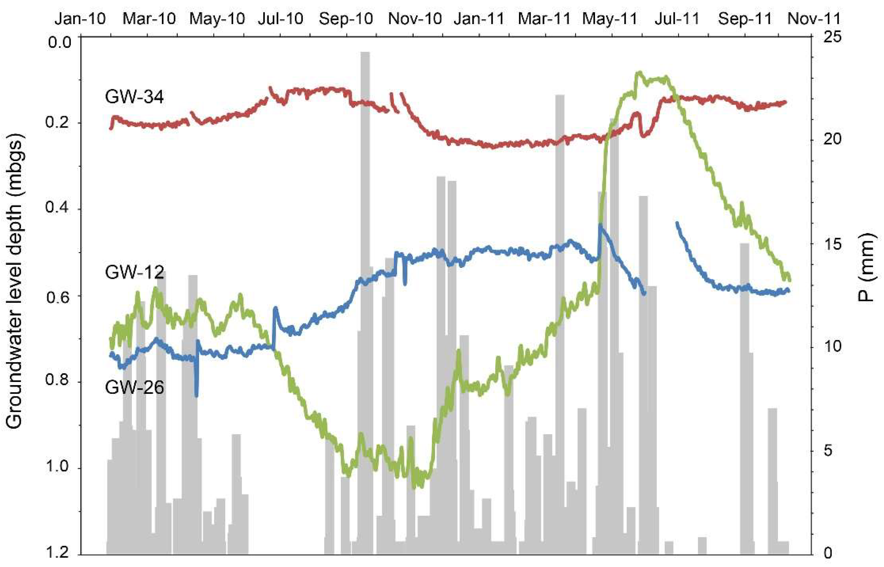
3.1. Groundwater-Level Evolution

The groundwater level was measured in piezometers GW-12, GW-26, and GW-34. The groundwater-level evolution was affected by precipitation events and regional groundwater potential (Figure 2). The groundwater level in GW-12 was generally influenced by the water level variations in the lake, mainly related to the local precipitation pattern. In the GW-12 piezometer, a noticeable decrease in groundwater levels was found from the end of June 2010 to mid-November 2010, coinciding with the end of the dry months. Further groundwater-level increases concurred with a period of intense and regular precipitation. The groundwater evolution in GW-34 largely reflected variations in the regional groundwater potential in contrast to the GW-12 piezometer. From February 2010 to July 2010, the groundwater potential showed a subtle increase. From July 2010 to mid-November 2010, the groundwater levels recorded showed a decreasing trend but the values did not show the variations observed in GW-12 for the same period. Then, the groundwater level in GW-34 suffered a slight decrease and remained constant until June 2011, contrary to the dramatic increase observed in GW-12 for the same period. The water level in GW-26 remained nearly constant from February 2010 to July 2010 and then increased until May 2011. Afterwards, the groundwater level showed a tendency to drop. An accidental malfunction of the diver installed in GW-26 could explain the observed discontinuities in the groundwater levels recorded during the period May–July 2011.

3.2. Physical–Chemical Results

The chemical and isotopic results are summarised in

Table 1. Mean values of the chemical and isotopic analyses in water samples. EC: electrical conductivity (µS/cm). TDS: total dissolved solids (g/L). Eh: redox potential (mV). DO: dissolved oxygen (mg/L). T: temperature (°C). ρ: density (g/cm³). Cl⁻ expressed in mmol/kg. Isotope values expressed in ‰. Nd: not determined.

Sample Point	Group	pH	EC	TDS	Eh	DO	T	ρ	Cl−	δ18OH2O	δ2HH2O
2535	Zone 1	7.5	1174	0.50	nd	1.8	nd	1.00	1.65	−6.5	−48.9
2548	Zone 1	nd	nd	nd	nd	nd	nd	nd	nd	−6.6	−50.4
2553	Zone 1	7.3	689	0.20	nd	7.2	nd	1.00	1.52	−7.6	−51.6
2564	Zone 1	7.8 ± 0.1	1492 ± 59	0.69	314 ± 129	5.6 ± 1.9	16.3 ± 3.5	1.00 ± 0.00	3.05 ± 0.23	−6.9 ± 0.8	−47.4 ± 2.2
2579	Zone 1	7.4 ± 0.1	1048 ± 47	0.42	194 ± 4	2.3 ± 1.6	25.0	1.00 ± 0.00	1.59 ± 0.30	−6.7 ± 0.9	−52.3 ± 0.5
2581	Zone 1	7.3 ± 0.1	1253 ± 15	0.54	328 ± 139	3.4 ± 1.1	18.0 ± 4.0	1.00 ± 0.00	1.19 ± 0.20	−6.7 ± 0.6	−45.7 ± 3.6
2582	Zone 1	7.3	1755	0.84	nd	0.9	nd	1.00	2.64	−6.8	−49.5
2621	Zone 1	7.4	1008	0.40	nd	2.3	nd	1.00	1.08	−3.1	−55.5
2645	Zone 1	nd	nd	nd	nd	nd	nd	nd	nd	−6.4	−51.9
2554	Zone 2	7.8 ± 0.2	1546 ± 226	0.72	346 ± 115	5.4 ± 1.8	14.9 ± 4.1	1.00 ± 0.00	2.75 ± 0.32	−6.2 ± 0.5	−46.5 ± 2.4
2571	Zone 2	7.9 ± 0.2	1638 ± 227	0.77	277 ± 145	5.3 ± 2.4	14.0 ± 5.4	1.00 ± 0.00	4.16 ± 1.73	−6.1 ± 1.3	−46.4 ± 4.9
2575	Zone 2	7.9 ± 0.3	1458 ± 218	0.67	91 ± 199	3.9 ± 3.6	16.7 ± 5.7	1.00 ± 0.00	5.40 ± 1.05	−6.3 ± 1.1	−46.5 ± 1.9
2599	Zone 2	7.9	1753	0.84	nd	1.7	nd	1.00	6.00	−5.8	−48.2
2602	Zone 2	8.2 ± 0.2	2426 ± 540	1.25	264 ± 113	6.7 ± 2.3	14.7 ± 4.1	1.00 ± 0.00	7.58 ± 0.97	−5.6 ± 1.4	−44.4 ± 9.2
2640	Zone 2	8.3 ± 0.1	1858 ± 408	0.91	300 ± 126	7.8 ± 1.6	13.7 ± 5.2	1.00 ± 0.00	4.25 ± 1.78	−6.0 ± 1.7	−44.4 ± 9.4
2641	Zone 2	8.0 ± 0.2	1349 ± 131	0.60	315 ± 94	7.1 ± 2.8	15.7 ± 4.5	1.00 ± 0.00	4.27 ± 0.63	−6.1 ± 1.6	−46.4 ± 9.1
2642	Zone 2	8.1 ± 0.1	2241 ± 458	1.14	327 ± 98	6.8 ± 2.2	12.9 ± 6.0	1.00 ± 0.00	4.10 ± 0.73	−5.8 ± 1.7	−44.6 ± 9.2
2643	Zone 3A	9.0 ± 0.5	38,929 ± 21,056	23.15 ± 12.4	233 ± 160	8.9 ± 2.0	14.6 ± 6.5	1.03 ± 0.02	309 ± 156	+2.9 ± 5.1	+5.9 ± 25.9
2635	Zone 3B	8.5 ± 0.4	37,027 ± 28,935	22.01 ± 17.2	266 ± 108	6.8 ± 3.3	16.8 ± 6.9	1.05 ± 0.07	534 ± 891	+1.6 ± 2.9	−5.5 ± 16.0
GW-12	Zone 3B	7.0 ± 0.0	89,043 ± 6803	53.22 ± 3.9	22 ± 143	0.6 ± 1.4	18.2 ± 1.6	1.09 ± 0.01	1157 ± 193	−2.7 ± 1.3	−22.1 ± 4.4
GW-26	Zone 3B	6.9 ± 0.1	56,543 ± 11,375	33.72 ± 6.6	120 ± 173	0.2 ± 0.2	17.9 ± 2.6	1.05 ± 0.02	571 ± 202	−4.7 ± 1.0	−38.1 ± 1.8
GW-34	Zone 3B	7.0 ± 0.1	10,263 ± 7286	5.95 ± 4.2	90 ± 100	0.4 ± 0.2	18.7 ± 3.3	1.01 ± 0.00	94.0 ± 61.0	−5.9 ± 1.5	−45.4 ± 3.9
GW-38	Zone 3B	7.3 ± 0.5	2423 ± 574	1.24 ± 0.1	153 ± 95	1.0 ± 1.2	18.7 ± 3.1	1.00 ± 0.00	6.51 ± 2.06	−7.1 ± 0.9	−49.5 ± 1.8
2648	Zone 3C	8.6 ± 0.2	35,425 ± 15,464	21.05 ± 9.1	170 ± 179	8.2 ± 5.5	14.4 ± 5.9	1.04 ± 0.02	335 ± 199	+3.5 ± 4.1	+3.9 ± 17.5
2649	Zone 3C	8.7 ± 0.1	45,350 ± 18,031	27.00 ± 10.6	−45 ± 258	4.5 ± 6.1	17.5 ± 6.2	1.05 ± 0.02	439 ± 205	+1.6 ± 11.6	−9.0 ± 53.7
2651	Zone 3C	8.8 ± 0.1	51,150 ± 29,628	30.48 ± 17.6	143 ± 11	6.7 ± 3.4	20.1 ± 12.0	1.05 ± 0.02	441 ± 172	+4.6 ± 6.9	+8.2 ± 31.2
2652	Zone 3C	8.7 ± 0.1	46,850 ± 21,567	27.90 ± 12.7	150 ± 15	5.3 ± 4.1	18.2 ± 4.5	1.07 ± 0.00	635 ± 48	+4.1 ± 9.2	+3.2 ± 42.9

. The TDS has been calculated from the EC values. The chloride concentrations as mmol/kg were calculated from the original concentration (in mg/L) and density values. The complete analytical results are presented in the Supplementary Materials (Table S1). In Zone 1, the groundwater type varied between Mg-Ca-HCO₃ and Mg-Ca-SO₄ hydrofacies (7 control points, n = 16) (Figure 3). Those water samples had the lowest EC values, varying between 689 μS/cm (control point 2553) and 1755 μS/cm (control point 2582). The density values were constant, with a value of 1.00 g/cm³ (n = 16). The chloride concentrations oscillated from 0.96 mmol/kg in control point 2581 to 3.32 mg/L in control point 2564, with an average value of 2.10 mmol/kg (n = 16). The values of δ¹⁸O_H2O in Zone 1 varied from −8.0‰ (in 2579) to −3.1‰ (in 2621), with a mean value of −6.6‰ (n = 22). The δ²H_H2O data varied between −55.5‰ (in 2621) and −39.8‰ (in 2581), showing a mean value of −49.0‰ (n = 22). The water samples from Zone 2 showed hydrofacies similar to those in Zone 1, varying between Mg-Ca-SO₄-HCO₃ and Na-Ca-HCO₃-Cl (8 control points, n = 90) (Figure 3). Zone 2 provided higher EC values than the samples from Zone 1, which varied from 1060 μS/cm in control point 2640 to 3200 μS/cm in control point 2602. The density values were also stable (1.00 g/cm³, n = 90). The chloride concentration varied between 2.38 mmol/kg (in 2554) and 10.2 mmol/kg (in 2640), with a mean value of 4.46 mmol/kg (n = 90). The δ¹⁸O_H2O values ranged from −8.7‰ (in 2640) to −0.7‰ (also found in 2640), with an average value of −6.0‰ (n = 93), whereas the values of δ²H_H2O ranged from −52.4‰ (in 2641) to −12.8‰ (in 2640), with an average value of −45.7‰ (n = 94).

Concerning the water samples from Zone 3, excluding the groundwater from the piezometers, the EC values ranged from 14,600 μS/cm (May 2013, control point 2635) to 123,000 μS/cm (November 2010, control point 2635). The density values ranged from 1.01 g/cm³ (samples collected between March and June 2013 in control point 2635) to 1.29 g/cm³ (October 2010, control point 2635). The chloride concentrations ranged from 92.7 mmol/kg (April 2013, control point 2635) to 3751 mmol/kg (October 2010, control point 2635), with a mean value of 478.6 mmol/kg (n = 46). Hydrofacies showed a Mg-Na-SO₄-Cl composition (6 control points, n = 46) (Figure 3). The δ¹⁸O_H2O isotope compositions varied between −6.7‰ (April 2015, control point 2649) and +11.0‰ (July 2015, control point 2643), with an average value of +2.2‰ (n = 46). Values of δ²H_H2O varied between −48.2‰ (April 2015, control point 2643) and +35.4‰ (July 2015, control point 2635), with a mean value of −2.2‰ (n = 46).

With regard to the piezometer data, hydrofacies varied between Mg-Ca-SO₄-HCO₃ (GW-38) and Mg-Na-SO₄-Cl (GW-12) (4 control points, n = 28) (Figure 3). The electrical conductivity ranged from 1170 μS/cm in the deepest-screened piezometer (GW-38) to 98,600 μS/cm in the shallowest one (GW-12). The values of the density varied between 1.00 g/cm³ (GW-38) and 1.10 (GW-12). The chloride concentrations ranged from 1304 mmol/kg (in GW-38) to 3.80 mmol/kg (in GW-12). The δ¹⁸O_H2O data varied between −8.8‰ (in GW-38) and −1.4‰ (in GW-12), with a mean value of −5.2‰ (n = 28), whereas the δ²H_H2O data ranged from −52.4‰ (in GW-38) to −14.5‰ (in GW-12), showing an average value of −39.7‰ (n = 23).

3.3. Evaporation Modelling

The isotopic composition of water samples was displayed in a δ¹⁸O-δ²H diagram (Figure 4). From the δ¹⁸O_H2O and δ²H_H2O results in the studied area, the LMWL was calculated: δ²H_H2O = (5.0 ± 0.1)·δ¹⁸O − (14.3 ± 0.5)‰ (R² = 0.95). Those results were compared with the MaMWL (δ²H_H2O = 7.5·δ¹⁸O + 4.6‰; R² = 0.90) and the MuMWL (δ²H_H2O = 6.8·δ¹⁸O + 2.4‰; R² = 0.88). The obtained regression line for the δ¹⁸O_H2O and δ²H_H2O results (δ²H_H2O = 5.0·δ¹⁸O − 14.3‰) showed a slope (5.0) consistent with the evaporation processes. The slope of the evaporation line is dependent upon the ambient humidity, decreasing from near 8.0 (100% humidity) to 3.7 (0% humidity) [29]. The slope of the calculated evaporation line (5.0) suggested that evaporation took place at humidity values of about 69.8%. The humidity values in the Pozo Cañada SIAR station during the dry period varied between 44% and 73% (±1σ) (mean annual relative humidity of about 68%).

The results indicated that δ¹⁸O_H2O was observed in surface water areas due to the evaporation of rainwater with similar isotope compositions to the average precipitation of Madrid. The model showed that most of the lake water samples collected during both field campaigns corresponded to evaporation trends at a humidity between 60% and 75%. Nevertheless, a group of lake water samples collected during July 2015 showed an evaporation trend at a lower humidity (around 55%). The model also showed that in the presence of high salt concentrations, the heavy isotope content of the residual brine would describe an increasing trend to a certain extent, and then the trend would reverse towards the depleted δ¹⁸O_H2O values. The relatively depleted δ¹⁸O_H2O values found at high salinities may complicate the interpretation of data. It was expected that the samples belonging to the dry seasons would show relatively high Cl⁻ concentrations and heavy isotopic values. This trend was detected for lake water samples collected during a field survey in 2013, with a weak positive correlation between δ¹⁸O_H2O and Cl⁻ concentrations (R² = 0.35, n = 37). Nevertheless, it was not observed in the more evaporated samples from the field survey in 2010. These results suggested that the use of isotope values is unadvisable for mixing calculations at high salinities.

4. Discussion

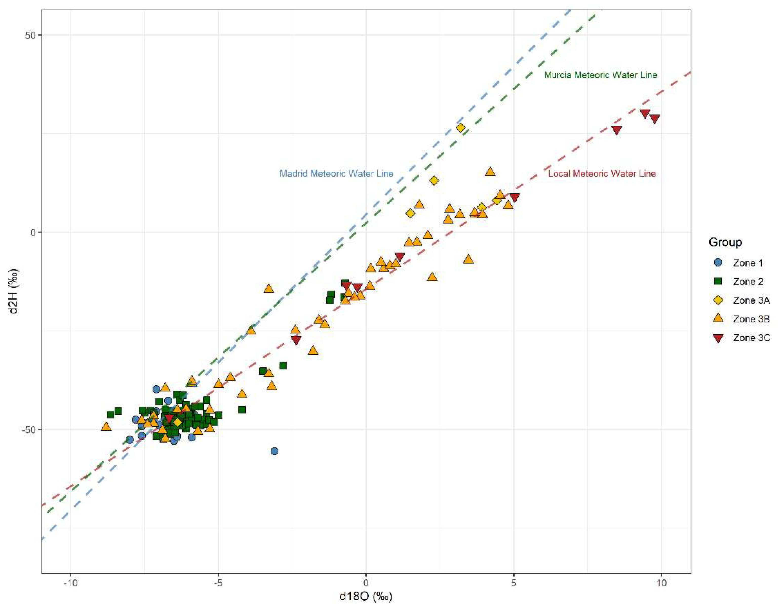
4.1. Source of Precipitation

The major sources of water vapour in Spain are the Mediterranean sea and the Atlantic Ocean [35]. Due to the location of the study area, both sources must be considered. The deuterium excess (d-value = δ²H_H2O − 8·δ¹⁸O from [36]) can be employed to recognize the potential sources of water vapour [37]. In the recharge area from Pétrola Basin (Zone 1), the mean d-value was +5.8‰ (n = 21). It was noted in Ref. [38] that the Atlantic origin precipitation was characterized by d-values up to +10‰. On the other hand, Mediterranean-derived precipitation provided higher d-values close to +27‰ due to the low relative humidity in the Mediterranean area, which is the main moisture provider during extreme events [39]. Due to its location, the Pétrola basin may have moisture inputs from the western Atlantic-dominated and eastern Mediterranean-dominated, domains of the Iberian Peninsula [40]. Our results suggested that the groundwater recharge in the Pétrola Basin was mainly produced by Atlantic-derived precipitation, relegating the Mediterranean precipitation to a secondary role. Our findings were consistent with those of [41]. They concluded that the most intense rain events in western Spain are generally related to humid air masses originating in the tropical Atlantic mostly during autumn and spring. The effects of the air masses produced over the Mediterranean can result in local noise during summer events, but it is commonly restricted to a short distance from the shoreline. It usually occurs in form of extreme precipitation events (>100 mm in a few hours) during September and October. This hypothesis was also supported by the highest d-values calculated in the Pétrola Basin. The highest d-values should be related to the eventual Mediterranean precipitation events. The maximum d-value (+17.0‰) in Zone 1 was observed in control point 2581 in October 2010. In Zone 2, the highest d-values were calculated for the samples collected during September 2013 (+22.9‰, control point 2640). Moreover, a d-value of +20.9‰ was calculated for a sample collected in October 2011 from piezometer GW-38.

4.2. Surface and Groundwater Interaction in the Vicinity of the Lake

Regional groundwater flow is radial and centripetal from the boundaries of the basin (recharge areas, i.e., Zone 1) to the lake, as observed in other saline-lake systems [42,43]. In Pétrola Lake, the surface water density reached values of up to 1.29 g/cm³ (October 2010, Table S1), whereas several groundwater samples showed density values of 1.00 g/cm³ in piezometers GW-38 and GW-34. As a result of such density differences, a DDF towards the underlying aquifer was produced defining the FSI. These interfaces are hot spots of nutrient turnover and pollutants removal [11,44,45] where the DDF is the main driver. Thus, wet–dry periods can modify both the surface water chemistry and biogeochemical processes by affecting the DDF dynamics. During the wet periods, the increase in precipitation (mainly rainfall) dilutes the surface water, whereas in dry periods surface water salinity increases due to evaporation [18].

The input of water from Pétrola Lake into the underlying aquifer was evidenced by the patterns of stable isotope and Cl⁻ concentrations. This was particularly apparent in the groundwater samples from the 2008 survey since it included samples collected at different depths below the lake. Chloride can be assumed as conservative, since maximum Cl⁻ concentrations (3751 mmol/kg measured in control point 2635, October 2010) was below the saturation of halite (4500 mmol/kg; [7]) and may have been related to the dissolution of salts precipitated in the lake during previous dry seasons. The samples collected at piezometers GW-38, GW-34, GW-26, and GW-12, indicated that the Cl⁻ concentration was stable over time, showing a decrease with depth throughout the sampling period. The Cl⁻ concentrations were higher in GW-12 than in the surface water for samples taken in February 2010, April 2010, and October 2011. These samples were collected during the wet periods due to precipitation events that produce the dilution of surface waters. The samples taken in July 2010, October 2010, and November 2010 showed higher Cl⁻ contents in the surface water than in the groundwater (GW-12). Our results were in line with the absence of precipitation events during the summer of 2010, which allowed evaporation processes to control the salt concentrations in the surface water [46].

In general, it seems that the chemical data were also reflected in the measured groundwater-level evolution (Figure 2). Between July 2010 and November 2010, the groundwater level in GW-12 decreased, whereas the groundwater level in GW-26 increased. It would imply that the amount of Cl⁻ from the regional groundwater reaching piezometer GW-12 should increase coinciding with the Cl⁻ increase due to the loss of water by evaporation. The response of the system was to increase the potentiometric level, as observed in GW-34 (Figure 2). On the other hand, the heaviest δ¹⁸O_H2O values in the piezometers were found from February to March 2010, coinciding with the lowest groundwater potential in GW-34, whereas the lightest ones were observed in July 2010 when the groundwater potential in GW-34 was higher. Consequently, the volume of water returning to the aquifer should decrease coupled with the increase in the water density. Therefore, the surface water level and salt content in the system should be at a steady state when the inputs (i.e., regional groundwater potential) were similar to the outputs (i.e., evaporation, recharge by DDF and mineral formation).

Stable isotope data also provided evidence for this hypothesis. At the end of the dry period in 2010 (samples from October and November), the minimum differences between the surface water and GW-12 in δ¹⁸O_H2O were found. Moreover, the δ²H_H2O values were lower in the surface water than in GW-12. Thus, evaporated water can be found at 12 mbgs. The recharge of water from the Pétrola Lake to the groundwater was evidenced by the enrichment of the ¹⁸O and ²H isotopes in the groundwater samples collected from the piezometers. Our results from modelling showed that the intersection point between the isotopic evolution of the surface water and the mixing line described by the piezometer samples represents the time at which the saline boundary layer is formed. Attending to our data, the largest influence of the RGF would take place mainly from July to November 2010, coinciding with the lowest groundwater water depth in GW-12 (Figure 2, densities of 1.24 g/cm³). According to this assumption, the GW-12 samples with a mean Cl⁻ concentration for the study period of about 1092 mM, would represent a mix of about 30% of the water from the RGF. This indicates that the RGF can be much larger than the DDF groundwater component of water in the system. It was also noticeable that the δ¹⁸O_H2O and δ²H_H2O values in the piezometers had much less variability than those values from the surface water. Thus, despite the important variations observed in the surface water (Cl⁻, δ¹⁸O_H2O and δ²H_H2O), the groundwater chemistry showed negligible variations suggesting an equilibrium between the DDF and RGF.

The results allowed us to infer that the formation of a saline boundary layer in the Pétrola lake–aquifer system is sensitive to both changes in the hydraulic gradient and the solute concentrations. It may imply changes in the transport rates of chemical species in the underlying aquifer, and thus in the rate of pollutant attenuation at the FSI [13]. As noted by [47], the influence of the differences in water density may be masked when the regional hydraulic gradient is high enough. Therefore, a reduced transport of reactants from the lake to the deeper parts of the aquifer will be expected during low lake water periods.

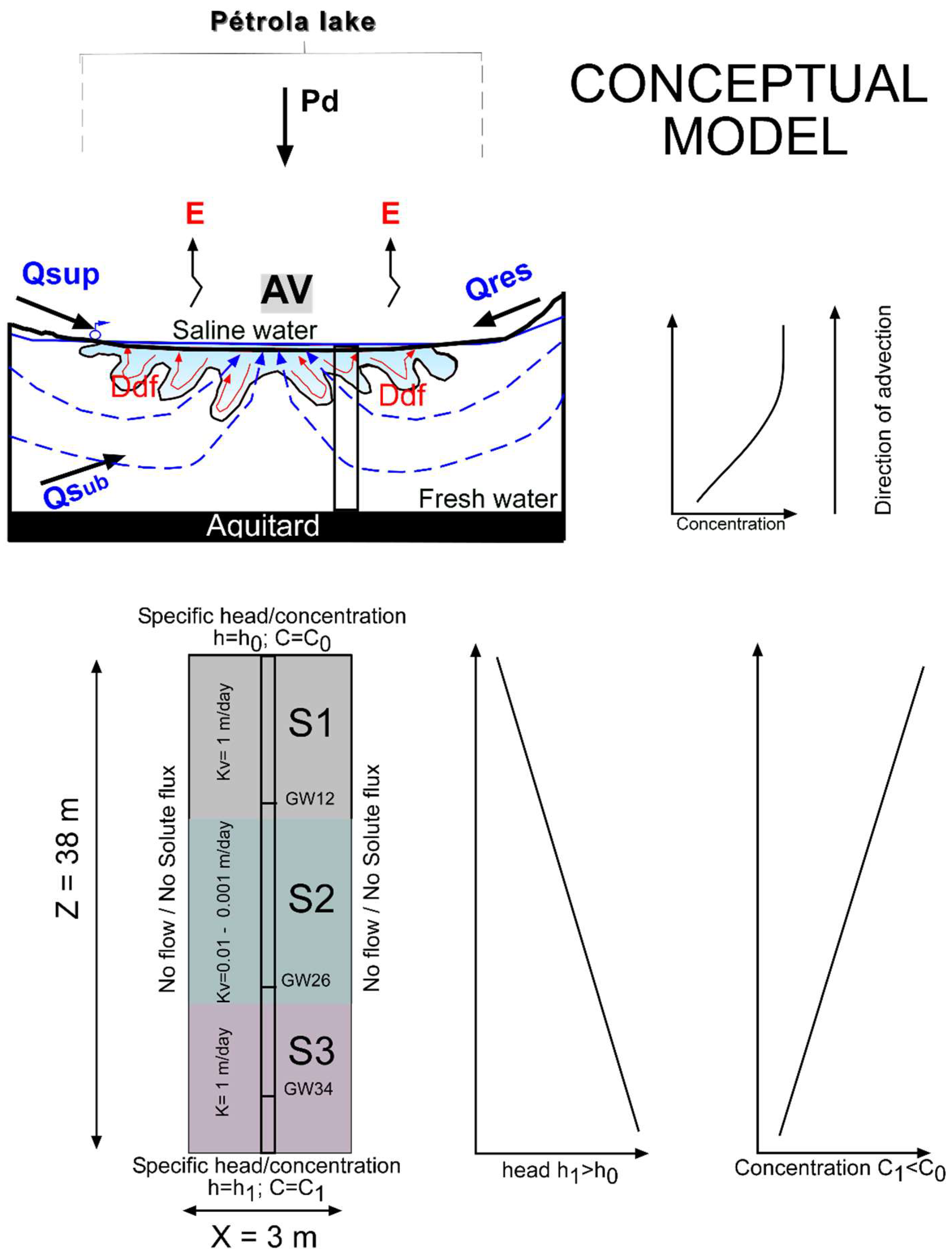
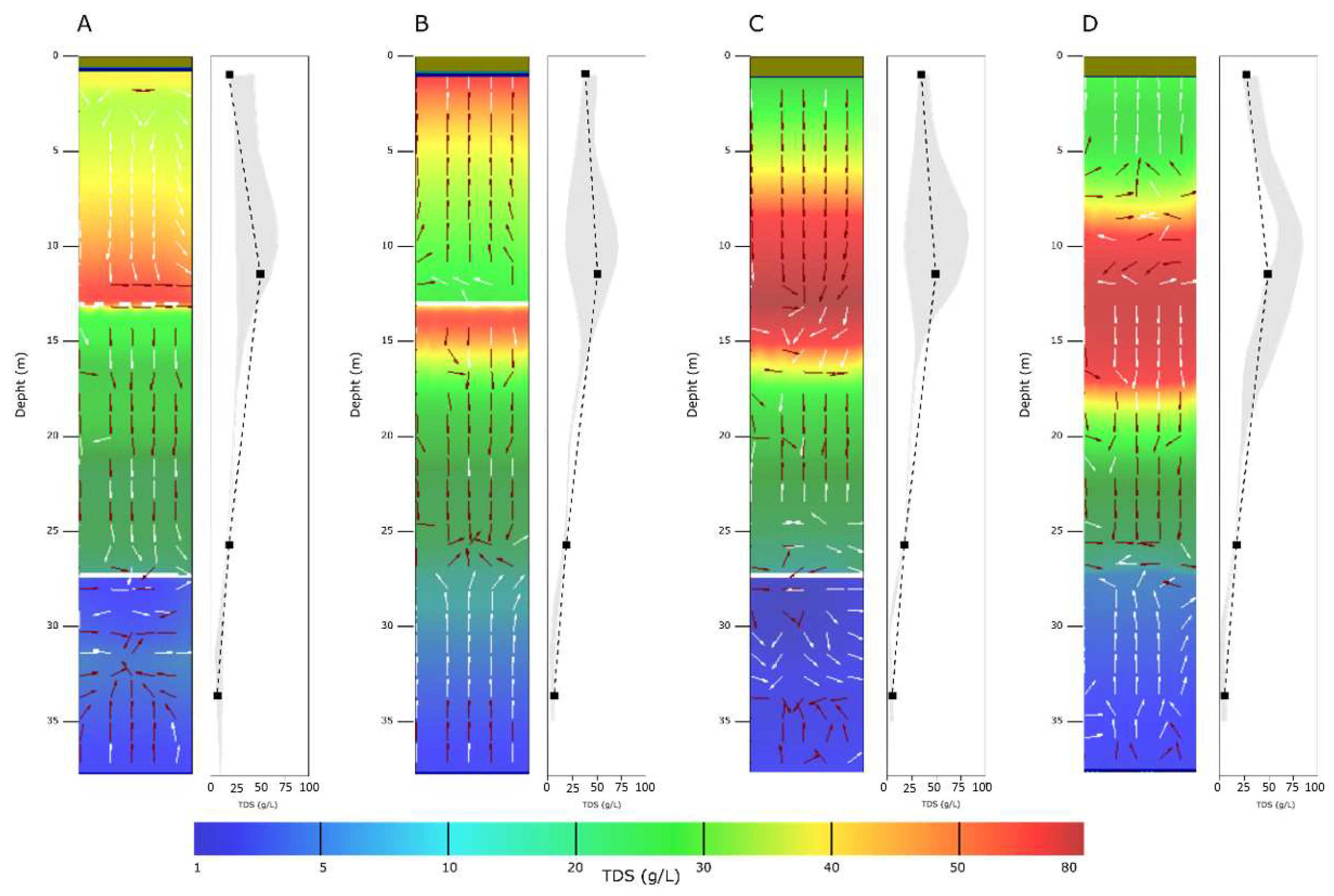
4.3. Feasibility of the Hydrochemical Conceptual Model

Based on the above observations, a conceptual model of the hypersaline Pétrola Lake over a freshwater aquifer is represented (Figure 5). The hydraulic potential of the aquifer (h₁, equivalent freshwater head, corrected through the groundwater level and the TDS) is higher than the lake’s surface water level (h₀). Therefore, the direction of the RGF would convert the lake into a discharge zone. On the other hand, the lake’s mean salinity is up to 20 times higher than the aquifer’s salinity, which can generate gravitational instability causing a DDF from the lake towards the underlying aquifer [48]. Previous studies have used the mixed convection ratio (Equation (10)) as a predictor of the probability of a downward flow occurring driven by density differences (see [14,49]).

M = [(ρ_s − ρ_o)/ρ_o]/(∆h/∆z),

(10)

where ρ_s is the density of hypersaline water from the lake; ρ_o is the freshwater density from the aquifer; and (∆h/∆z) is the hydraulic head gradient. The threshold of m = 1 marks the boundary between advection (m < 1) and density-driven flow (m > 1)-dominated simulations. This simplification is valid for homogeneous and isotropic media and with changes in semi-steady-state conditions. However, this does not occur in the case at hand, where both the heterogeneity of the medium and the variation in time of the boundary conditions make it difficult to understand the operation of both processes over time.

In order to establish the mechanisms that govern the variability of both the RGF and DDF, a simple geometrical configuration was made. Specifically, a one-dimensional column that represents the vertical flow (coinciding with the position of the GW-12, GW-26, and GW-34 piezometers). Since groundwater flow paths directly below the surface water body are sub-vertical to vertical, horizontal flow is not considered in this analysis. For this, a numerical model was implemented in a column 38 m deep and 3 m wide that shows the relationship between the lake and the aquifer as the final groundwater discharge point. The distribution of the hydraulic parameters was obtained from the lithological characterisation of the piezometers and is similar to the data used in [21] (Figure 5). The variable-density groundwater flow and solute transport were simulated numerically using SEAWAT [50,51], which solves the general equation of flow and transport in porous media with density differences. The model was discretised with a uniform mesh in square cells of ∆x = 0.25m; and ∆z = 0.25m. The boundary conditions were implemented as type 1 (constant head) for flow and transport and taken from the information from the piezometers (GW-12 and GW-34, Figure 2). The top of the column represents the boundary conditions of the lake (h₀: constant head and C₀: TDS concentration), whereas the bottom of the column represents the regional flow of the aquifer (h₁, C₁). The model assumes invariant conditions from an isothermal and fluid viscosity point of view. A complete list of the parameters used can be seen in

Table 2. Model parameters for numerical simulations: horizontal hydraulic conductivity (Kh), anisotropy ratio (Kv/Kh = 1/10), specific storage (Ss), porosity (n), effective molecular diffusivity (Dm), longitudinal dispersivity (αL), and transverse dispersivity (αT), effective molecular diffusion (Dm), for the upper sandy sediments aquifer (S1), mid argillaceous sediments aquitard (S2), lower sandy sediments aquifer (S3), based on [21].

Parameter	Value	Dimension
Kv (S1)	1	[m/day]
Kv (S2)	0.01–0.001	[m/day]
Kv (S3)	1	[m/day]
Ss	1 × 10−5	[-]
n	0.3	[-]
αL	0.1	[m]
αT	0.01	[m]
Dm	1 × 10−5	[m2/s]

. The time steps are restricted in SEAWAT by the Peclet criterion that was set to 0.1. The stress periods were taken daily to represent the periods studied in Figure 2 (January 2010–November 2011). The initial conditions were established based on the head potential and TDS values from January 2010.

The vertical distribution of salinity together with the flow directions, confirm the hydrogeochemical conceptual model of the saltwater–aquifer relationships (Figure 6). The simulation results have been grouped into four characteristic periods. The first period (Figure 6A) represents the period from January 2010 to June 2010. The simulation shows how the TDS concentrations were higher in GW-12 than in the surface water. The flow lines corroborate the possibility that the heaviest δ¹⁸O_H2O values in the piezometers were found. During the second period (from July 2010 to April 2011, Figure 6B), eminently dry, the simulation confirms the hydrogeochemical data showing higher salinity contents in the surface water than in the groundwater (GW-12). This fact, together with the decreasing trend in the head potentials in both the lake and GW-12, provokes a downward flow towards GW-26, therefore increasing the groundwater level in GW-26 (Figure 2). Regarding the isotopic data at the end of this period, they indicated the minimum differences between the surface water and GW-12 in δ¹⁸O_H2O. The third period (from May 2011 to July 2011, Figure 6C) represents a very humid period, where the lake head potential increases considerably (even above the head potential in GW-34) but with lower salinities in the surface water than in GW-12. From this period, there are no hydrochemical and isotopic data, but convection cells are observed at different depths beyond the lake, caused by the heterogeneity of the medium and the adaptation to the changing boundary conditions. Finally, the fourth period (from August 2011 to October 2011, Figure 6D) shows the transition from the intensely humid period to the initial conditions shown in Figure 6A.

In general, the simulations show that salinity variations vary more on the surface than with the depth, showing a decrease with the depth throughout the simulation period. The arrangement of the depth permeability differences plays a determining role in the movement of solutes due to the density differences. In the zones with the highest permeability (0–12 mbgs) the salinity variations are very irregular. In areas of lower permeability (12–28 mbgs), an attenuation of fluxes of variable densities occurs and the salinity showed much less variability. The area of the aquifer with the freshwater maintains a practically constant head potential and salinity, which implies that the RGF could be much larger than the DDF. However, the variations in the head potential and salinity of the surface water in the lake together with the heterogeneity of the media means that the system is in equilibrium between the DDF and RGF.

5. Conclusions

The study of the interactions between saline lakes and underlying aquifers is essential for improving the knowledge of the nature of reactive processes in these systems (e.g., mineral precipitation, pollutants attenuation). In our study, a strong connection between surface water and groundwater is evident from chemical, isotopic, and modelling data. The isotopic data showed that evaporation is one of the governing processes in the Pétrola lake–aquifer system, taking place at humidity values of about 68%. Groundwater recharge was mainly related to Atlantic precipitation, but the δ¹⁸O_H2O and δ²H_H2O values also reflected the mixing processes occurring between the surface lake water (evaporated) and the regional groundwater flowing in from below. The important variations observed in Cl⁻, δ¹⁸O_H2O, and δ²H_H2O on the surface were not observed in the groundwater as both the lake and groundwater are under steady-state conditions. The buoyancy of the RGF upwards limits the impact of the DDF in solute transport. The numerical flow and transport model showed that the lake’s influence is stronger when the groundwater potential decreases, coinciding with the lowest density values on the surface. Our results showed that there is a time lag between lake and aquifer events, the first strongly influencing the geochemical characteristics of springs and streams around the lake. It supports the fact that the FSI can constitute a natural barrier to the natural attenuation of pollutants when the biogeochemical conditions are suitable.

Additional field information and well monitoring are needed to estimate the rate of mass transport during the density-driven groundwater flow. The study of the Pétrola lake–aquifer system offers an opportunity to identify the complex chemical and physical parameters in saline aquifer systems, including the various possible factors that can degrade groundwater quality or attenuate pollutants. Despite being a particular case study, it is sufficient to highlight the geologically controlled exchange processes expected to occur in other hypersaline lakes around the world.

References

1. Shiklomanov, I.A.; Rodda, J.C. World Water Resources at the Beginning of the Twenty-First Century; Cambridge University Press: Cambridge, UK, 2004. [Google Scholar]
2. Yechieli, Y.; Wood, W.W. Hydrogeologic processes in saline systems: Playas, sabkhas, and saline lakes. Earth-Sci. Rev. 2002, 58, 343–365. [Google Scholar] [CrossRef]
3. Macumber, P.G. Interaction between Groundwater and Surface Systems in Northern Victoria; Department of Conservation and Environment: Melbourne, VIC, Australia, 1991.
4. Herczeg, A.L.; Barnes, C.J.; Macumber, P.G.; Olley, J.M. A stable isotope investigation of groundwater-surface water interactions at Lake Tyrrell, Victoria, Australia. Chem. Geol. 1992, 96, 19–32. [Google Scholar] [CrossRef]
5. Wooding, R.A.; Tyler, S.W.; White, I.; Anderson, P.A. Convection in groundwater below an evaporating Salt Lake: 2. Evolution of fingers or plumes. Water Resour. Res. 1997, 33, 1219–1228. [Google Scholar] [CrossRef]
6. Dutkiewicz, A.; Herczeg, A.L.; Dighton, J.C. Past changes to isotopic and solute balances in a continental playa: Clues from stable isotopes of lacustrine carbonates. Chem. Geol. 2000, 165, 309–329. [Google Scholar] [CrossRef]
7. Cartwright, I.; Hall, S.; Tweed, S.; Leblanc, M. Geochemical and isotopic constraints on the interaction between saline lakes and groundwater in southeast Australia. Hydrogeol. J. 2009, 17, 1991–2004. [Google Scholar] [CrossRef]
8. Levy, Y.; Burg, A.; Yechieli, Y.; Gvirtzman, H. Displacement of springs and changes in groundwater flow regime due to the extreme drop in adjacent lake levels: The Dead Sea rift. J. Hydrol. 2020, 587, 124928. [Google Scholar] [CrossRef]
9. Torgersen, T.; De Deckker, P.; Chivas, A.; Bowler, J. Salt Lakes: A discussion of processes influencing palaeoenvironmental interpretation and recommendations for future study. Palaeogeogr. Palaeoclim. Palaeoecol. 1986, 54, 7–19. [Google Scholar] [CrossRef]
10. Duffy, C.J.; Al-Hassan, S. Groundwater circulation in a closed desert basin: Topographic scaling and climatic forcing. Water Resour. Res. 1988, 24, 1675–1688. [Google Scholar] [CrossRef]
11. Nicolás, V.; Jirsa, F.; Gómez-Alday, J.J. Saline lakes as barriers against pollution: A multidisciplinary overview. Limnetica 2022, 41. [Google Scholar] [CrossRef]
12. Gómez-Alday, J.; Carrey, R.; Valiente, N.; Otero, N.; Soler, A.; Ayora, C.; Sanz, D.; Muñoz-Martín, A.; Castaño, S.; Recio, C.; et al. Denitrification in a hypersaline lake–aquifer system (Pétrola Basin, Central Spain): The role of recent organic matter and Cretaceous organic rich sediments. Sci. Total Environ. 2014, 497–498, 594–606. [Google Scholar] [CrossRef]
13. Valiente, N.; Carrey, R.; Otero, N.; Soler, A.; Sanz, D.; Muñoz-Martín, A.; Jirsa, F.; Wanek, W.; Gómez-Alday, J. A multi-isotopic approach to investigate the influence of land use on nitrate removal in a highly saline lake-aquifer system. Sci. Total Environ. 2018, 631–632, 649–659. [Google Scholar] [CrossRef] [PubMed]
14. Massmann, G.; Simmons, C.; Love, A.; Ward, J.; James-Smith, J. On variable density surface water–groundwater interaction: A theoretical analysis of mixed convection in a stably-stratified fresh surface water—Saline groundwater discharge zone. J. Hydrol. 2006, 329, 390–402. [Google Scholar] [CrossRef]
15. Bentley, L.R.; Hayashi, M.; Zimmerman, E.P.; Holmden, C.; Kelley, L.I. Geologically controlled bi-directional exchange of groundwater with a hypersaline lake in the Canadian prairies. Hydrogeol. J. 2016, 24, 877–892. [Google Scholar] [CrossRef]
16. Pham, S.V.; Leavitt, P.R.; McGowan, S.; Wissel, B.; Wassenaar, L. Spatial and temporal variability of prairie lake hydrology as revealed using stable isotopes of hydrogen and oxygen. Limnol. Oceanogr. 2009, 54, 101–118. [Google Scholar] [CrossRef]
17. Cendón, D.I.; Larsen, J.; Jones, B.; Nanson, G.C.; Rickleman, D.; Hankin, S.I.; Pueyo, J.J.; Maroulis, J. Freshwater recharge into a shallow saline groundwater system, Cooper Creek floodplain, Queensland, Australia. J. Hydrol. 2010, 392, 150–163. [Google Scholar] [CrossRef]
18. Valiente, N.; Carrey, R.; Otero, N.; Gutiérrez-Villanueva, M.A.; Soler, A.; Sanz, D.; Castaño, S.; Gómez-Alday, J.J. Tracing sulfate recycling in the hypersaline Pétrola Lake (SE Spain): A combined isotopic and microbiological approach. Chem. Geol. 2017, 473, 74–89. [Google Scholar] [CrossRef]
19. Jódar, J.; Rubio, F.; Custodio, E.; Martos-Rosillo, S.; Pey, J.; Herrera, C.; Turu, V.; Pérez-Bielsa, C.; Ibarra, P.; Lambán, L. Hydrogeochemical, isotopic and geophysical characterization of saline lake systems in semiarid regions: The Salada de Chiprana Lake, Northeastern Spain. Sci. Total Environ. 2020, 728, 138848. [Google Scholar] [CrossRef]
20. Martino, P.; Montes del Olmo, C.; Alonso, M. Sobre La Conservación y Gestión de Las Lagunas Salados En España. In Proceedings of the I: Ponencias y Comunicaciones. II: Conclusiones y Participantes/Jornadas Sobre la Conservación de la Naturaleza en España, Oviedo, Spain, 27 November 1986; pp. 235–238. [Google Scholar]
21. Sanz, D.; Valiente, N.; Dountcheva, I.; Muñoz-Martín, A.; Cassiraga, E.; Gómez-Alday, J.J. Geometry of the modelled freshwater/salt-water interface under variable-density-driven flow (Pétrola Lake, SE Spain). Hydrogeol. J. 2022, 30, 975–988. [Google Scholar] [CrossRef]
22. Ordóñez, S.; García del Cura, M.A.; Marfil, S. Sedimentación actual: La laguna de Pétrola (Albacete). Estud. Geológicos 1973, 29, 367–377. [Google Scholar]
23. Donate, J.A.L.; Ibáñez, J.G.M.; Cano, J.A.L.; Núñez, J.C.M. Estudio Descriptivo Del Sector Endorreico-Salino de Pétrola, Corral Rubio y La Higuera (Albacete). In Proceedings of the Jornadas Sobre el Medio Natural Albacetense, Instituto de Estudios Albacetenses “Don Juan Manuel”, Albacete, Spain, 28 November 2001; pp. 357–370. [Google Scholar]
24. APHA WEF AWWA. Standard Methods for the Examination of Water and Wastewater; APHA WEF AWWA: Washington, DC, USA, 2005. [Google Scholar]
25. Santoyo, E.; García, R.; Abella, R.; Aparicio, A.; Verma, S. Capillary electrophoresis for measuring major and trace anions in thermal water and condensed-steam samples from hydrothermal springs and fumaroles. J. Chromatogr. A 2001, 920, 325–332. [Google Scholar] [CrossRef]
26. Calmbach, L. AquaChem Computer Code, Version 3.7. 42; Waterloo Hydrogeologic, Inc.: Waterloo, ON, Canada, 1997.
27. Araguas, L.A.; Danesi, P.; Froehlich, K.; Rozanski, K. Global monitoring of the isotopic composition of precipitation. J. Radioanal. Nucl. Chem. Artic. 1996, 205, 189–200. [Google Scholar] [CrossRef]
28. Jouzel, J.; Froehlich, K.; Schotterer, U. Deuterium and oxygen-18 in present-day precipitation: Data and modelling. Hydrol. Sci. J. 1997, 42, 747–763. [Google Scholar] [CrossRef]
29. Gonfiantini, R. Environmental Isotopes in Lake Studies. Handb. Environ. Isot. Geochem. Terr. Environ. 1986, 2, 113–168. [Google Scholar]
30. Gammons, C.H.; Poulson, S.R.; Pellicori, D.A.; Reed, P.J.; Roesler, A.J.; Petrescu, E.M. The hydrogen and oxygen isotopic composition of precipitation, evaporated mine water, and river water in Montana, USA. J. Hydrol. 2006, 328, 319–330. [Google Scholar] [CrossRef]
31. Majoube, M. Fractionnement En Oxygène 18 et En Deutérium Entre l’eau et Sa Vapeur. J. Chim. Phys. 1971, 68, 1423–1436. [Google Scholar] [CrossRef]
32. Horita, J.; Wesolowski, D.J. Liquid-vapor fractionation of oxygen and hydrogen isotopes of water from the freezing to the critical temperature. Geochim. Cosmochim. Acta 1994, 58, 3425–3437. [Google Scholar] [CrossRef]
33. Jacob, H.; Sonntag, C. An 8-year record of the seasonal variation of 2H and 18O in atmospheric water vapour and precipitation at Heidelberg, Germany. Tellus B Chem. Phys. Meteorol. 1991, 43, 291–300. [Google Scholar] [CrossRef] [Green Version]
34. Bethke, C. The Geochemists Workbench, v. 6.0; University of Illinois: Champaign, IL, USA, 2006.
35. Vandenschrick, G.; van Wesemael, B.; Frot, E.; Pulido-Bosch, A.; Molina, L.; Stiévenard, M.; Souchez, R. Using stable isotope analysis (δD–δ18O) to characterise the regional hydrology of the Sierra de Gador, south east Spain. J. Hydrol. 2002, 265, 43–55. [Google Scholar] [CrossRef]
36. Dansgaard, W. Stable Isotopes in Precipitation. Tellus 1964, 16, 436–468. [Google Scholar] [CrossRef]
37. Uemura, R.; Matsui, Y.; Yoshimura, K.; Motoyama, H.; Yoshida, N. Evidence of deuterium excess in water vapor as an indicator of ocean surface conditions. J. Geophys. Res. Earth Surf. 2008, 113, D19114. [Google Scholar] [CrossRef] [Green Version]
38. Julian, J.C.-S.; Araguas, L.; Rozanski, K.; Benavente, J.; Cardenal, J.; Hidalgo, M.C.; García-López, S.; Martinez-Garrido, J.C.; Moral, F.; Olías, M. Sources of precipitation over South-Eastern Spain and groundwater recharge. An isotopic study. Tellus B Chem. Phys. Meteorol. 1992, 44, 226–236. [Google Scholar] [CrossRef] [Green Version]
39. Ciric, D.; Nieto, R.; Losada, L.; Drumond, A.; Gimeno, L. The Mediterranean Moisture Contribution to Climatological and Extreme Monthly Continental Precipitation. Water 2018, 10, 519. [Google Scholar] [CrossRef] [Green Version]
40. Hatvani, I.G.; Erdélyi, D.; Vreča, P.; Kern, Z. Analysis of the Spatial Distribution of Stable Oxygen and Hydrogen Isotopes in Precipitation across the Iberian Peninsula. Water 2020, 12, 481. [Google Scholar] [CrossRef] [Green Version]
41. Araguas-Araguas, L.; Diaz Teijeiro, M. Isotope Composition of Precipitation and Water Vapour in the Iberian Peninsula: First Results of the Spanish Network of Isotopes in Precipitation. Int. At. Energy Agency Tech. Rep. 2005, 1453, 173–190. [Google Scholar]
42. Habeck-Fardy, A.; Nanson, G.C. Environmental character and history of the Lake Eyre Basin, one seventh of the Australian continent. Earth-Sci. Rev. 2014, 132, 39–66. [Google Scholar] [CrossRef] [Green Version]
43. Alvarez, M.D.P.; Carol, E.; Eymard, I.; Bilmes, A.; Ariztegui, D. Hydrochemistry, isotope studies and salt formation in saline lakes of arid regions: Extra-Andean Patagonia, Argentina. Sci. Total Environ. 2022, 816, 151529. [Google Scholar] [CrossRef]
44. Krause, S.; Lewandowski, J.; Grimm, N.B.; Hannah, D.M.; Pinay, G.; McDonald, K.; Martí, E.; Argerich, A.; Pfister, L.; Klaus, J.; et al. Ecohydrological interfaces as hot spots of ecosystem processes. Water Resour. Res. 2017, 53, 6359–6376. [Google Scholar] [CrossRef] [Green Version]
45. Lau, M.P.; Niederdorfer, R.; Sepulveda-Jauregui, A.; Hupfer, M. Synthesizing redox biogeochemistry at aquatic interfaces. Limnologica 2018, 68, 59–70. [Google Scholar] [CrossRef] [Green Version]
46. Badve, R.; Kumaran, K.; Rajshekhar, C. Eutrophication of Lonar Lake, Maharashtra. Curr. Sci. 1993, 65, 347–351. [Google Scholar]
47. Zimmermann, S.; Bauer, P.; Held, R.; Kinzelbach, W.; Walther, J. Salt transport on islands in the Okavango Delta: Numerical investigations. Adv. Water Resour. 2006, 29, 11–29. [Google Scholar] [CrossRef]
48. Liu, Y.; Kuang, X.; Jiao, J.J.; Li, J. Numerical study of variable-density flow and transport in unsaturated–saturated porous media. J. Contam. Hydrol. 2015, 182, 117–130. [Google Scholar] [CrossRef] [PubMed]
49. Post, V.E.; Houben, G.J. Density-driven vertical transport of saltwater through the freshwater lens on the island of Baltrum (Germany) following the 1962 storm flood. J. Hydrol. 2017, 551, 689–702. [Google Scholar] [CrossRef]
50. Guo, W.; Langevin, C.D. User’s Guide to SEAWAT; A Computer Program for Simulation of Three-Dimensional Variable-Density Ground-Water Flow; U.S. Geological Survey: Tallahassee, FL, USA, 2002.
51. Langevin, C.D.; Thorne, D.T., Jr.; Dausman, A.M.; Sukop, M.C.; Guo, W. SEAWAT Version 4: A Computer Program for Simulation of Multi-Species Solute and Heat Transport; Techniques and Methods; U.S. Geological Survey: Tallahassee, FL, USA, 2008.
Figure 1. Hydrogeological map modified from [21]. Groundwater-level contour map over hillshade. Sample points for 2008–2010 and 2013–2015 campaigns are also given. The sketches summarise processes around the discharge flow lake type and show regions where evaporated water from the lakes mixes with the through-flowing groundwater. (A) Location of the study area. (B) Hydrochemical zonation. (C) Piezometers that monitor different depths of the aquifer under the lake, and photograph of the location of the piezometers. (S1) upper sandy sediments aquifer, (S2) mid argillaceous sediments aquitard, (S3) down sandy sediments aquifer.
Water 14 01628 g001
Figure 2. Groundwater-level evolution in the piezometers GW-12, GW-26, and GW-34 for the period February 2010–October 2011. See location in Figure 1. Bars indicate mean monthly precipitation (mm) values. Mbgs: meters below ground surface (adapted from [18]).
Water 14 01628 g002
Figure 3. Piper diagram showing the chemical composition of the water samples during the studied period.
Water 14 01628 g003
Figure 4. δ2H–δ18O diagram showing the isotope data and the Local Meteoric Water Line for the Pétrola Basin. In addition, meteoric water lines for Madrid (blue) and Murcia (green) from precipitation samples (GNIP data; [27]) are represented.
Water 14 01628 g004
Figure 5. Simplified conceptual model of the relationship between hypersaline lake and freshwater from the aquifer. The implementation of the numerical model is shown at the bottom; the equivalent freshwater potential (h1) of groundwater is greater than that of the lake (h0). However, the concentration (C0) in the lake is ostensibly higher than the concentration in the underlying aquifer. The shape of the depth profiles is assumed to be unknown and nonlinear due to the heterogeneities of the media. (S1) upper sandy sediments aquifer, (S2) mid argillaceous sediments aquitard, (S3) down sandy sediments aquifer. (DDF) density-driven flow, (Qres) wastewater, (Qsup) surface runoff, (Qsub) subsurface runoff, AV water volume change, I evaporation, (Pd) direct precipitation. Locations of piezometers are in Figure 1.
Water 14 01628 g005
Figure 6. Profile of TDS concentrations versus depth (meters below ground surface) for different periods of the simulation (see Figure 2). (A) From January 2010 to June 2010 (i.e., 15 April); (B) From July 2010 to April 2011 (i.e., 15 September); (C) From May 2011 to July 2011 (i.e., 15 June); (D) From August 2011 to October 2011 (i.e., 15 September). Black squares: Mean values of TDS-calculated data (see Table 1) are shown for the surface water, GW-12, GW-26, and GW-34 together with light-grey-shaded area which represents the concentration range covered in the respective period by the minimum values simulated along with each model layer.
Water 14 01628 g006