Framework for Dynamic Modelling of the Dam and Reservoir System Reduced Functionality in Adverse Operating Conditions

Abstract

Dam and reservoir systems (DRSs) are crucial aspects of the infrastructure necessary for reliable water resource management. Nowadays, DRSs are being increasingly affected by numerous natural and anthropogenic impacts (aging and outdated infrastructure, climate change, natural hazards, global crises, etc.). Hence, additional pressure on DRS management is being applied as DRSs must be operated in adverse operating conditions, outside of their design envelopes. Since there is no practical way to redesign DRSs to meet all possible adverse conditions, efficient simulation tools are necessary for various “what-if” analyses. A system dynamics (SD) approach can be used, as it has shown the capacity to comprehend the intrinsic system complexity. In this paper, an 11-step framework for the dynamic modelling of reduced functionality in a DRS and the emulation of the system operation in adverse conditions is proposed. The framework covers the system model design, input scenario generation, system simulation, and performance evaluation steps. A focus is placed on the steps related to system decomposition, the identification of failure-indicative parameters, the definition and implementation of failure functions in the subsystem dynamic models, and dynamic failure modelling. Through these steps, a novel procedure is proposed for the dynamic modelling of the DRS subsystems’ failures (reduced functionality), common in the operation of DRSs under adverse conditions. For each subsystem prone to failure, failure-indicative parameters are identified. Failure functions employing generic functionality indicators, with values spanning from 0 to 1, are suggested to modify the values of the failure-indicative parameters in simulations and emulate the component failure impacts on DRS operation. Possibilities for modelling failure modes for different subsystems, varying in nature, duration, and magnitude are discussed. Potential physical damage to the system components, increases in measurement uncertainty, and the lack of the spare parts during periods of global crisis are applied as disturbances to the Pirot DRS case study to illustrate the possibilities of the suggested framework’s application for DRS failure modelling. It was concluded that the proposed framework allowed for the detection of severe impacts on system performance, emphasizing the need for DRS dynamic failure modelling in system analysis.

1. Introduction

Dam and reservoir systems (DRSs) are critical elements of hydraulic-control infrastructure [1] used for water retention and conveyance for the purposes of hydropower generation, irrigation, water supply, water quality control, recreation, and flood protection. Since these systems allow for the spatial and temporal redistribution of water resources, they provide a major contribution to the development of the local and regional economy and well-being. Nowadays, the lack of water resource availability is forcing society to consider approaches to utilizing remaining, marginal water resources, with the emphasis being shifted from the supply towards the demand side of the balance equation [2].

The safety of DRSs is of paramount importance to asset owners, stakeholders, and local populations, as dam failures and dam safety incidents can lead to catastrophic events [3]. Furthermore, possible dysfunctionalities in the DRS related to the partial/temporary failure of some of the DRS components or DRS intended functionality, (e.g., the failure to deliver the required hydropower), can significantly affect the industrial and municipal sectors [4].

The term “dam failure” is defined by FEMA [5] as the sudden rapid and uncontrolled release of impounded water or liquid-borne solids, while lesser dam failures are recognized as any malfunction or abnormality outside the design assumptions and parameters that adversely affect a dam’s primary function of impounding water. It has been shown that existing dams have been exposed in last decade or two to increasing failure risks [6,7,8,9]. The risks stem mainly from aging, outdated infrastructure not meeting modern design standards and ever-changing climate conditions, which have not been addressed properly in design and management processes. Here, the focus is on the operation of the DRS in adverse conditions, where dam failure (e.g., dam breach) is not occurring, but the system’s intended functionality is challenged by an endogenous or exogenous disturbance. To allow for the mitigation or even elimination of the potential losses in these cases (life, economic, environmental), it is important for asset owners to have a good understanding of how these systems will function under all potential operating conditions [1,3,10,11,12].

In general, DRS adverse operating conditions can be induced by a wide variety and combination of events, including natural disturbances (e.g., earthquakes), out-of-range or unidentified inflows, component failures, operational mistakes, human error, design and construction flaws, etc. While the topic of dam failure has been extensively analyzed in the literature (e.g., [13,14,15,16,17,18]), dynamic failure modelling, with an analysis of system operational failures and impacts on the economy and the environment, has received less attention [19,20,21]. Identifying, fully describing, and evaluating site-specific potential failure modes are arguably the most important steps in conducting a risk analysis [5,6,7,8,9,10,11,12,13,14,15,16,17,18,19,20,21,22]. The dam industry has commonly used some of following methods [13,23,24]: Failure Modes and Effects Analysis (FMEA), Fault Tree Analysis (FTA), Event Tree Analysis (ETA), and Partitioning Multiobjective Risk Method (PMRM). However, certain drawbacks have been attributed to these methods, such as their limited ability to deal with component interactions, multi-incident events, and nonlinear system behavior [3,13,25,26,27,28]. Komey [29] points out that these methods may be too simplified for the analysis of DRSs characterized by high levels of complexity and strong interactions between humans, infrastructure, and the environment.

An attempt to overcome the stated shortcomings, by pursuing the systems approach in the assessment of DRS operation and safety, has been proposed by several researchers [25,29,30]. To analyze the response of these highly complex systems, with a large number of interacting physical and nonphysical components, system dynamic (SD) models can be used [20,31,32,33,34]. SD models are used to simulate or mimic real-time DRS operation in “what-if” scenarios. They allow for the variation of input parameters, system structure and layout, boundaries, and initial conditions. They can also facilitate multimodel simulations, hence providing a valuable tool for the detailed analysis of the full range of the potential operating conditions. An important aspect in the system operation analysis is failure modelling, where single or multiple system components (or subsystems) are affected by a particular disturbance and have reduced functionality for a finite time period (needed to detect failure, procure material, or repair the affected components). To allow for the full utilization of the SD models in the analysis of the system response in various operating scenarios (inputs), both component functionality (capacity) reduction and the nonlinear components interaction need to be adequately captured. In the [20], a detailed description of site-specific failure modeling and component interaction is given for the analyzed case studies. However, the representation is limited to a certain level of SD model details and to a fixed, daily temporal resolution. A general and more flexible approach, governed by a framework consisting of 11 steps, is suggested here. This framework introduces the steps covering the decomposition of the system into mathematically represented subsystems, failure-indicative parameter identification, and failure function definition and implementation, to allow for the dynamic failure modelling of the DRS subsystems and components. To instigate the failures of the DRS components, the use of failure functions with a generic functionality indicator, as a function variable spanning from 0 to 1, is proposed. Depending on the available information regarding the system component characteristics, data monitoring, operating rules, and failure history, as well as the goal of the analysis, the user can define multiple, separate SD models of the same DRS, or a part of it, with differing levels of details. The framework suggested here can be applied to any level of modelling detail, in which crucial system components can be defined and mathematically represented, where the increase in model details will lead to a more accurate representation of the system behavior and improved failure modelling capabilities (and a higher computational burden).

The paper is structured in the following manner: first, in the Materials and Methods section, an overview of the proposed framework is presented. Second, the system model design block is discussed, with a particular emphasis on the novel aspects of the identification of failure-indicative parameters and the component failure implementation through failure functions. Afterwards, the generation of the input scenarios is analyzed, followed by a brief elaboration of the possible methods for conducting system performance evaluations. The Materials and Methods section closes with a presentation of the case study on the Pirot DRS. In the Results section, a sample design for the relatively simple Pirot DRS dynamic model and input disturbance scenarios is given, followed by a brief analysis of the Pirot DRS’s behavior in chosen adverse conditions. The effects of the disturbances on the DRS’s intended functionalities are highlighted to illustrate the advantage of the proposed framework and the need for the dynamic failure modelling. Finally, a discussion of the results is provided, and general conclusions are derived.

2. Materials and Methods

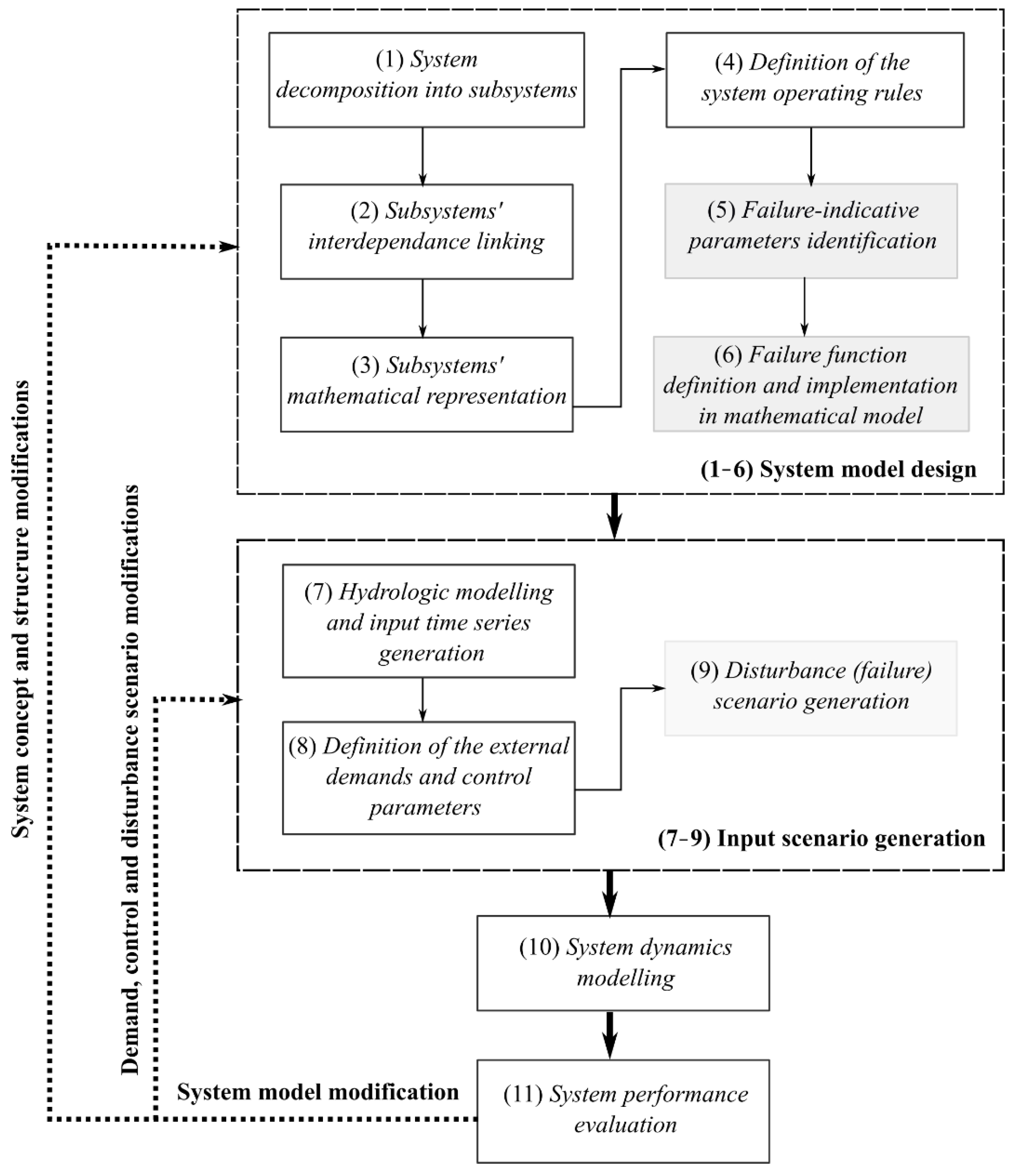
2.1. Framework Overview

A system dynamics (SD) approach has proven to be a helpful concept for long-term DRS operation simulation and analysis. To assess a system’s performance in different undesired scenarios and its capability to recover or bounce back after a disturbance event (e.g., resilience), a system component failure model must be embedded in a SD model. Even though there is research addressing this issue [20,21,31,34], there is still a necessity for a systematic, generic procedure. Therefore, in this paper, a generic, straight-forward framework for modelling DRS failure dynamics, with a great degree of flexibility, is proposed. The framework defines 11 steps (Figure 1). Steps 1–6 cover the system model design: (1) System decomposition into the subsystems where crucial components and processes must be identified; (2) Subsystems interdependence linking, where input/output for each subsystem must be assigned; (3) Subsystems’ mathematical representation, where the transformation of the inputs to the outputs must be emulated using equations (e.g., balance equation, dynamic equation) of appropriate complexity; (4) Definition of the system operating rules, describing how the monitored information is used to make operating decisions (e.g., the relations between the process and control variables); (5) Failure-indicative parameter identification, where variables indicating the reduced functionality of each subsystem prone to failure must be detected; and (6) Failure function definition and implementation in a mathematical model where the relation (failure function) between the failure-indicative parameter and a generic functionality indicator is defined, through which the functionality indicator can affect the value of the failure-indicative parameter and emulate the subsystems’ reduced functionality (partial failure). It is assumed that the used SD models have at least a minimal level of detail needed for the execution of Steps 1–6. Over-simplified and fully stochastic models cannot be used, as they will fall short in the definition of the nonlinear component interaction.

Steps 7–9 cover the input scenario generation: (7) Hydrologic modelling of the watershed and the long inflow time-series generation or inflow forecasting; (8) Definition of external demands and characteristic control trigger values (e.g., maximum and minimum reservoir levels for power production); (9) Disturbance (failure) scenario generation, where a wide range of operating scenarios is generated, including a single or a combination of system disturbances, varying in magnitude and time, and affecting the system performance, are generated. SD modelling (10) is next, where a simulation model is used to emulate system behavior under different input scenarios. Using the output results from Step 10, system performance evaluation should be conducted (Step 11). Based on the performance evaluation, SD model modifications can be performed, for example to investigate the effects of the increase in the external demands, or to analyze the behavior of the upgraded DRS with new or modified system components and operating rules. If structural modifications are needed, all the previous procedure steps should be revisited so as to adequately implement the modification in the existing model (e.g., a new subsystem means new links, a new mathematical model, new failure-indicative parameters, etc.). Even though the same set of disturbances must be used to evaluate structural modifications in the SD model, input scenario generation (Steps 7–9) should be performed again (e.g., new failure-indicative parameters need to be incorporated into the scenarios). Otherwise, experimentation with external demands and tuning the control parameters of the existing SD model, for performance optimization, or increasing the number and type of the disturbance scenarios, require repeating only the later corresponding steps in the input-scenario block (7–11).

Descriptions of the framework steps are given in the following sections and are supplemented with illustrations and mathematical examples of the step implementation in the dam and reservoir SD models. However, since there is a very large number of possible ways that DRS dynamic models can be devised and structured, depending on the modelling strategy and the type of reservoir system, this paper cannot cover all the aspects which are deemed important in the modelling process. Examples used here are mostly correlated to hydraulic operation and system maintenance, while complementing mechanical, power, and environmental aspects are given somewhat less attention.

2.2. System Model Design

When SD modelling is used to assess a system’s performance for different hydrological and failure scenarios, appropriate conceptual and mathematical representations of each subsystem function, should be defined.

First, system decomposition is conducted (Figure 2), where the key system subsystems (Step 1), and corresponding interdependencies are identified (Step 2). Subsystems are used to describe a process or a transformation of internal and/or external inputs into outputs within the system (here, a DRS). A subsystem can correspond to a particular physical component/object within the system, but it can also serve to describe a certain process of interest, e.g., evaporation. For each subsystem, appropriate mathematical representation must be defined to represent subsystem dynamics (Step 3). Mathematical representation complexity depends on the desired levels of detail, simulation goals, time-step, and duration (time scale) of the simulation. Mathematical representations of each subsystem can be described using generalized Equation (1):

$$s{d}_i^{out}=subsystemDynamics\left(s{d}_{ij}^{inp},p_k\right)$$

(1)

where $s{d}_i^{out}$ represents subsystem output obtained using the $subsystemDynamics$ model—which models the relationship between subsystem outputs and a number of inputs. The $subsystemDynamics$ for a subsystem $i$ will transform the inputs $s{d}_{ij}^{inp}$ from other subsystems ($j$ = 1,…,N; N—number of interconnected subsystems) into a certain output $s{d}_i^{out}$. The way that subsystem i transforms $s{d}_{ij}^{inp}$ into $s{d}_i^{out}$ is governed by the model structure (mathematically, it can be deemed a product of binary functions and other mathematical expressions) and model/equation parameters $p_k$ ($k$ = 1,…,M; M—number of parameters).

Different subsystem dynamic modelling strategies can be used, varying in detail level and conceptualization approach. It should be stressed that the focus here is placed on the modelling of the subsystem’s, or component’s, reduced functionality during failure—therefore, when defining the appropriate modelling strategy for a particular subsystem, the mathematical representation should allow for such analysis. The Boolean or binary states of subsystems and subsystem components (e.g., spillway gate hoist is functional/nonfunctional—hence spillway overflow is $Q_S$ or equal to 0) must be complemented with the range of operating states “in-between”, where the subsystem still performs the input transformation although with a reduced functionality (e.g., spillway gate hoist is blocked—leaving gate in the partially open position and/or with a reduced range of opening).

For the analysis of the reduced functionality of the system components, governing water resource allocation, appropriate subsystems of the DRS model should be used to simulate the hydraulic transformation of the system inputs into the outputs. In general, the most common equations for hydraulic modelling are the mass-balance equation and some approximation of a dynamic equation (momentum conservation law). For example, subsystems with storage capacity (e.g., reservoir, tanks) should be represented using the mass-balance equation (Equation (2)) to calculate water volume changes in a reservoir or tank. The water level in storage subsystems can be evaluated using a stage-storage curve (Equation (3)). Subsystems used for water transport (e.g., power tunnel, penstock, pipeline, open channel) should be represented using a form of dynamic equation (Equation (4)). When spillways with confined flow under gates are considered, an appropriate underflow/orifice equation can be used (Equation (5)). Additionally, seepage flow through the dam body or grout curtain also affects reservoir mass-balance and, for example, can be represented in a simplified exponential form (Equation (6)). Reservoir discharge is routed downstream through the river. Depending upon the level of complexity that is required, a river subsystem can be represented using a simulation model based on the Saint-Venant equations (for more complex analysis) or by using rating curve(s) to evaluate stage hydrographs at downstream control points.

$$V_i\left(t+∆t\right)=V_i\left(t\right)+∆t·\left({\displaystyle \sum }{Q}_{in}-{\displaystyle \sum }{Q}_{out}\right)$$

(2)

$$Z_i\left(t+∆t\right)=Z\left(V_i\left(t+∆t\right)\right)$$

(3)

$$Q_{ij}=sgn\left(Z_i-Z_j\right)·\sqrt{\frac{g·{\pi }^2·D^5·\left|Z_i-Z_j\right|}{8·\lambda ·L}}$$

(4)

$$Q_s=C_Q·e·B·\sqrt{2·g·\left(Z_{res}-Z_s\right)}$$

(5)

$$Q_{seepage}=K·Z_{res}^x$$

(6)

In Equations (2)–(6), the following variables are introduced:

• $V\left(t\right)$ [m³]—current water volume in storage element (e.g., reservoir, tank) at time t;
• $Z\left(t\right)$ [m]—water level in storage element (e.g., reservoir, tank) at time t;
• $∆t$ [s]—simulation time-step;
• $Q_{in}$ [m³/s]—all the inflows for specific subsystem;
• $Q_{out}$ [m³/s]—all the outflows from specific subsystem;
• $Q_{ij}$ [m³/s]—flow in a pressurized pipeline between two storage elements;
• $Q_S$ [m³/s]—spillway underflow;
• $Q_{seepage}$ [m³/s]—seepage flow;
• $g$ [m/s²]—acceleration due to gravity;
• $D$ [m]—pipeline diameter;
• $\lambda$ [/]—Darcy–Weisbach friction coefficient;
• $L$ [m]—pipeline length;
• $C_Q$ [/]—orifice coefficient;
• $B$ [m]—crest length (spillway gate width);
• $e$ [m]—spillway gate opening height;
• $Z_{res}$ [m]—reservoir water level;
• $Z_S$ [m]—spillway level;
• $K$—seepage coefficient;
• $x$—seepage exponent.

Along with storage and transport elements, the SD modelling approach allows for the modelling of the operation, and the malfunction, of the DRS monitoring system. A number of hydraulic, mechanical, and electric control variables are typically monitored in real-time operation, providing the information needed for the operation of the reservoir system. However, in adverse operating conditions, the monitoring system failure, including the sudden or creeping increase of measurement uncertainty, can severely affect control decisions, hence leading to reductions in system functionality. An example of the modelling of the failure-indicative water-level monitoring system is given in Equation (7):

$$Z_{sensor,i}=Z_i+∆Z_{noise}+∆Z_{drift}$$

(7)

Here, $Z_{sensor,i}$ represents the sensor reading of a reservoir $i$ water level, used for making operating decisions. This value can differ from the real value $Z_i$, both due to sensor noise $∆Z_{noise}$ (statistical uncertainty), and/or zero drift error $∆Z_{drift}$ (systematic uncertainty). Depending on the time-step used in the simulation, the magnitudes of the $∆Z_{noise}$ and $∆Z_{drift}$ will vary, where, for example, on the hourly and daily basis the $∆Z_{noise}$ should be negligible (as typically the output from the level sensors is damped on a minute scale—suppressing the noise effects), while on the second and minute time-steps, the induced measurement uncertainty can be more important.

An important part of the SD model is also a control subsystem which governs the system’s operational action through changes in states of the actuators. Prior identification of the process and control variables in the mathematical model is needed to enable the implementation of the appropriate control functions in the SD model. For example, when spillway underflow is controlled by spillway gates, reservoir water level $Z$ is considered as a process variable, and it should be used as an input to the modelling block which emulates actuators. Spillway gate opening height e is the actuator’s output (control variable) in the SD model. The gate operating rule governs the change of the control variable e as a function of the process variable $Z$, where the characteristic trigger values of process variable $Z$ are deemed as control parameters. The system operating rules define how the system will function in respect to the available monitored data (which can be biased, as shown above in Equation (7)). At the system model design stage of the framework (Step 4), operational logic is incorporated in the model (control subsystem), while later in the input scenario generation, control parameters are defined. Control parameters, e.g., the trigger values, can be tuned and optimized; hence it is deemed that these values should complement the input scenario data.

The SD model should be supplemented with the maintenance subsystem, which can model the maintenance activities (inspections, repairs, and preventive maintenance). For different subsystems and varying modes of failure/activities and magnitudes, repair time $t_{r,i}$ can be defined, during which the subsystem $i$ will be out of function, and after which it will be restored to its full functionality. The repair of a component after a disturbance can be initiated if the failure is located, classified, and all the necessary material is available on site; otherwise, a procurement time $t_{proc,i}$ needs to elapse. The sum of the $t_{proc,i}$ and $t_{r,i}$ define the failure duration. If the partial failure occurs, the subsystem or a component should operate to some degree despite the failure. Additionally, the deterioration of the components due to age can be modelled, allowing for long-term forecasting of the DRS’s operability and functionality. Even the inspection and maintenance scheme can be integrated into the model through this unit where, in regular time periods, certain system components will be out of function due to inspection and/or preventive maintenance activities.

2.2.1. Identification of Failure-Indicative Parameters

When a system has been decomposed and the appropriate subsystem dynamics models have been applied, the next step (5) is to detect failure-indicative parameters in each subsystem model. The failure-indicative parameters should clearly reflect the partial failure of the subsystem in the simulations. They can be physical attributes of the subsystem (e.g., friction factor) or attributes of the potential outcomes (e.g., sensor drift, leakage magnitude), in which case, an expert engineering analysis is needed to estimate the value of a potential outcome magnitude. The change in failure-indicative parameter value simulates the reduced functionality, or an effect of the disturbance on the appropriate subsystem component. This means that characteristic quantitative parameters need to be identified, suitable for representing the disturbance effects on the DRS’s operation in the SD simulations, and thus supporting the decision-making process in the DRS management. It is important to stress that disturbances that can affect the system operation vary in nature, origin (endogenous and exogenous), etc., hence leading to a plethora of effects, including physical damage to the system components, increases in monitoring system measurement uncertainties, failures in grid power, reduced accessibility to the site, reduced availability of spare parts, etc. An example overview of some of the most common DRS components, accompanied by governing equation(s) (if applicable) and identified corresponding failure-indicative parameters, is presented in

Table 1. Common subsystems in DRSs with examples of failure-indicative parameters.

Subsystem	Mathematical Representation	Failure-Indicative Parameter(s)
Embankment	Equation (6)	Seepage coefficient K
Spillway (underflow)	Equation (5)	Spillway opening width B and/or spillway gate opening height e
Power tunnel, penstock	Equation (4)	Diameter D and/or friction coefficient λ
Power tunnel, penstock (leakage)	$Q_{out,HPP}=Q_{HPP}+Q_{leak.}$	$\mathrm{Leakage}\mathrm{outflow}{Q}_{leak.}$
HPP (powerhouse)	Equation (2)	$\mathrm{Turbine}\mathrm{flow}{Q}_{HPP}$
Water-level sensor	Equation (7)	$\mathrm{Noise}∆Z_{noise}$  $\mathrm{and}/\mathrm{or}\mathrm{zero}\mathrm{drift}\mathrm{error}∆Z_{drift}$
Maintenance unit	/	$\mathrm{Procurement}\mathrm{time}{t}_{proc}$  $\mathrm{and}/\mathrm{or}\mathrm{repair}\mathrm{time}{t}_r$

.

To represent the failure mode in the embankment and body of the dam, induced by a physical disturbance, such as an earthquake, and resulting in the decrease of the reservoir-water-impounding functionality (increase in the seepage flow), seepage coefficient $K$ can be used as a failure-indicative parameter. The spillway subsystem, can similarly be affected by a physical disturbance, leading to different failure modes. For example, the malfunction of the gate hoist on one of the spillway gates can leave the spillway gate closed; hence, the spillway opening length $B$ can be used as a failure-indicative parameter in Equation (5) to represent the resulting capacity reduction. The gate hoist can also be blocked, leaving the gate partially open, in which case the corresponding failure-indicative parameter should be $e$, also in Equation (5). When considering the physical damage, or deterioration/increase of the material roughness, in the power tunnel or turbine penstocks, failure-indicative parameters can be the conduit diameter D, or the friction coefficient $\lambda$. Physical damage to the tunnel, penstock, or penstock and main inlet valves can result in the evolution of material ruptures, leading to an increase in leakage ($Q_{leak.}$). Even turbine flow $Q_{HPP}$ can be used as the failure-indicative parameter, to model the reduced turbine capacity. Monitoring system noise and zero-drift errors, as $∆Z_{noise}$ and $∆Z_{drift}$ in Equation (7) are also applicable as failure-indicative parameters. When external, nonphysical disturbances occur, such as the recent global crisis induced by the COVID-19 pandemic or economic and conventional wars, the markets and transport infrastructure capacities are reduced; hence, the operation (and maintenance) of the DRS can be affected. Failure-indicative parameters used for modelling these effects can be the procurement and repair times, $t_{proc}$ and $t_r$, for the subsystem components. It is worthwhile to emphasize that failure-indicative parameters should be identified using the professional experience from the literature, coupled with undertaking expert elicitation by DRS managers and operators.

2.2.2. Failure Function Definition and Implementation in the Mathematical Model

The previous step enables the detection of the failure-indicative subsystem parameters. The next step (6) requires an approach to implementing partial failure modes into the subsystem dynamics equation. When multiple failure scenarios must be analyzed, with disturbances varying in nature and effects, a generic procedure for failure modelling is required. Here, the use of failure function $f\left(\alpha \right)$ is proposed where, through $f\left(\alpha \right)$, the values of failure-indicative parameters are modified. Furthermore, this research proposes a generic functionality indicator $\alpha$ [/], as a failure function variable. This indicator has values in the range 0–1 (Equation (8)):

$$\alpha =\left\{\begin{array}{cc}1,& \mathrm{subsystem}\mathrm{in}\mathrm{usual}\mathrm{operation}-\mathrm{full}\mathrm{functionality}\\ 0<\alpha <1,& \mathrm{subsystem}\mathrm{is}\mathrm{in}\mathrm{failure}\mathrm{mode}-\mathrm{partial}\mathrm{functionality}\\ 0& \mathrm{subsystem}\mathrm{is}\mathrm{in}\mathrm{failure}\mathrm{mode}-\mathrm{non}\mathrm{functional}\end{array}\right\}$$

(8)

The suggested approach allows versatility in the modelling of various partial failures for each subsystem. In a general sense, the implementation of the failure function with the functionality indicator $\alpha$ reflects on the modification of the model used to represent the subsystem dynamics:

$$s{d}_i^{out}=subsystemDynamics\left(s{d}_{ij}^{inp},f\left({\alpha }_k\right)·p_k\right)$$

(9)

where $f\left({\alpha }_k\right)$ represents a failure function with functionality indicator as a variable (index $k$ denotes functionality indicator for $k$-th failure-indicative parameter). If possible, it is preferable to define $f\left({\alpha }_k\right)$ as a simple function, which will allow for an understandable physical interpretation and implementation. In the simulations, ${\alpha }_k$ can change in time to reflect the actual state of the subsystem component, e.g., after disturbances and during the failure period (reduced performance during the disturbance and procurement time $t_{proc}$) or activities, such as maintenance and repair (repair time $t_r$). Figure 3 illustrates a hypothetical time-series of the functionality indicators $\alpha$, with different element behavior after disturbance and with or without repair time $t_r$ (e.g., water-level sensor $t_r=0$).

Again, examples can be used to illustrate the integration of the failure function $f\left({\alpha }_k\right)$ in the subsystem dynamics models. Material deterioration due to age/exploitation in the power tunnel and penstock will result in the increase in roughness. The corresponding failure function can be $1/{\alpha }_{\lambda }$; hence, this failure can be modelled as a ratio of the design roughness coefficient $\lambda$ and functionality indicator ${\alpha }_{\lambda }$ (Equation (10)). A spillway gate outage can be modeled by multiplying the opening width $B$ with ${\alpha }_B$, or $e$ ($e_{max})$ with ${\alpha }_e$ (Equation (11)) (failure function $f\left({\alpha }_k\right)={\alpha }_k$). The failure of the impounding function of the reservoir, through the increased embankment seepage flow, can be expressed with a ratio of seepage coefficient $K$ and ${\alpha }_K$ (Equation (12)). To model the varying failure modes for the water-level monitoring system, the failure-indicative parameter $∆Z_{noise}$ should be combined with rational $f\left({\alpha }_{noise}\right)=1/{\alpha }_{noise}$, while the parameter $∆Z_{drift}$ should be multiplied by failure function $f\left({\alpha }_{drift}\right)=$1−${\alpha }_{drift}$ (Equation (13)). Particularly interesting for long-term simulations of reservoir operation in adverse conditions are the nonphysical disturbances affecting the maintenance program. The resulting effects can be represented with the rational functions $f\left({\alpha }_{proc}\right)=1/{\alpha }_{proc}$ and $f\left({\alpha }_r\right)=1/{\alpha }_r$ used to increase procurement and repair times, respectively.

$$Q_{ij}=sgn\left(Z_i-Z_j\right)·\sqrt{\frac{g·{\pi }^2·{\left({\alpha }_D·D\right)}^5·\left|Z_i-Z_j\right|}{8·\left(\lambda /{\alpha }_{\lambda }\right)·L}}$$

(10)

$$Q_s=C_Q·{\alpha }_e·e·{\alpha }_B·B·\sqrt{2·g·\left(Z_{res}-Z_s\right)}$$

(11)

$$Q_{seepage}=\frac{K}{{\alpha }_K}·Z_{res}^x$$

(12)

$$Z_{sensor,i}=Z_i+\frac{∆Z_{noise}}{{\alpha }_{noise}}+\left(1-{\alpha }_{drift}\right)∆Z_{drift}$$

(13)

Again, the list of examples can be exhaustive, depending on the SD modelling approach and concerning the varying aspects of the system operation (power, mechanical, environmental, sediment control, etc.). It should be highlighted that, for each analyzed disturbance or potential combination, the modeler should define which subsystems (and respective functionality indicators) will be affected, and how they will be affected (the failure function) on the basis of the previously conducted expert analysis.

2.3. Input Scenario Generation

To simulate both short-term and long-term DRS behavior in a wide range of operating scenarios, adequate input scenarios need to be defined. Three key steps are identified and shown in Figure 1. Step 7, hydrologic modelling and inflow time-series generation should reflect the current state of the watershed hydrology, as well as expected (or “feared”) future scenarios, with increased intensities and frequency in wet (floods) and dry (droughts) periods. Common steps in this process include the analysis of the historically observed data, use of weather generators (if needed to supplement the observed data), hydrological model calibration and verification to define the specific rainfall-runoff correlation, and, finally, generation of the long-term inflow series [34].

In Step 8, external demands and control parameters need to be defined. External demands are related to the intended functionalities of the DRS and carry the information regarding the target goals for the DRS on various time-scales (e.g., power production; drinking water extraction; irrigation, etc.) issued by external control agencies. Control parameters, as a part of the system operating rules, are subject to optimization, where the modeler can tune these parameters to maximize the functionality of the DRS. Hence, the values of these parameters are deemed part of the information defining the input scenario.

Finally, Step 9, within the input-scenario-generation block, is dedicated to the disturbance (failure) scenario generation. Multiple aspects should be considered here: the nature of disturbance, its magnitude, timing, duration, affected subsystems and subsystem components, disturbance probability, and disturbance superposition. Inherently, the generation of the disturbance scenarios is a multidimensional problem, where an almost infinite search space is available when varying the above-mentioned parameters. In [3] a combinatorial procedure is suggested, supplemented by a Monte Carlo parameterization, to cover a wide range of possible operating conditions. Even though this approach enables the assessment of the DRS’s performance under numerous failure scenarios, it requires exhaustive work in creating failure-scenario combinations. Additionally, it only provides information on how the failure will affect the system’s functionality when it happens, neglecting the probability of the disturbance’s occurrence which would lead to this failure. When there is a necessity for better insight into the DRS’s behavior, a more realistic failure generator should be used as a supplement. In this case, a causal approach, where each failure is caused by some disturbance, and each disturbance is attributed with an occurrence probability, can be utilized. This failure generation approach can result in a functionality indicator time-series which can be easily implemented in the system dynamics model. This approach can provide additional information (what caused the failure and how did the failure develop) and lead to better control of the system. As this is deemed a very important subject which deserves a thorough analysis, a separate investigation addressing the above-mentioned issues will be the subject of forthcoming research.

2.4. System Performance Evaluation

Finally, Step 11 in the suggested framework is the assessment of the simulation results and evaluation of the system performance. Depending on the analysis goals, different methodologies can be used to evaluate and quantify the performance of the reservoir system. Some common quantities are typically assessed as monthly/annual energy production, lost water volume, water delivered for irrigation, water supply, etc. Furthermore, hazard, vulnerability, and risk quantities can be used for this purpose. Lately, the concept of resilience, first static and later dynamic, has emerged as the popular approach for determining the capacity of a system to operate in adverse conditions and recover from a disturbance [31,35,36]. For the assessment of a multipurpose DRS, multiparameter dynamic resilience is deemed to be more suitable [34].

System performance improvement can be achieved through investments in the system (including an increase of the system’s capacities, different water policies, monitoring system coverage and accuracy, spare part availability, etc.) or through control-parameter optimization (operating rules and optimization of the control parameters). To investigate the effects of the above-mentioned actions, appropriate modifications in the SD model should be made, after which the same (or expanded) set of input scenarios should be simulated. It should be highlighted that, when structural modifications, or changes in the nature of operating rules are planned, the whole suggested procedure framework should be revisited, (Steps 1–9; Figure 1) while the optimization of the water policy control parameters exert only the adaptations in the input-scenario-generation block (7–9).

2.5. Case Study: Pirot DRS

The proposed framework for generic, explicit failure implementation into the SD model is tested on the Pirot DRS. The Pirot DRS is located in the southeastern region of Serbia, near the city of Pirot (Figure 4). It is a multipurpose reservoir system, currently primarily used for hydropower production, flood protection at the Nišava and Visočica Rivers, and secondarily for biological and sediment control at the watershed scale. The Pirot DRS includes the following objects: the Zavoj Reservoir and dam with gated spillway and bottom outflow, power tunnel, surge tank, penstock, hydropower plant (HPP), tailrace (open channel for hydropower outflow), and compensation reservoir. The compensation reservoir is located on the right bank of the Nišava River and is designed for outflow release attenuation and to mitigate a water-level oscillation in the Nišava River. System and dam objects are presented in more details in [21,34].

An example SD model of the Pirot DRS is presented here to illustrate the procedure for devising an SD model capable of the analysis of DRS operation in adverse conditions. Depending on the time-scale and time-step in the simulations, the SD model can be simplified or more detailed. Here, a simple model is devised for the analysis of the system functionality in adverse operating conditions in respect to the hydropower production and flood management. The performance of the Pirot reservoir system is analyzed for a two-year period with an hourly simulation time-step. Thus, some of the subsystems’ performance and hydraulic transformation cannot be represented (e.g., surge-tank-level oscillations), as their performance can be modelled only when a higher time resolution is used (smaller simulation time-step).

Adverse conditions are hypothetical (but plausible) combination of various disturbances, such as an earthquake, forest fire, creeping sensor drift error, and even a global crisis event. These disturbances are randomly chosen and distributed over a two-year period, affecting a number of system components, thus reducing their intended functionality. For comparison purposes, a regular scenario is run without disturbances. The regular and adverse set of scenarios are first executed on the basic model. To improve the DRS’s performance and mitigate the disturbance impacts, a modification of the operating rules, through the control subsystem, is analyzed. Furthermore, to investigate the effects of the hypothetical Pirot DRS upgrade in terms of the construction and operation of the water intake and pipeline for the drinking water extraction, the SD model is upgraded, and a new subsystem is introduced. A complete list of examined scenarios is shown in

Table 2. Combination of examined scenarios and model variants.

Model Variants	(BM) Basic Model	(MMOR) Model—Modified Operating Rules	(MMORS) Model—Modified Operating Rules and Structure
Scenarios
(RS) Regular Scenario—no disturbances	BM-RS	MMOR-RS	MMORS-RS
(AS1) Adverse scenario 1—physical disturbances	BM-AS1	MMOR-AS1	MMORS-AS1
(AS2) Adverse scenario 2—physical disturbances + global crisis	BM-AS2	MMOR-AS2	MMORS-AS2

.

For the sake of brevity, the system performance evaluation of the Pirot DRS case study is restricted to the comparison of the common quantities, such as monthly energy production and lost water volume (where lost water represents loss of the impounded water from the Zavoj Reservoir due to seepage, leakage, and evaporation), water volume deficits (start–end time), and the ability to deliver the requested power, biological outflow, and even drinking water outflow (MMORS).

3. Results

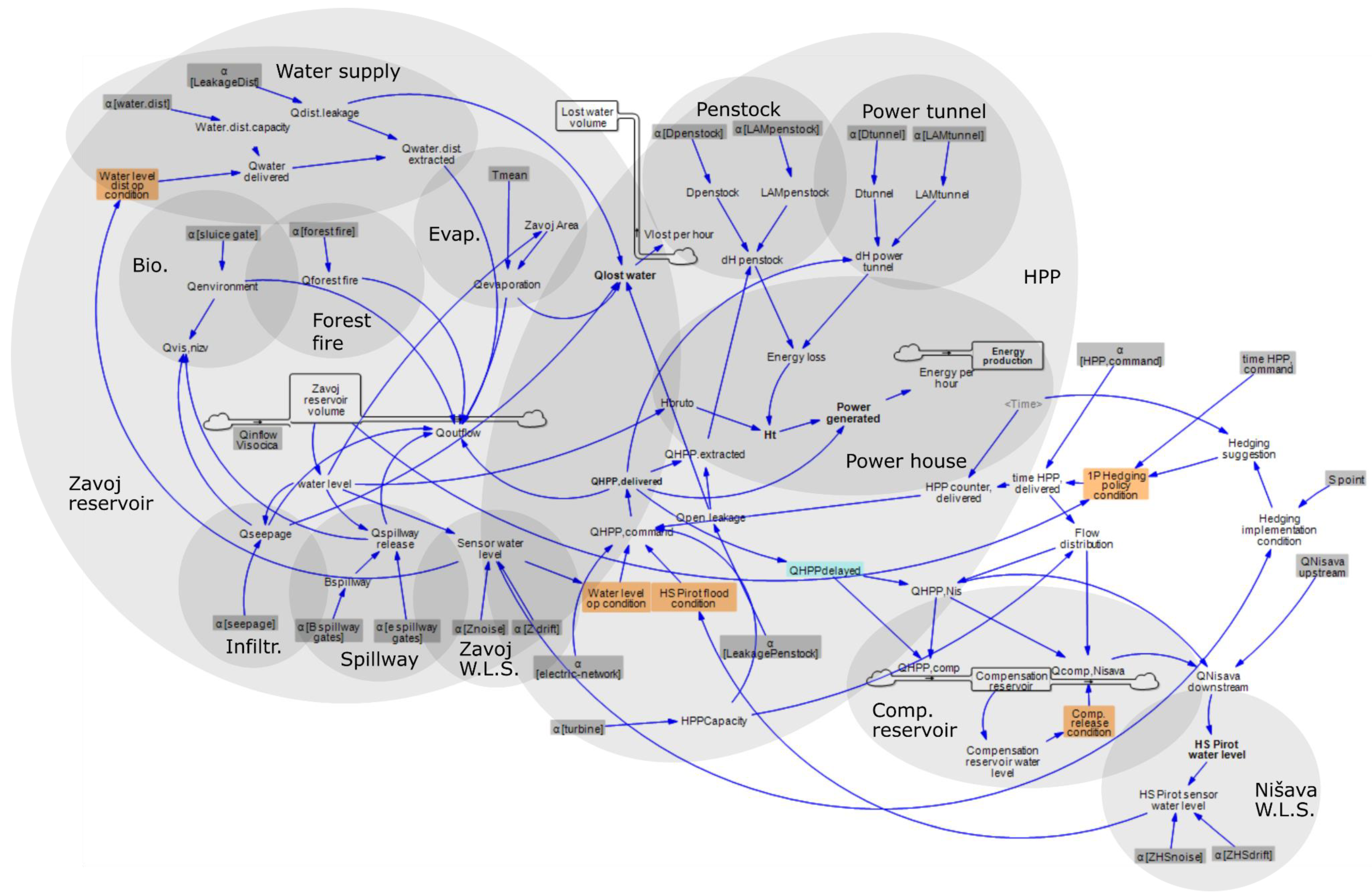
3.1. Pirot DRS Model Design

First, the decomposition of the system (Step 1, Figure 1) is performed. Key subsystem components, with appropriate interdependence links (Step 2), are presented in Figure 5. The system is decomposed in one of the many possible ways, with subsystems describing interactions of the physical system components with inputs, as well as the processes of interest for the water mass balance. In general, the decomposition step is deemed as a support for the conceptualization of the system, providing ground for the SD model design. Here, for example, more complex subsystems (on higher hierarchical levels), such as the Zavoj Reservoir, are represented by elements on lower hierarchical levels (simpler subsystems) which correspond to processes of interest and model a certain input/output transformation (Zavoj water-level sensors, spillway, biological outflow, infiltration, etc.). Some subsystems (e.g., power tunnel) are shared between two bigger subsystems (e.g., Zavoj Reservoir and HPP). It is evident that these subsystems can be decomposed further in lower hierarchical levels, with more details describing the ongoing process and causes, if it is deemed necessary.

To allow for the analysis of the Pirot DRS hydropower generation and flood protection, the mathematical representations of the subsystems, with a sufficient level of detail, are devised in Step 3. The storage elements, such as the Zavoj Reservoir and the compensation reservoir, are represented with the balance equation (Equation (2)), the total outflow towards HPP with Equation (3), the gated underflow with Equation (5), and the seepage outflow with Equation (6), while two level-monitoring points, in the Zavoj Reservoir and at the Nišava River, with Equation (7). Appropriate mathematical representation was used to calculate power tunnel and penstock head losses, needed to determine net turbine fall and later turbine power and energy production in the powerhouse subsystem.

The operation of the DRS is, in general, a complex process where many local process variables are monitored, collected, and/or computed to support the decision-making process and definition of the system’s operating actions. Here, the HPP operation, water extraction (entering the power tunnel), and energy production (in the powerhouse), and flow routing through the tailrace and compensation reservoir, are controlled with simple operating rules (Step 4) integrated in the control subsystem. This subsystem is integrated at the various points in the model and is designated to parse the external demands for power generation (e.g., how much will the HPP operate during the day), and also to implement how the system actuators will affect the control variables in respect to the appropriate process variables. In the BM variant, the HPP will operate for the demanded number of hours if the monitored water level in Zavoj Reservoir $Z_{zavoj}$ is above min $Z_{zavoj,min}$ and below max $Z_{zavoj,max}$ value, and similarly, the water level at Nišava River $Z_{Nišava}$ is below the critical value $Z_{Nišava,f.d.}$ determined in respect to the city of Pirot’s flood defense program. However, in the MMOR and MMORS variants, a discrete, one-point hedging policy is implemented, which allows for the decreasing of future severe shortages [37]. This hedging policy uses one parameter, $S$, which determines the storage value, below which the delivered power will be scaled down in respect to the daily request. When the storage value is above $S$, the full daily request is met. The implementation of the 1p discrete hedging policy did not exert major modifications in the system-model-design block although more complex rules probably would. HPP outflow is routed through the tailrace $Q_{HPP,Nišava}$ and compensation reservoir $Q_{HPP,comp}$, where the compensation reservoir volume is used to attenuate the release in the Nišava River. Characteristic trigger values, or control parameters, are an important part of the control subsystem (e.g., the minimum reservoir water level for HPP operation), which can be tuned to optimize the DRS’s system performance. The definition of these parameters, along with the external demands, is a part of the input-scenario-generation block.

The SD model was designed in the Vensim^® environment [38] (Ventana systems, 2021, Harvard, MA, USA). In Figure 6, the graph of the SD model is shown, where most of the model elements are grouped in accordance with the corresponding subsystems, to illustrate the relation to the previous conceptual system decomposition (Figure 5). The above-mentioned mathematical expressions are integrated in appropriate model elements and used in each time-step to calculate the changes in the state and operation of the system. For example, the water balance in the Zavoj Reservoir, with inflow from the Visočica River, and HPP, biological, overflow, seepage, evaporation, and forest fire outflows, can mathematically be represented as shown in Equation (14):

$$V_{zavoj}^{t+∆t}=V_{zavoj}^t+∆t·\left(Q_{visočica}^t-Q_{out,HPP}^t-Q_{bio}^t-Q_E^t-Q_{of}^t-Q_{inf}^t-Q_{ff}^t-Q_{wd}^t\right)$$

(14)

In Equation (14), $V_{zavoj}^t·\left(V_{zavoj}^{t+∆t}\right)$ represents the Zavoj Reservoir water volume at time $t$·($t+∆t)$, $∆t$ represents simulation time-step, $Q_{ff}^t$ is the firefighting water extraction (above 0 only when severe forest fire disturbance is occurring), while $Q_{wd}^t$ is the drinking water extraction, used in the MMORS model variant. Reservoir water level $Z_{zavoj}^t$ is evaluated using the stage-storage curve. However, at a lower hierarchy level, each of the reservoir outputs is defined in a separate subsystem model, where the failure-indicative parameters are detected (Step 5) and corresponding failure functions are integrated (Step 6). In total, 17 + 2 (added in MMORS) failure functions are introduced in the Pirot DRS dynamic model as shown in

Table 3. List of the subsystems with identified failure-indicative parameters and examples of functionality indicator implementation in the Pirot DRS SD model.

Subsystem	Failure-Indicative Parameter	Failure Functions	Failure Functions Implementation	Adverse Scenario 1 (AS1)	Adverse Scenario 2 (AS2)
Biological	$Q_{bio}$	${\alpha }_{sluice.gate}$	$f\left({\alpha }_{sluice.gate}\right)·Q_{bio}$	(E1)	(E1)
Seepage	$k,Q_{seeepage}$	$1/{\alpha }_K$	Equation (12)	(E1, E2)	(E1, E2)
Spillway	$B,Q_{spillway}$	${\alpha }_B$	Equation (11)	(E1, E2)	(E1, E2)
Firefighting extraction	$Q_{ff}$	$1-{\alpha }_{ff}$	Equation (16)	(FF1, FF2)	(FF1, FF2)
Power tunnel	$D_{tun},H_T$	${\alpha }_{D,tun}$	Equation (17)
	${\lambda }_{tun},H_T$	$1/{\alpha }_{\lambda ,tun}$	Equation (17)
Penstock	$D_{pen},H_T$	${\alpha }_{D,pen}$	Equation (17)	(E1)	(E1)
	${\lambda }_{pen},H_T$	$1/{\alpha }_{\lambda ,pen}$	Equation (17)	(E1, E2)	(E1, E2)
	$Q_{pen.leak.}$	$1-{\alpha }_{pen.leak.}$	Equation (15)	(E1, E2)	(E1, E2)
Powerhouse	$Q_{HPP}^t$	${\alpha }_{HPP}$	Equation (15)	(F)	(F)
	$P_{HPP}^t$	${\alpha }_{el.net.}$	Equation (18)	(E2)	(E2)
Zavoj water-level sensor	$∆Z_{noise},Z$	$1/{\alpha }_{Zavoj,noise}$	Equation (13)
	$∆Z_{drift},Z$	$1-{\alpha }_{Zavoj,drift}$	Equation (13)	(WLSZD)	(WLSZD)
Nišava water-level sensor	$∆Z_{HS,noise},Z$	$1/{\alpha }_{HS,noise}$	Equation (13)
	$∆Z_{HS,drift},Z$	$1-{\alpha }_{HS,drift}$	Equation (13)
Maintenance unit	$t_{proc,ik},$$(i-$subsystem; k-failure)	$1/{\alpha }_{proc}$	$f\left({\alpha }_{proc}\right)·t_{proc}$		(GMC)
	$t_{r,ik}$$,(i-$subsystem; k-failure)	$1/{\alpha }_r$	$f\left({\alpha }_r\right)·t_r$		(GMC)
Water distribution extraction	$Q_{wd.}$	${\alpha }_{wd.gate.}$	$f\left({\alpha }_{wd.gate.}^t\right)·Q_{wd}$	* (E1, E2)	* (E1, E2)
	$Q_{wd.leak.}$	$1-{\alpha }_{wd.leak.}$	$f\left({\alpha }_{wd.leak.}^t\right)·Q_{wd.leak.}^t$	* (E1, E2)	* (E1, E2)

* MMORS variant.

, for most of the defined subsystems. (Some subsystems do not have failure-indicative parameters.)

Water transport towards the HPP is represented by reservoir outflow $Q_{out,HPP}^t$, which is modelled within an appropriate subsystem model. In each step, the value $Q_{out,HPP}^t$ is calculated as:

$$Q_{out,HPP}^t=\underset{Q_{HPP}^t}{\underbrace{HPP,O{P}^t·{\alpha }_{HPP}^t·Q_{HPP,capacity}}}+\left(1-{\alpha }_{pen.leak.}^t\right)Q_{pen.leak.}^t$$

(15)

where $HPP,O{P}^t$ is a binary operator determining the command to operate or stand by, ${\alpha }_{HPP}^t$ is the functionality indicator used to demonstrate failure potential for turbine operation (e.g., one turbine is operational and the other is nonoperational due to main inlet valve failure ${\alpha }_{HPP}^t=0.5$), $Q_{HPP,capacity}$ is the total HPP capacity, ${\alpha }_{pen.leak.}^t$ is the penstock leakage functionality indicator, and $Q_{pen.leak.}^t$ is the estimated maximum value of leakage (e.g., failure-indicative parameter determined through the analysis of penstock material, current state, hydraulic conditions, etc.). In the model presented here, only penstock leakage is considered (enveloping leakage at the penstock and main inlet valve) although power tunnel leakage is also possible. Environmental outflow $Q_{bio}^t$ (and its failure potential related to the sluice gate operation) is simulated similarly as in Equation (15), while the evaporation $Q_E^t$ is modelled using an input temperature time-series [39]. Spillway underflow $Q_s^t$ is represented with an underflow/orifice Equation (11), while seepage is represented as in Equation (12). Fire-extinguishing outflow is added to simulate one of the effects of the forest fire disturbance:

$$Q_{ff}^t=\left(1-{\alpha }_{ff}\right)·Q_{ff,max}$$

(16)

where ${\alpha }_{ff}$ is introduced to represent the magnitude of water extraction for fire-extinguishing, and $Q_{ff,max}$ is estimated to be 0.15 m³/s. Power generated by the turbines $P_{HPP}^t$ at a specific time is evaluated using the following equations:

$$H_T^t=Z_{zavoj}^t-Z_{tr,HPP}^t-\frac{8·\raisebox{1ex}{${\lambda }_{tun}$}\!\left/ \!\raisebox{-1ex}{${\alpha }_{\lambda ,tun}^t$}\right.·L_{tun}}{{\left({\alpha }_{D,tun}^t·D_{tun}\right)}^5·{\pi }^2}·Q_{out,HPP}^t{}^2-\frac{8·\raisebox{1ex}{${\lambda }_{pen}$}\!\left/ \!\raisebox{-1ex}{${\alpha }_{\lambda ,pen}^t$}\right.·L_{pen}}{{\left({\alpha }_{D,pen}^t·D_{pen}\right)}^5·{\pi }^2}·\frac{Q_{out,HPP}^t{}^2}{2}$$

(17)

$$P_{HPP}^t={\alpha }_{el.net.}^t·\underset{P_{cap.HPP}^t}{\underbrace{{\eta }_T·\rho ·g·Q_{HPP}^t·H_T^t}}$$

(18)

where the $H_T^t$ is the turbine net fall, $Z_{tr,HPP}^t$ is the water level at the tailrace, and the values with subscript $tun$ and $pen$ are related to the power tunnel and penstock, respectively. The $P_{HPP}^t$ is generated power at the powerhouse, $P_{cap.HPP}^t$ is the capacity for power generation and ${\alpha }_{el.net.}^t$ is the functionality indicator used to model the disconnection of the HPP from the grid. Furthermore, two water-level monitoring systems are modelled as shown in Equation (13), at the Zavoj Reservoir and at the Nišava River (HS Pirot), where both monitored levels are used as process variables for the HPP operation control.

In the MMORS model variant, a new subsystem is included, representing the intake and transport of drinking water. It is described as a part of the Zavoj Reservoir subsystem, with a link to the storage reservoir (Figure 5). Two failure-indicative parameters are identified, $Q_{wd.}$ and $Q_{wd.leak.}$, which can model the reduction of the transport capacity and the increase of the water leakage within the transport infrastructure.

The maintenance subsystem in the used model variants serves solely to control the procurement and repair times for the identified failure-indicative parameters, affected by the disturbance scenarios. As will be shown in the next subsection, a global market crisis disturbance in one of the examined scenarios (AS2) will increase the procurement times (e.g., a failure-indicative parameter in maintenance subsystem) for mechanical spare parts, which is modelled with the simple failure function $f\left({\alpha }_{proc}\right)$, as shown in Table 3.

3.2. Input Scenario Generation for Pirot DRS

The generation of the input scenarios covers three distinct steps, as defined in Figure 1: Step 7: Hydrologic modelling and input time-series generation, Step 8: Definition of external demands and characteristic control parameters, and Step 9: Disturbance (failure) scenario generation. As the focus of this paper is on the modelling of the system components’ partial failure and various disturbance impacts, the scenarios analyzed here for the presented Pirot DRS dynamic model utilize the same set of the hydrometeorological input data throughout the simulations. Synthetic time series, based on the historical time-series from several hydrological and meteorological stations, were determined for inflow from the Visočica River into the Zavoj Reservoir $Q_{visočica}^t$, flow in the Nišava River at the hydrological station Pirot $Q_{Nišava}^t$, and air temperature needed for evaporation modelling ($Q_E^t$). More details regarding this modelling step can be found in [34].

The DRS operation is controlled and synchronized with the wider energy production, flood protection, environmental, and other management systems. In the simplified DRS dynamic model used here, the external requests for power generation (Step 7) are parsed through the Control subsystem. It is assumed that the external energy agency issues the daily request in terms of the number of HPP operating hours (here a constant demand of 10 operating hours during peak consumption is used), which may or may not be met, depending on the monitored data from the Zavoj Reservoir $Z_{zavoj}$ and Nišava River $Z_{Nišava}$. Control parameters, namely the characteristic trigger values $Z_{zavoj,min}$, $Z_{zavoj,max}$, $Z_{Nišava,f.d.}$, and $S$ are also defined here. The hedging policy parameter $S$ is optimized to maximize the energy production in the analyzed period.

Finally, the disturbance scenarios should be defined to complete the input scenario-generation block (Step 9). It should be highlighted that endogenous and exogeneous disturbances, such as earthquakes, material deterioration, etc., are defined within this step. Out-of-design range inflows can also be exogenous disturbances for a DRS but should be defined earlier in Step 6. The disturbances governed by Step 8 are represented through functionality indicators $\alpha$ time-series for each previously defined failure-indicative parameter and corresponding failure function. Naturally, the timing, magnitude, and duration of the disturbance play an important role, particularly when they coincide with extreme hydrological inputs. Here, the same set of inflows, as shown in Figure 6, was used in all of the simulations, with an extreme hydrological event in the form of the high inflow $Q_{visočica}^t$ occurring during the spring of the first year. Regarding disturbances, in the RS scenario (Table 2), all the $\alpha$ time-series have a constant value of 1, indicating that all the subsystems are in usual operation (Equation (10)). However, in the AS1 scenario, randomly chosen additional disturbances are introduced: two subsequent earthquakes, two forest fires, water-level sensor zero-drift (creeping drift up to 10 cm), and freezing at the power tunnel intake. These disturbances were arbitrarily chosen to demonstrate the implementation of the failure rates using the functionality indicator time-series It should be mentioned that a more realistic failure generator should use expert knowledge, previous events, and experience from similar objects, and finally envelop the probabilistic nature of the events. In this research, the main focus is on failure rate implementation, while disturbance event generation will be addressed in a separate investigation. Earthquakes hypothetically damage the sluice gate (reducing the biological outflow), increasing seepage, reducing the spillway capacity [21], damaging the penstock, and in the MMORS variant, the water-supply intake. The forest fires result in an increase in the water extraction for the firefighting, while freezing reduces the capacity of the power tunnel intake, leading to a lower turbine flow capacity. Furthermore, the AS2 scenario considers the same set of disturbances with the addition of a global market crisis affecting the maintenance subsystem, i.e., the time needed for the procurement of spare parts used to repair the mechanical system components (gates and turbines). Table 3 shows which of the functionality indicators have changed values due to the additional disturbances in scenarios AS1 and AS2. The combined input time-series defined in Steps 7–9 is illustrated in Figure 7. Figure 7b,c presents the functionality indicator time-series for AS1 and AS2, respectively, where the values of the indicators listed in Table 3 are varied during the time in respect to the modelled disturbances.

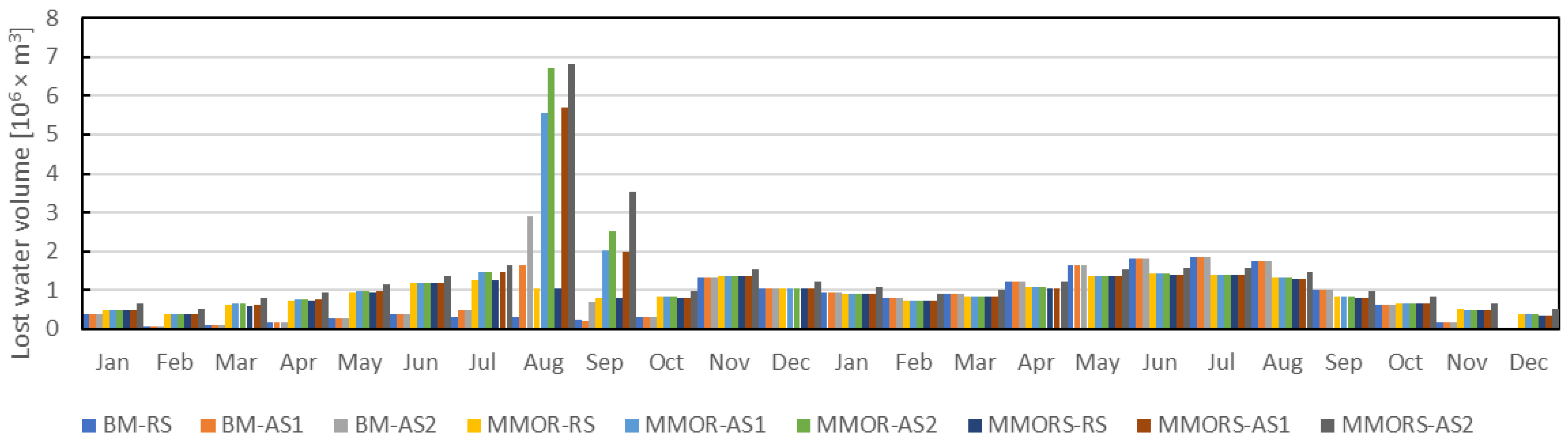
3.3. System Performance in Adverse Operating Conditions

Following the simulation of the Pirot DRS’s behavior (for each model variant) in the analyzed scenarios, a basic comparison can be performed. In the MMOR and MMORS variant, a 1p discrete hedging policy was used, yielding improved water deficiency distribution over BM, as expected. The total energy production is roughly the same, as is the total volume of the lost water (deviations up to 0.5%), but the water volume deficit between the beginning and the end of the simulation is reduced by 45%. The monthly values of generated energy and lost water are shown in Figure 8 and Figure 9, respectively. Total energy production decreases slightly with the introduction of the additional disturbances in AS1 and AS2 (up to 0.7%), mainly due to the increase in the water losses (leakages). In the months where the functionality of the HPP subsystems was reduced, such as after the freezing and earthquake disturbance, the production was lower although the large storage capacity of the Zavoj Reservoir allowed for the redistribution of the HPP production after the appropriate subsystems were repaired. However, the water loss increased significantly in AS1 and AS2, up to 57.8% in MMORS where the additional $Q_{wd.leak.}$ component was introduced. In absolute values, the increase of the water losses in the analyzed period was up to 8.39 × 10⁶ m³, which can be used to estimate the potential loss of the energy production (if a median turbine net fail $H_T$ is used) of up to 4.69 GWh. Using the EU average price of 0.219 €/kWh [40] this potential loss amounts to roughly ~1,000,000 €, highlighting the importance of more accurate failure modeling in the DRS operation analysis.

Disturbances primarily affect the capacity of the system to perform its intended functionalities. Here, besides hydropower generation, three more functions of the system are analyzed: the flood protection of the city of Pirot, the biological stability of the Visočica River, and the drinking water supply. Throughout the simulation periods, the flood protection function was unchallenged as the HPP did not stop operation due to the excessive monitored water levels at HS Pirot (The contribution from the HPP to the Nišava River did not coincide with any major inflow). However, the capacity of the system to provide the biological (environmental) outflow needed for downstream natural habitats was reduced for a certain period after the earthquakes (e.g., the blockage of the sluice gate and repair) with a total undelivered water volume of 320,100 m³. Furthermore, in the MMORS variants, the failure of the intake main valve led to a deficit in the drinking water supply of 482,400 m³. The impact of the global market crisis simulated in the AS2 scenarios led to even higher values of undelivered water volumes, 527,500 m³ and 949,000 m³, for biological outflow and water supply, respectively. Here, the global market crisis tripled the procurement time for the mechanical subsystem repair, emphasizing the need to consider the dynamics of the spare part availability within the DRS’s management and operation.

4. Discussion

To improve the understanding of DRS behavior in adverse operating conditions, a framework for the SD modelling of the DRS’s reduced functionality is presented here. The suggested framework identifies 11 steps, where Steps 1–6 cover the system-model-design block, 7–9 the input-scenario-generation, 10 the modelling/simulation, and finally Step 11, the evaluation of system performance. The system-model-design block considers decomposition of the system into subsystems, where each subsystem models the dynamics of the process or an input/output transformation with a level of detail tailored to the modelling task. Hierarchical decomposition can be used, where the subsystems can be further decomposed into lower-level subsystems, to capture all the necessary interactions between the components. Here, an emphasis is placed on the novel steps considering the identification of the failure-indicative parameters and the definition and implementation of the failure functions in the subsystem dynamic models. Failure-indicative parameters allow for the dynamic modelling of the reduced functionality of the DRS’s subsystems and components, common for the DRS’s operation in the adverse conditions. Through suggested failure functions with a generic functionality indicator as a variable, spanning from 0 to 1, the values of the failure-indicative parameters are modified in simulations, to emulate the component failure impacts on the DRS’s operation. Reduced functionality of the component lasts throughout the disturbance and failure duration. Failure duration envelops the procurement time (until the fault is detected and spare parts used for repair are procured) and repair time, when functionality can drop to 0 if such activity is needed. The input-scenario-generation block is composed of Step 7: Hydrological modelling, Step 8: Definition of the external demands and control parameters, and Step 9: Disturbance scenario generation. These steps are discussed briefly, where the complexity of the possible disturbance scenarios and large number of disturbances and their combinations, is emphasized. However, it is highlighted that, although the failure functions with generic functionality indicator provide a modelling capability for a large range of potential failures, some failures related to human aspects, such as operational mistakes and command-chain problems, require additional attention and further improvements. The final steps, including the DRS dynamic model simulations and system performance evaluation can lead to the modification of the original model. When new subsystems are defined, or existing ones are modified/upgraded, all of the framework steps should be revisited to check whether new interdependency links can be defined, failure-indicative parameters identifieds, etc.

The Pirot DRS case study is used to illustrate the framework implementation in the SD modelling process for a simple analysis of the DRS’s capacity to operate in the adverse operating conditions. Used adverse scenarios (AS1 and AS2) encompass extreme hydrological events and disturbances, such as earthquakes, freezing, sensor drift, forest fires, and global market crises. Disturbances in AS1, through failure functions and functionality indicators, affected failure-indicative parameters, such as the spillway opening, turbine capacity, penstock leakage, water-level-measurement uncertainty, firefighting water extraction, etc. In AS2, a global market crisis disturbance was added, leading to an increase in the mechanical spare part procurement time, yielding longer periods of reduced functionality. The use of the suggested framework allowed for the simulation of the scenarios, where some subsystems experienced moderate damage, but not complete failure, due to the disturbance event. In the life cycle of DRS systems, these scenarios are relatively frequent; hence, they should be analyzed in detail to provide a basis for impact mitigation. For the AS1 and AS2 scenarios, the analysis revealed that the disturbances lead to significant increases in water loss. Furthermore, significant water volumes were not delivered for biological control and water supply. It is shown that selected component failures and their combinations can severely affect the capacity of the system to deliver its intended functionality, hence highlighting the need for system behavior analysis in adverse operating conditions. These results should supplement a holistic approach to the decision-making process and provide stakeholders with additional valuable information.

However, in the modelling process, inherent limitations concerning the use of human expert knowledge in failure-scenario generation and failure-indicative parameter values definition still present a challenge. Additional investigation is needed to address these aspects. The proposed framework should be used to guide the system model design and the generation of the input scenarios; however, it should be stressed that the framework itself does not provide the modeler with the solution for the modelling problem at hand. To devise a reliable SD model, it is of paramount importance that the experienced operators of the DRS are engaged along with the management, stakeholders, and experts from the different engineering, ecological, and sociological fields. Failure scenarios and the estimated impact on the system, including the time needed to detect and procure the material for repair, as well as the repair time, are essentially defined by human experts; hence, the modeler should be aware of the uncertainties in their quantification and deal with them in an adequate manner. This is deemed as the inherent drawback of the suggested systems approach, which should be controlled by the modeler to the best of their knowledge.

5. Conclusions

A plethora of system performance analyses can be conducted with a reliable SD model of the DRS. Clearly, DRSs are complex systems controlling various transformations and processes, where different things can “go wrong,” leading to partial component failure and the reduction of system functionality. This paper presents a generic, straight-forward framework for the modelling and analyzing of DRSs’ reduced functionality in adverse operation conditions. The suggested framework identifies 11 steps, where Steps 1–6 define the system-model-design block, 7–9 the input scenario generation, 10 the modelling/simulation, and finally Step 11 addresses the evaluation of the system’s performance. An attempt was made to increase the SD modelling capability in adverse operating conditions where a DRS is experiencing reduced functionality, by taking into consideration a DRS’s decomposition, identification of failure-indicative parameters, and implementation of the failure functions with generic functionality indicator spanning in range 0–1. The framework is tested on the Pirot DRS case study, where a simple SD model capable of emulating a DRS’s reduced functionality was devised, based on which, system performance in several operating scenarios, was compared. According to the results obtained in this research, the following conclusions can be derived:

• A Complex DRS model can be decomposed into subsystems, where each subsystem describes a certain process or input/output transformation and interaction with other subsystems. Depending on the SD modelling goals, different forms of hierarchical DRS decomposition can be applied with varying levels of detail;
• With the identification of the failure-indicative parameters, definition and implementation of failure functions using generic functionality indicator as a variable, a wide variety of DRS disturbances, and respective disturbance and failure dynamics, can be modelled (physical damage, increase of measurement uncertainty, procurement of the spare parts, etc.);
• The flexibility of the proposed approach allows for the further development of the failure functions and modes, which can be used in the DRS behavior analysis in adverse operating conditions;
• The suggested framework can serve as guide for DRS SD model design, input-scenario generation, performance simulation and posteriori model modifications. However, it does not provide a solution for the modelling task;
• The dependability of SD modelling in respect to human expert knowledge remains a challenge. The modeler should be able to quantify the uncertainties related to the quantification of the failure-related parameters and control them in the modelling process.

Based on the results and previous conclusions, the suggested framework shows its potential for the wide use of DRS performance assessments in adverse operating conditions. However, the full application of this framework requires further investigation on input-scenario generation. More realistically, a probabilistic failure generator is also needed for the better implementation of the link between various natural and anthropogenic disturbances and DRS functionality in adverse operating conditions, which will be the subject of forthcoming research.

References

1. DeNeale, S.T.; Baecher, G.B.; Stewart, K.M.; Smith, E.D.; Watson, D.B. Current State-of-Practice in Dam Safety Risk Assessment; (No. ORNL/TM-2019/1069); Oak Ridge National Lab. (ORNL): Oak Ridge, TN, USA, 2019. [Google Scholar]
2. Winz, I.; Brierley, G.; Trowsdale, S. The Use of System Dynamics Simulation in Water Resources Management. Water Resour. Manag. 2008, 23, 1301–1323. [Google Scholar] [CrossRef]
3. King, L.M.; Schardong, A.; Simonovic, S.P. A Combinatorial Procedure to Determine the Full Range of Potential Operating Scenarios for a Dam System. Water Resour. Manag. 2019, 33, 1451–1466. [Google Scholar] [CrossRef]
4. CDA (Canadian DamAssociation). Available online: https://cda.ca/dams-in-canada/dams-in-canada (accessed on 26 March 2022).
5. Fema, M. Federal Guidelines for Dam Safety Risk Management; Federal Emergency Management Agency: Washington, DC, USA, 2015. [Google Scholar]
6. Chernet, H.H.; Alfredsen, K.; Midttømme, G.H. Safety of Hydropower Dams in a Changing Climate. J. Hydrol. Eng. 2014, 19, 569–582. [Google Scholar] [CrossRef]
7. Li, W.; Li, Z.; Ge, W.; Wu, S. Risk Evaluation Model of Life Loss Caused by Dam-break Flood and Its Application. Water 2019, 11, 1359. [Google Scholar] [CrossRef] [Green Version]
8. Đorđević, B.; Dašić, T.; Plavšić, J. Uticaj klimatskih promena na vodoprivredu Srbije i mere koje treba preduzimati u cilju zaštite od negativnih uticaja (in Serbian). Vodoprivreda 2020, 52, 39–68. Available online: https://www.vodoprivreda.net/wp-content/uploads/2020/12/3-Djordjevic-Dasic-Plavsic.pdf (accessed on 26 March 2022).
9. Badr, A.; Yosri, A.; Hassini, S.; El-Dakhakhni, W. Coupled Continuous-Time Markov Chain–Bayesian Network Model for Dam Failure Risk Prediction. J. Infrastruct. Syst. 2021, 27, 04021041. [Google Scholar] [CrossRef]
10. Srivastava, A. A Computational Framework for Dam Safety Risk Assessment with Uncertainty Analysis. Ph.D. Thesis, Utah State University, Logan, UT, USA, 2013. [Google Scholar]
11. Nápoles, O.M.; Delgado-Hernández, D.J.; De-León-Escobedo, D.; Arteaga-Arcos, J.C. A continuous Bayesian network for earth damsߣ risk assessment: Methodology and quantification. Struct. Infrastruct. Eng. 2013, 10, 589–603. [Google Scholar] [CrossRef]
12. Delgado-Hernández, D.-J.; Nápoles, O.M.; De-León-Escobedo, D.; Arteaga-Arcos, J.C. A continuous Bayesian network for earth dams’ risk assessment: An application. Struct. Infrastruct. Eng. 2012, 10, 225–238. [Google Scholar] [CrossRef]
13. Hartford, D.N.; Baecher, G.B. Risk and Uncertainty in Dam Safety; Thomas Telford Ltd.: London, UK, 2004. [Google Scholar]
14. Jiang, J.P.; Yang, Z.H. Laws of dam failures of small-sized reservoirs and countermeasures. Chin. J. Geotech. Eng. 2008, 30, 1626–1631. [Google Scholar]
15. Zhang, L.; Xu, Y.; Jia, J. Analysis of earth dam failures: A database approach. Georisk: Assess. Manag. Risk Eng. Syst. Geohazards 2009, 3, 184–189. [Google Scholar] [CrossRef] [Green Version]
16. Cleary, P.; Prakash, M.; Mead, S.; Lemiale, V.; Robinson, G.K.; Ye, F.; Ouyang, S.; Tang, X. A scenario-based risk framework for determining consequences of different failure modes of earth dams. Nat. Hazards 2014, 75, 1489–1530. [Google Scholar] [CrossRef]
17. Andreini, M.; Gardoni, P.; Pagliara, S.; Sassu, M. Probabilistic Models for Erosion Parameters and Reliability Analysis of Earth Dams and Levees. ASCE-ASME J. Risk Uncertain. Eng. Syst. Part A Civ. Eng. 2016, 2, 04016006. [Google Scholar] [CrossRef]
18. Ribas, J.R.; Severo, J.C.R.; Guimarães, L.F.; Perpetuo, K.P.C. A fuzzy FMEA assessment of hydroelectric earth dam failure modes: A case study in Central Brazil. Energy Rep. 2021, 7, 4412–4424. [Google Scholar] [CrossRef]
19. King, L.M.; Simonovic, S.P.; Hartford, D.N.D. Using system dynamics simulation for assessment of hydropower system safety. Water Resour. Res. 2017, 53, 7148–7174. [Google Scholar] [CrossRef]
20. King, L.M. Using a Systems Approach to Analyze the Operational Safety of Dams. Ph.D. Thesis, University of Western Ontario, London, ON, Canada, 2020. [Google Scholar]
21. Rakić, D.; Stojković, M.; Ivetić, D.; Živković, M.; Milivojević, N. Failure Assessment of Embankment Dam Elements: Case Study of the Pirot Reservoir System. Appl. Sci. 2022, 12, 558. [Google Scholar] [CrossRef]
22. Stowasser, E. L Dam failure system modeling in the muskingum watershed—Beach City Dam. In Proceedings of the 31st Annual USSD Conference, San Diego, CA, USA, 11–15 April 2011. [Google Scholar]
23. Haimes, Y.Y.; Petrakian, R.; Karlsson, P.O.; Mitsiopoulos, J. Multiobjective Risk Partitioning: An Application to Dam Safety Risk Analysis; Environmental systems management, Inc.: Charlottesville, VA, USA, 1988. [Google Scholar]
24. Baecher, G.; Ascila, R.; Hartford, D.N.D. Hydropower and dam safety. In Proceedings of the STAMP/STPA Workshop, Cambridge, MA, USA, 26 March 2013. [Google Scholar]
25. Regan, P.J. Dams as systems-a holistic approach to dam safety. In Proceedings of the 30th Annual USSD Conference, Sacramento, CA, USA, 12–16 April 2010; pp. 554–563. [Google Scholar]
26. Leveson, N.G. Engineering a Safer World: Systems Thinking Applied to Safety; The MIT Press: Cambridge, MA, USA, 2011; p. 560. [Google Scholar]
27. Thomas, J.P., IV. Extending and Automating a Systems—Theoretic Hazard Analysis for Requirements Generation and Analysis. Ph.D. Thesis, Massachusetts Institute of Technology, Cambridge, MA, USA, 2013. [Google Scholar]
28. Komey, A.; Deng, Q.; Baecher, G.B.; Zielinski, P.A.; Atkinson, T. Systems reliability of flow control in dam safety. In Proceedings of the 12th International Conference on Application of Statistics and Probability in Civil Engineering, ICASP12, Vancouver, BC, Canada, 12–15 July 2015; pp. 1–8. [Google Scholar]
29. Komey, A. A Systems Reliability Approach to Flow Control in Dam Safety Risk Analysis. Ph.D. Thesis, University of Maryland, College Park, MD, USA, 2014. [Google Scholar]
30. Hartford, D.; Baecher, G.; Zielinski, P.; Patev, R. Operational Safety of Dams and Reservoirs—Understanding the Reliability of Flow-Control Systems; ICE Publishing: London, UK, 2016. [Google Scholar]
31. Simonovic, S.P.; Arunkumar, R. Comparison of static and dynamic resilience for a multipurpose reservoir operation. Water Resour. Res. 2016, 52, 8630–8649. [Google Scholar] [CrossRef]
32. Stojkovic, M.; Simonovic, S.P. System Dynamics Approach for Assessing the Behaviour of the Lim Reservoir System (Serbia) under Changing Climate Conditions. Water 2019, 11, 1620. [Google Scholar] [CrossRef] [Green Version]
33. Simonovic, S.P. Application of the Systems Approach to the Management of Complex Water Systems. Water 2020, 12, 2923. [Google Scholar] [CrossRef]
34. Ignjatović, L.; Stojković, M.; Ivetić, D.; Milašinović, M.; Milivojević, N. Quantifying Multi-Parameter Dynamic Resilience for Complex Reservoir Systems Using Failure Simulations: Case Study of the Pirot Reservoir System. Water 2021, 13, 3157. [Google Scholar] [CrossRef]
35. Hashimoto, T.; Stedinger, J.R.; Loucks, D.P. Reliability, resiliency, and vulnerability criteria for water resource system performance evaluation. Water Resour. Res. 1982, 18, 14–20. [Google Scholar] [CrossRef] [Green Version]
36. Behboudian, M.; Kerachian, R.; Pourmoghim, P. Evaluating the long-term resilience of water resources systems: Application of a generalized grade-based combination approach. Sci. Total Environ. 2021, 786, 147447. [Google Scholar] [CrossRef]
37. Tayebiyan, A.; Mohammad, T.A.; Al-Ansari, N.; Malakootian, M. Comparison of Optimal Hedging Policies for Hydropower Reservoir System Operation. Water 2019, 11, 121. [Google Scholar] [CrossRef] [Green Version]
38. Vensim-Ventana Systems Inc. Available online: https://vensim.com/docs/ (accessed on 26 March 2022).
39. Linacre, E.T. A simple formula for estimating evaporation rates in various climates, using temperature data alone. Agric. Meteorol. 1977, 18, 409–424. [Google Scholar] [CrossRef]
40. Eurostat-European Commission. Available online: https://ec.europa.eu/eurostat/statistics-explained/index.php?title=Electricity_price_statistics (accessed on 26 March 2022).
Figure 1. Schematic framework overview.
Water 14 01549 g001
Figure 2. Example of system decomposition and definition of the interdependence links.
Water 14 01549 g002
Figure 3. Example functionality indicator α time-series, representing generic failures in three elements due to the two disturbances.
Water 14 01549 g003
Figure 4. Schematic representation of the Pirot DRS.
Water 14 01549 g004
Figure 5. Conceptualization of the decomposed Pirot DRS with interdependency links between subsystems.
Water 14 01549 g005
Figure 6. Pirot DRS dynamic model representation using Vensim software with reference to the subsystems defined in Figure 5, for MMORS model variant.
Water 14 01549 g006
Figure 7. Input time-series: (a) Visočica and Nišava River inflows with Zavoj air temperatures; (b) functionality indicator time-series for AS1; (c) functionality indicator time-series for AS2.
Water 14 01549 g007
Figure 8. Energy production per month for each model variant and input scenario.
Water 14 01549 g008
Figure 9. Water volume loss per month for each model variant and input scenario.
Water 14 01549 g009