
A Novel Hybrid Approach Based on Cellular Automata and a Digital Elevation Model for Rapid Flood Assessment


Abstract
1. Introduction
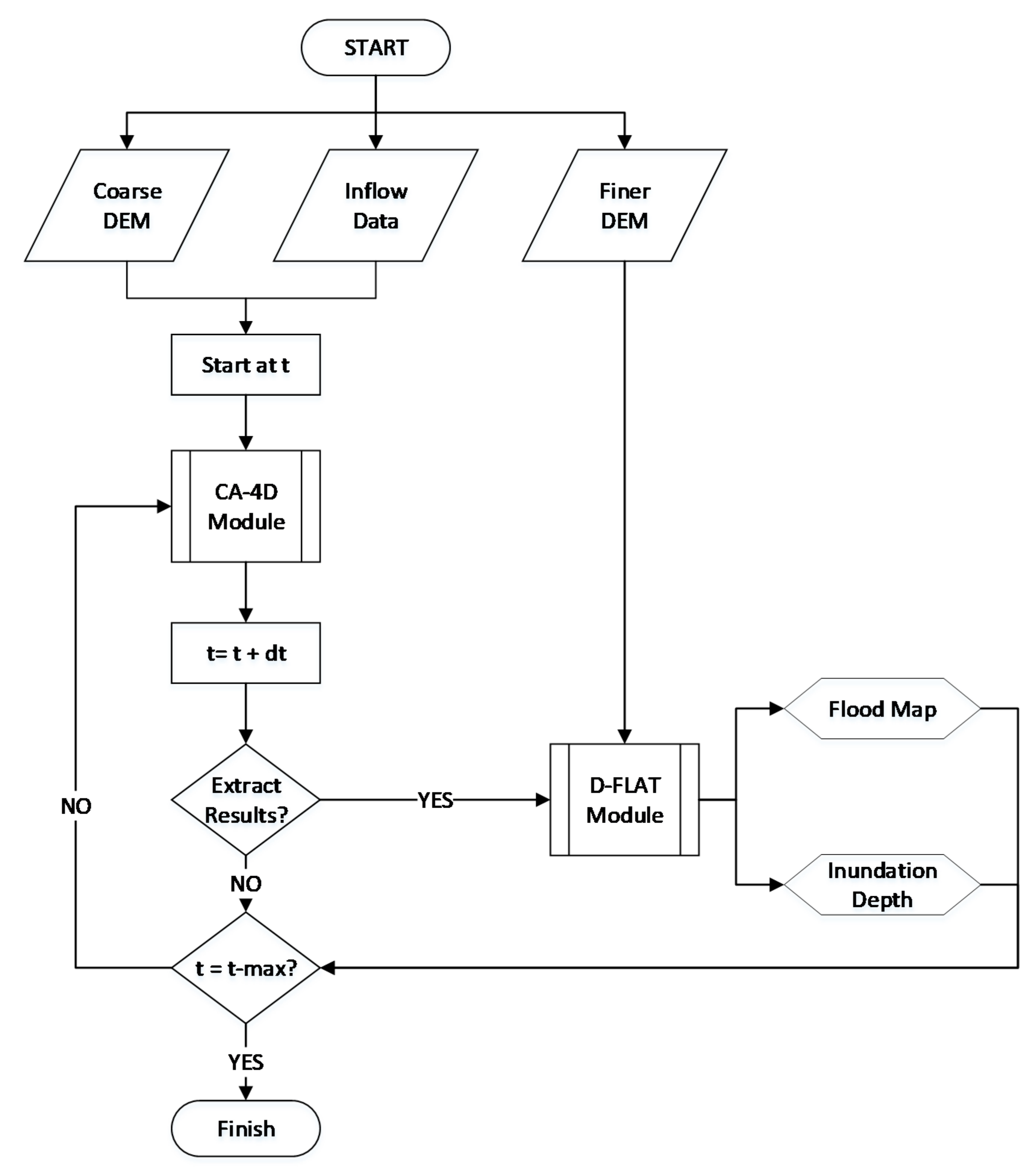
2. Hybrid Inundation Model
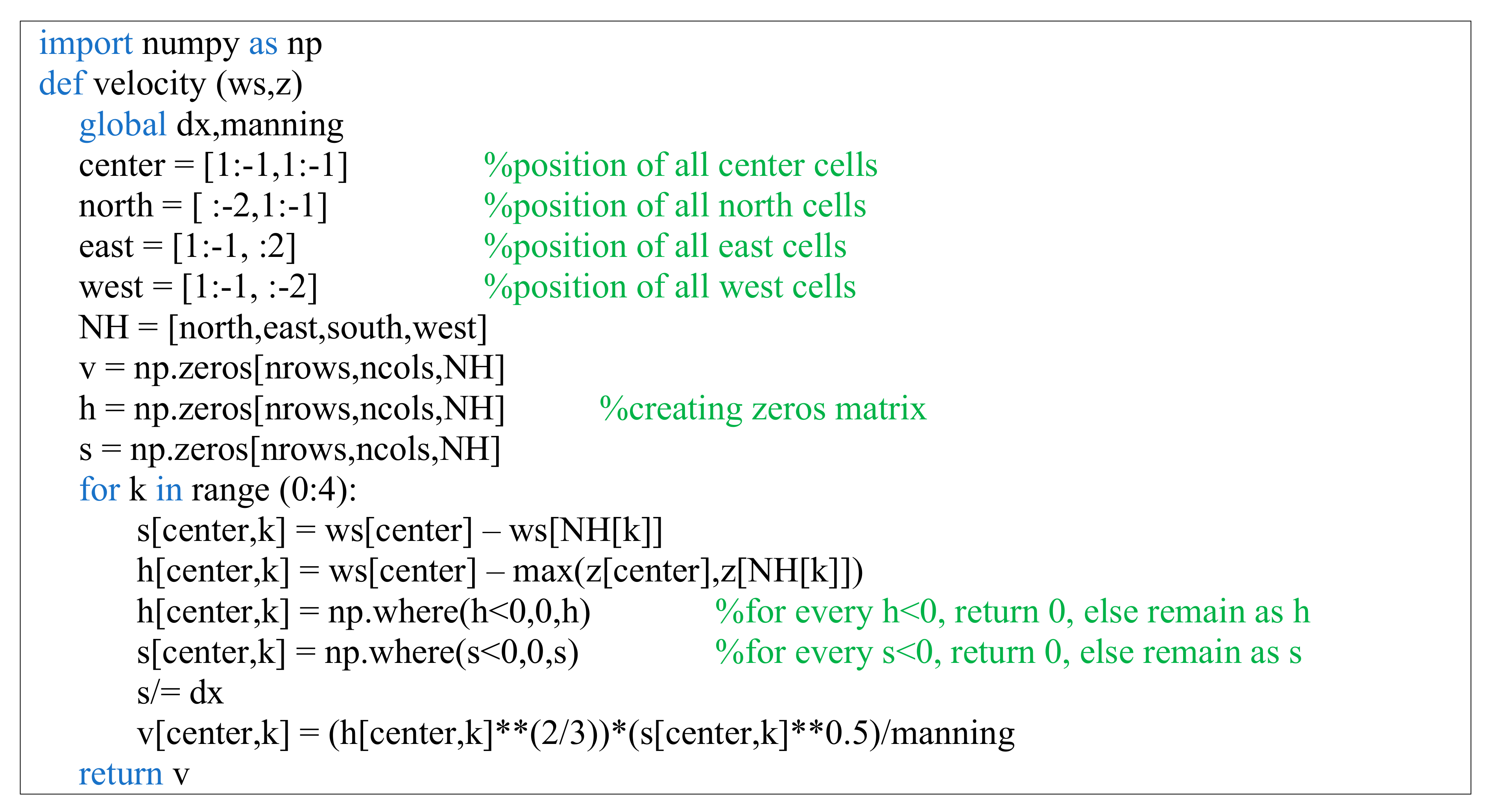
2.1. Cellular Automata 4-Direction (CA-4D) Model
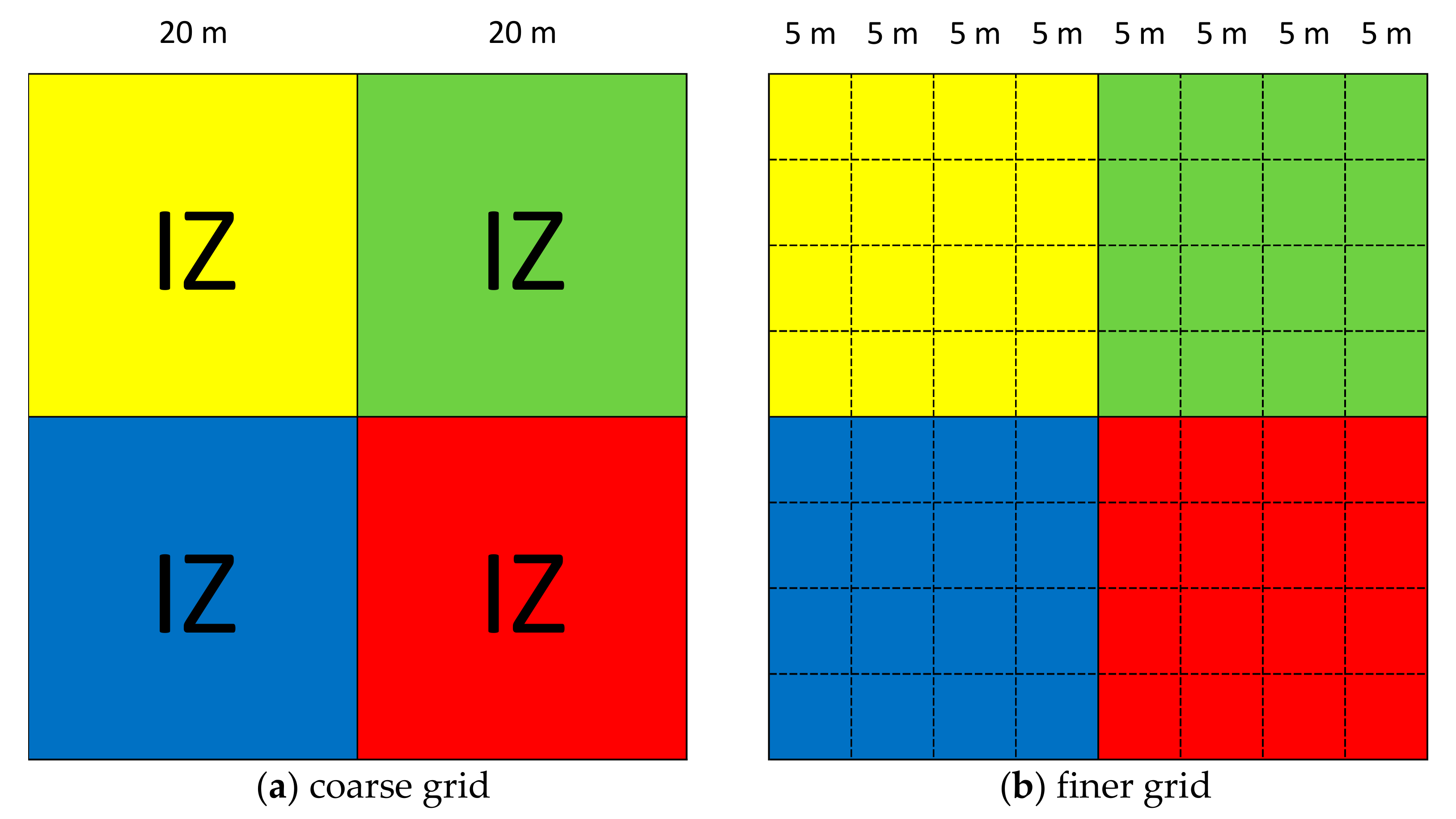
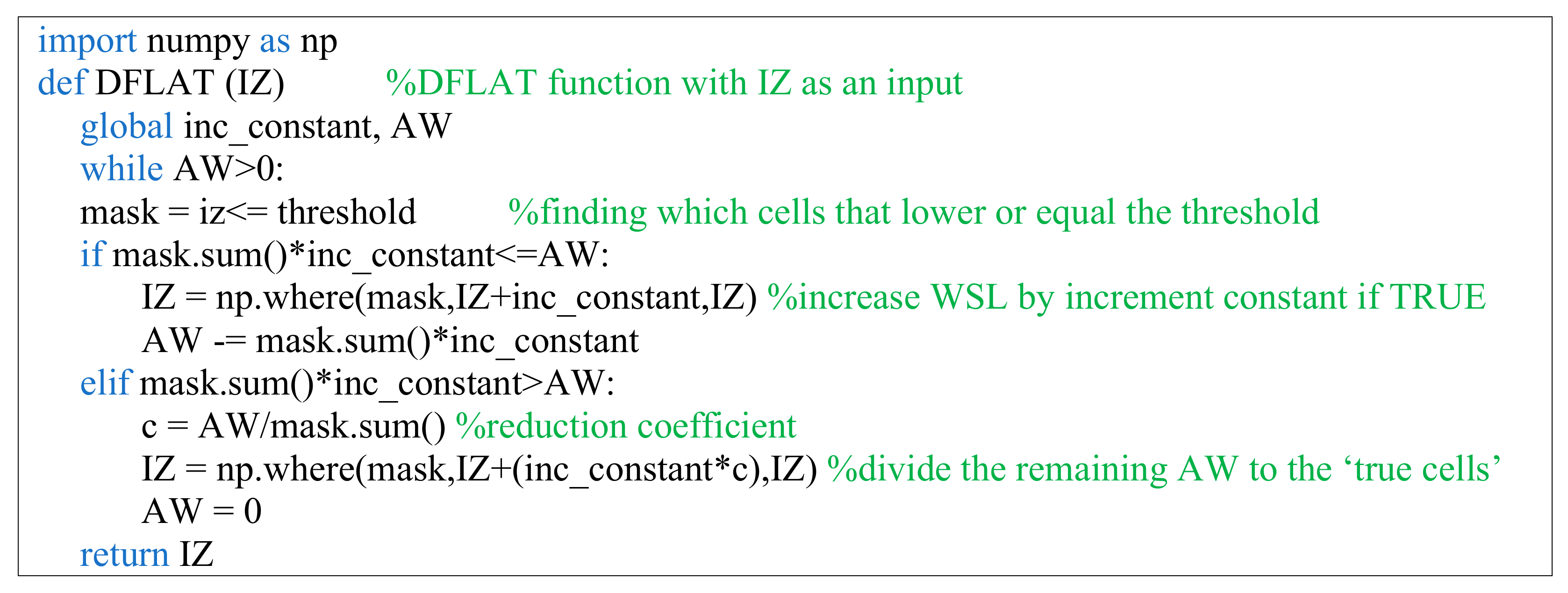
2.2. DEM Based on the Flat-Water Assumption (D-Flat) Model
3. Details of Case Studies
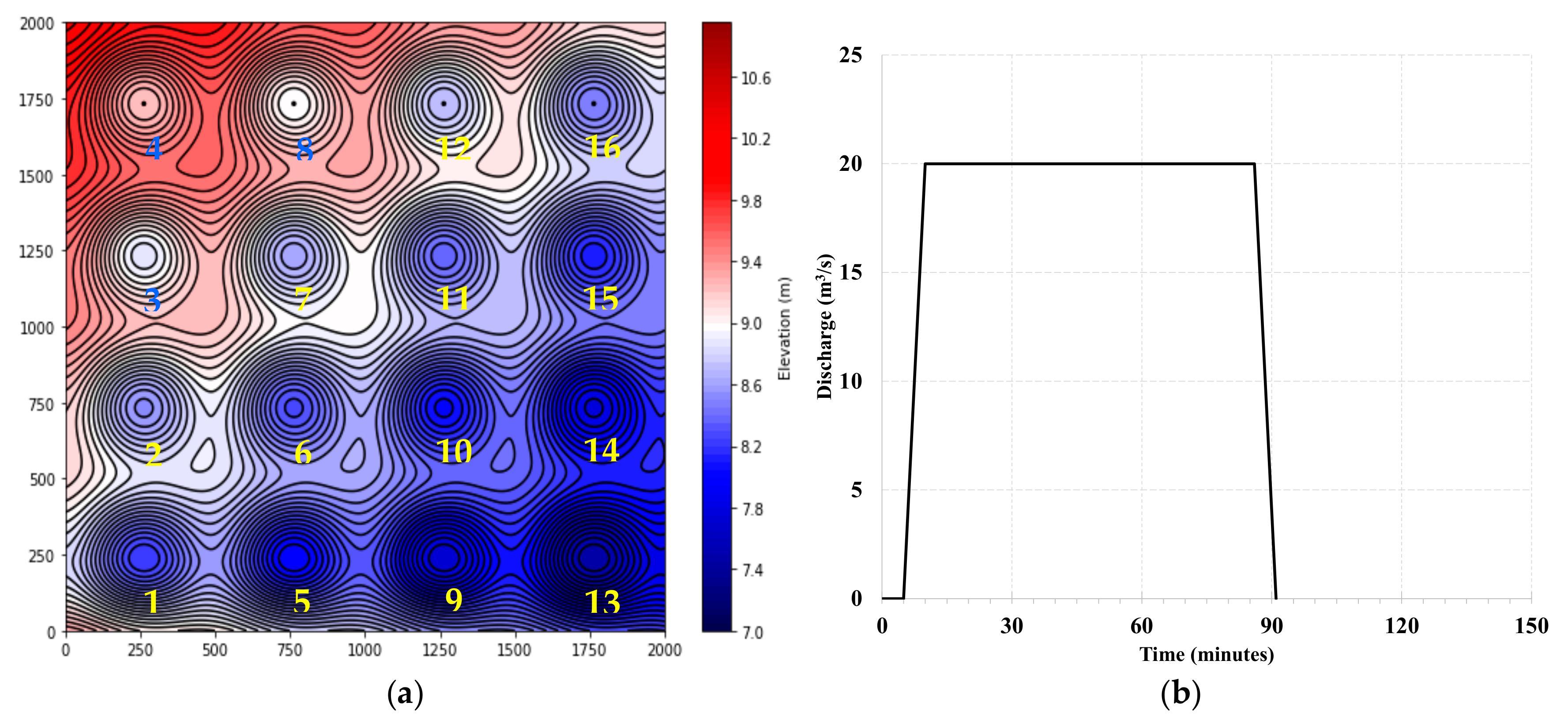
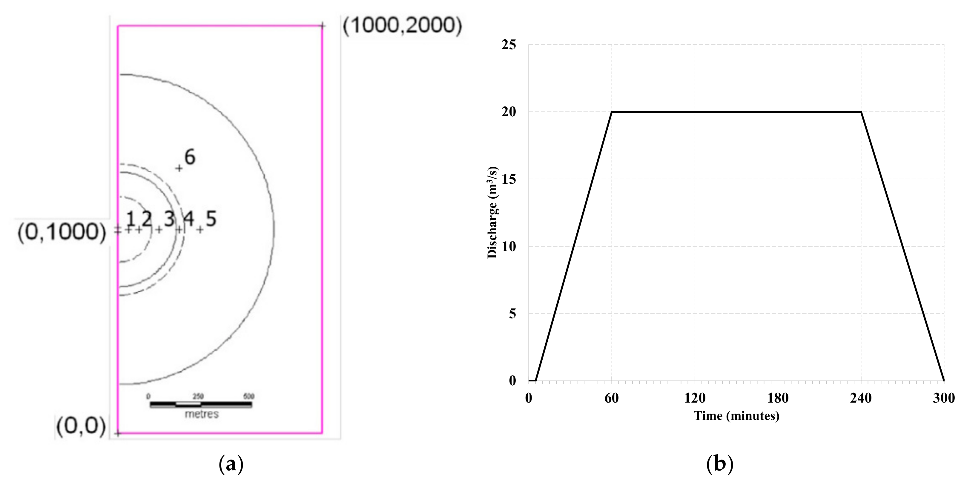
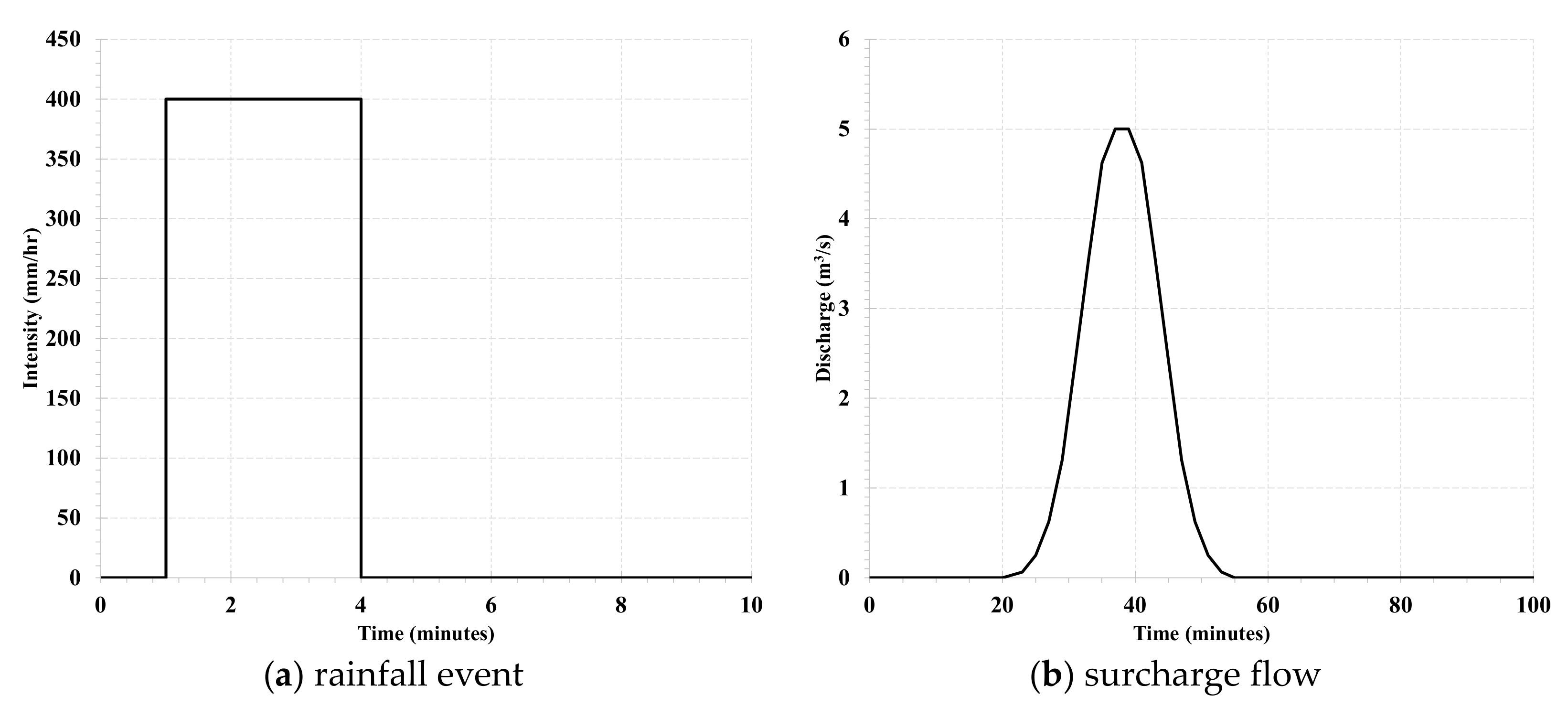
3.1. Three UK EA Benchmark Test Cases
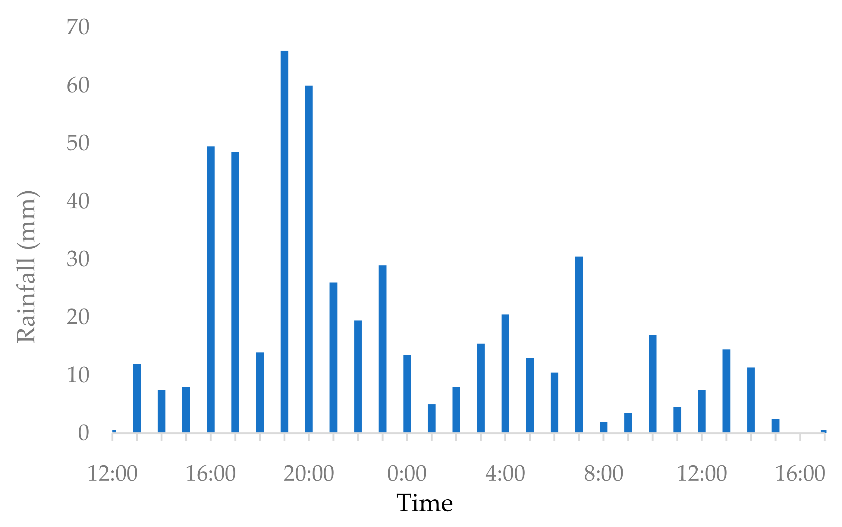
3.2. A Historical Flood Event
4. Results and Discussion
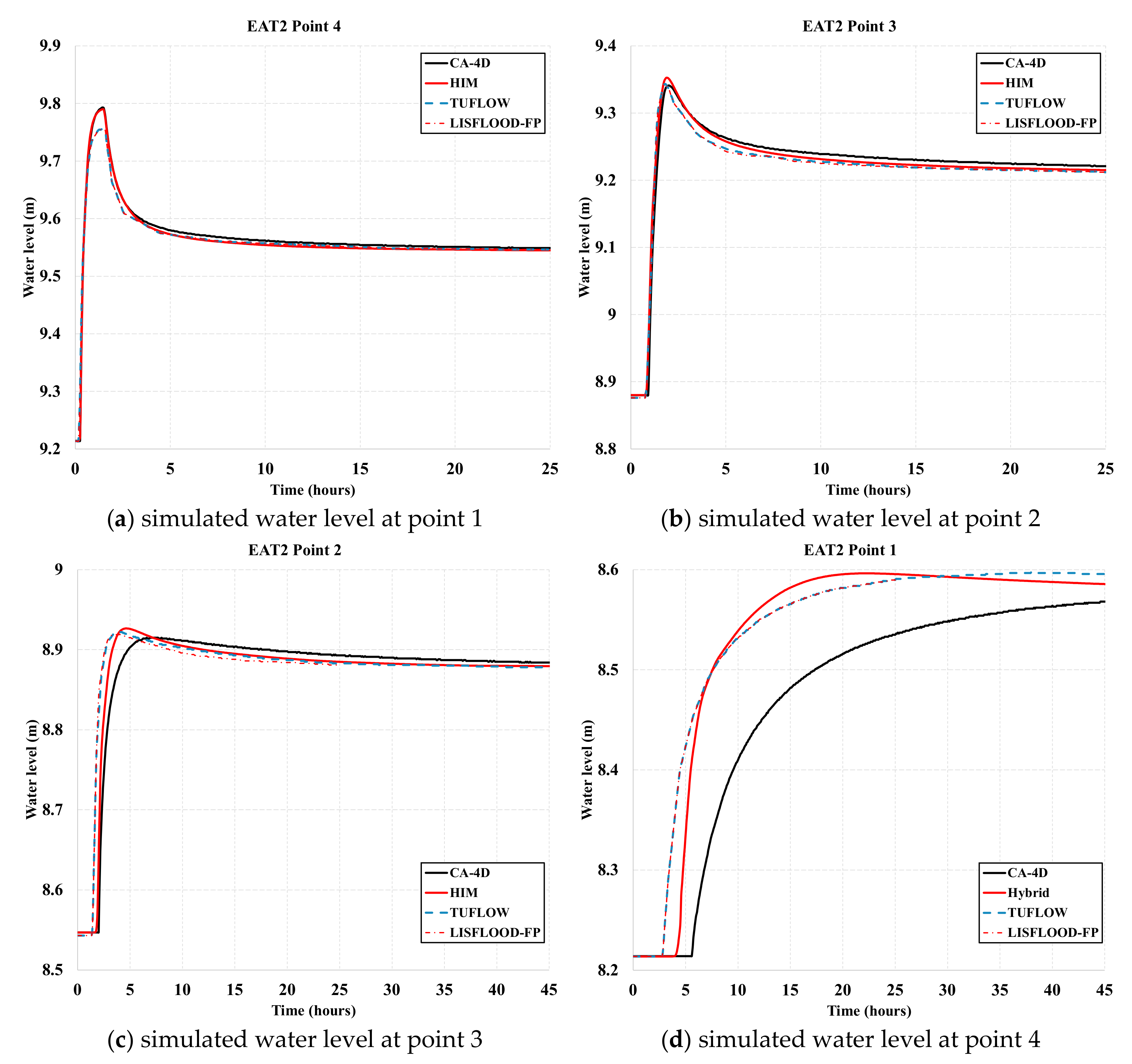
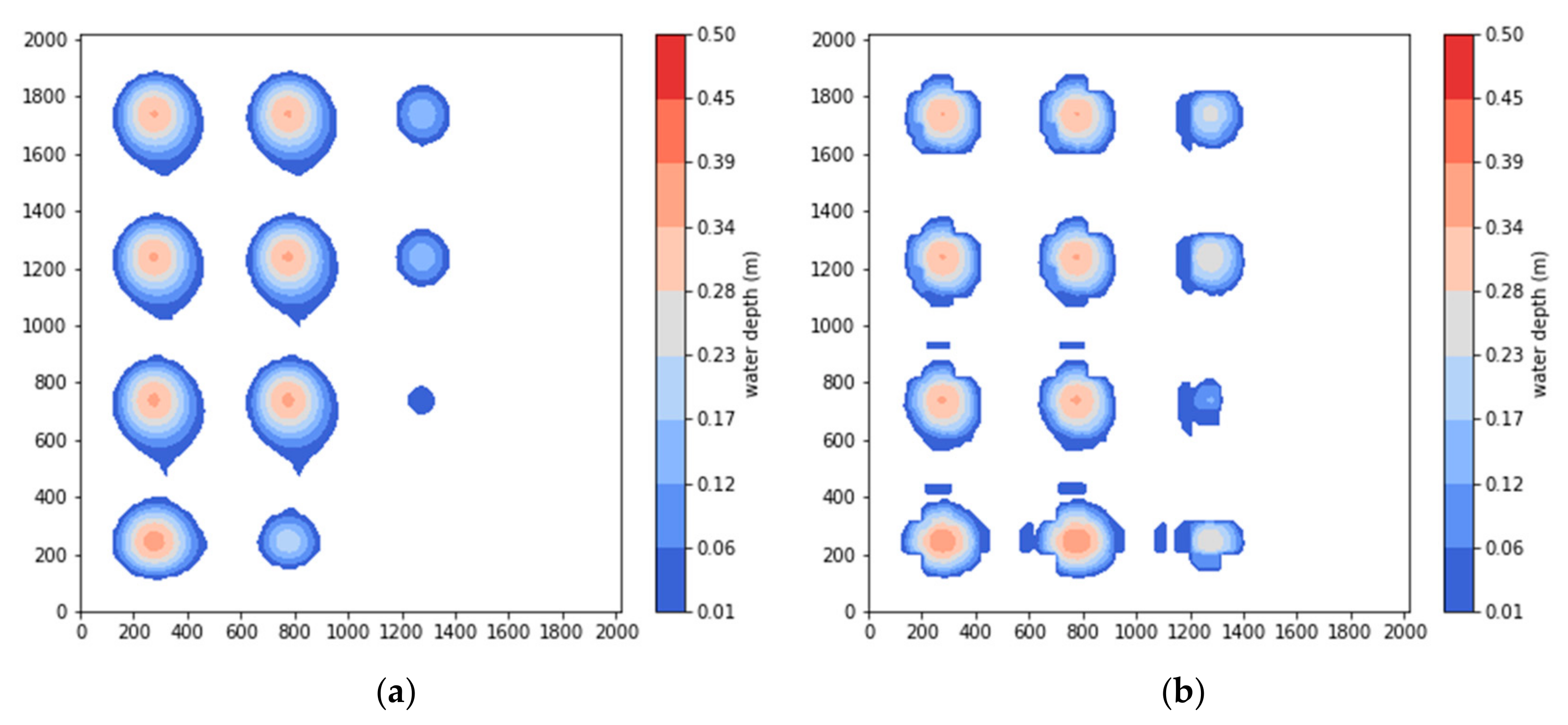
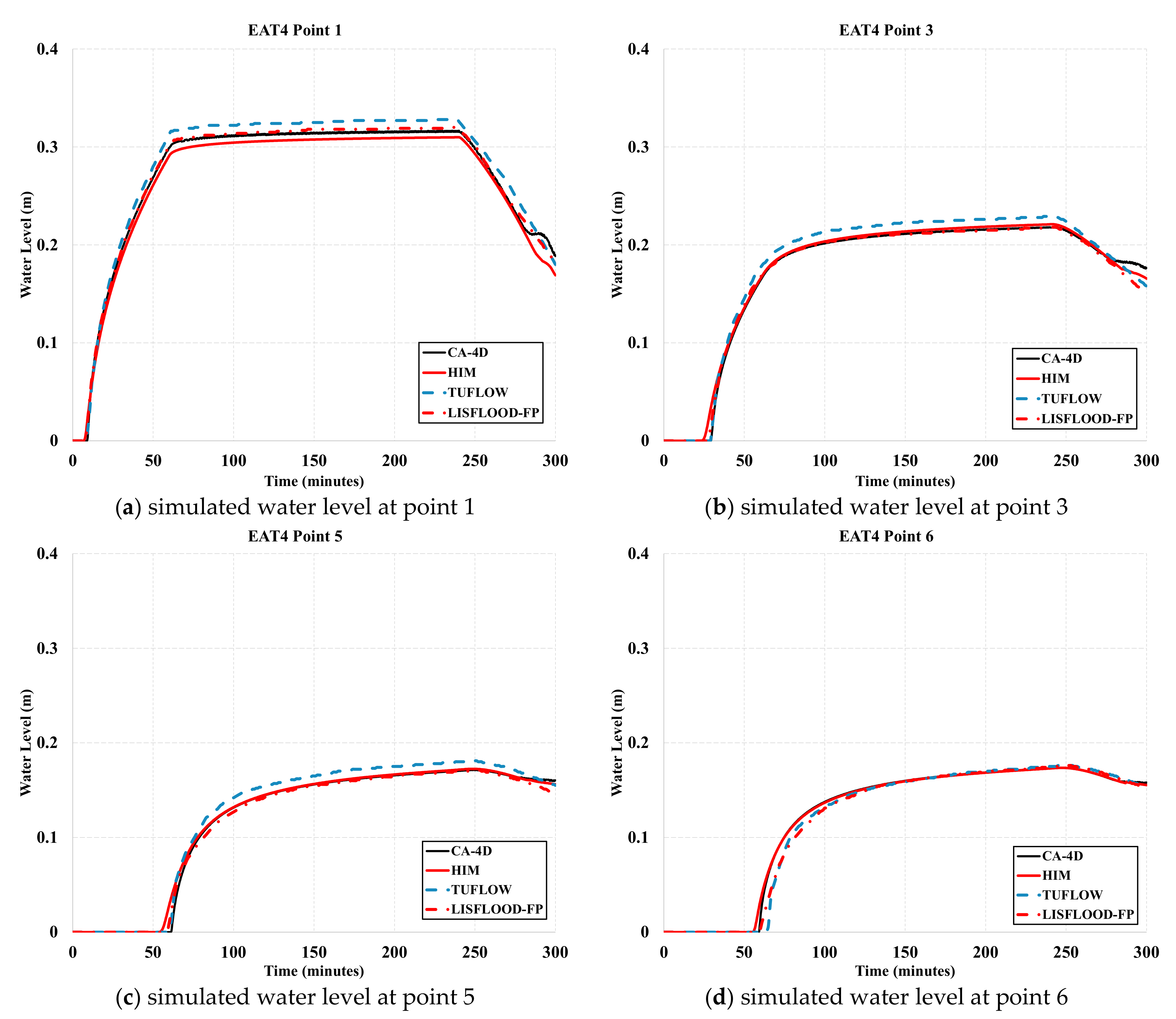
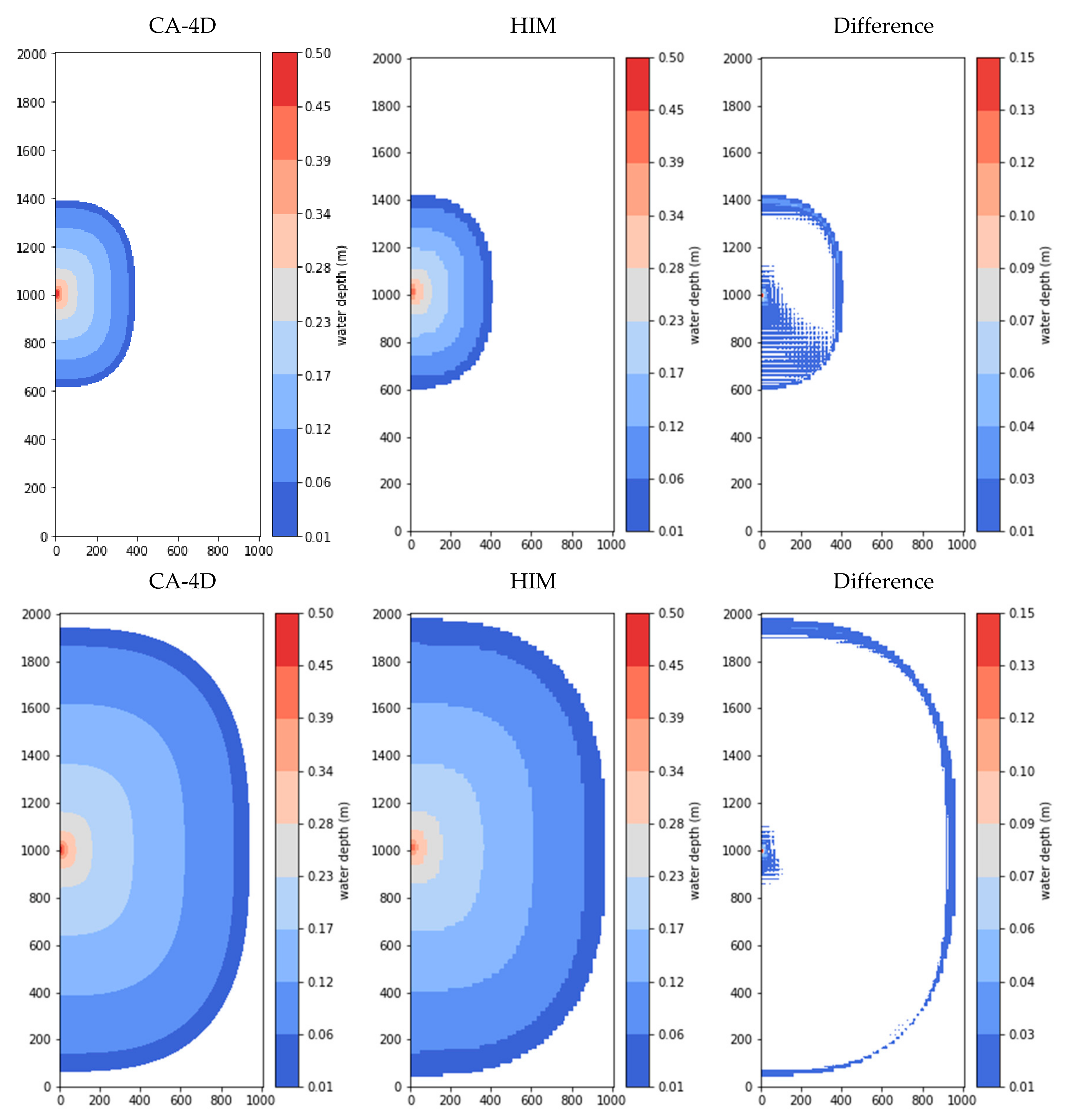
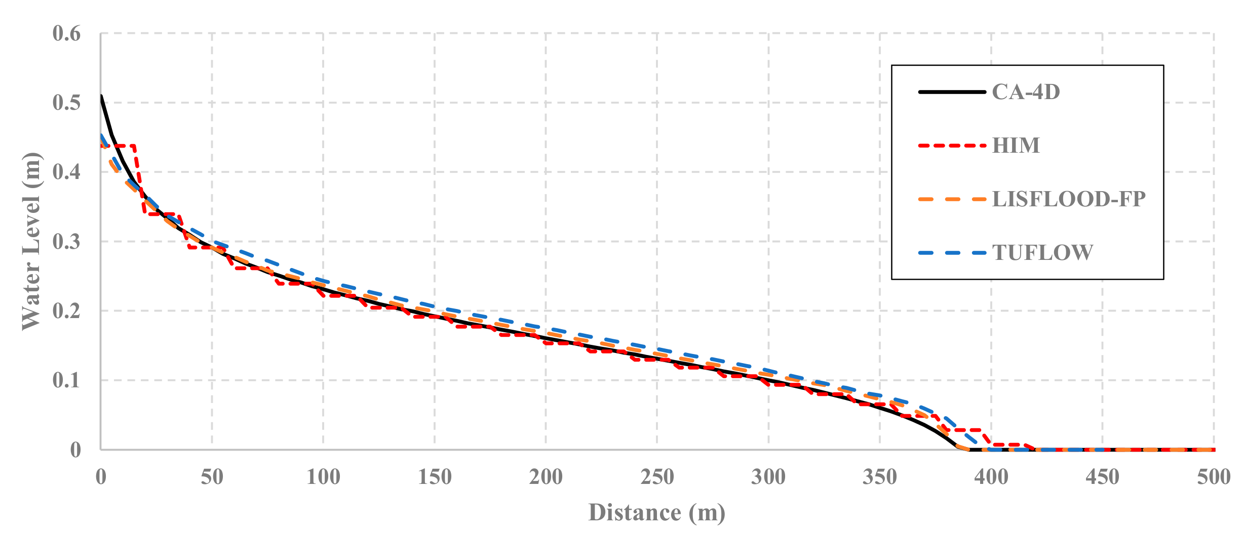
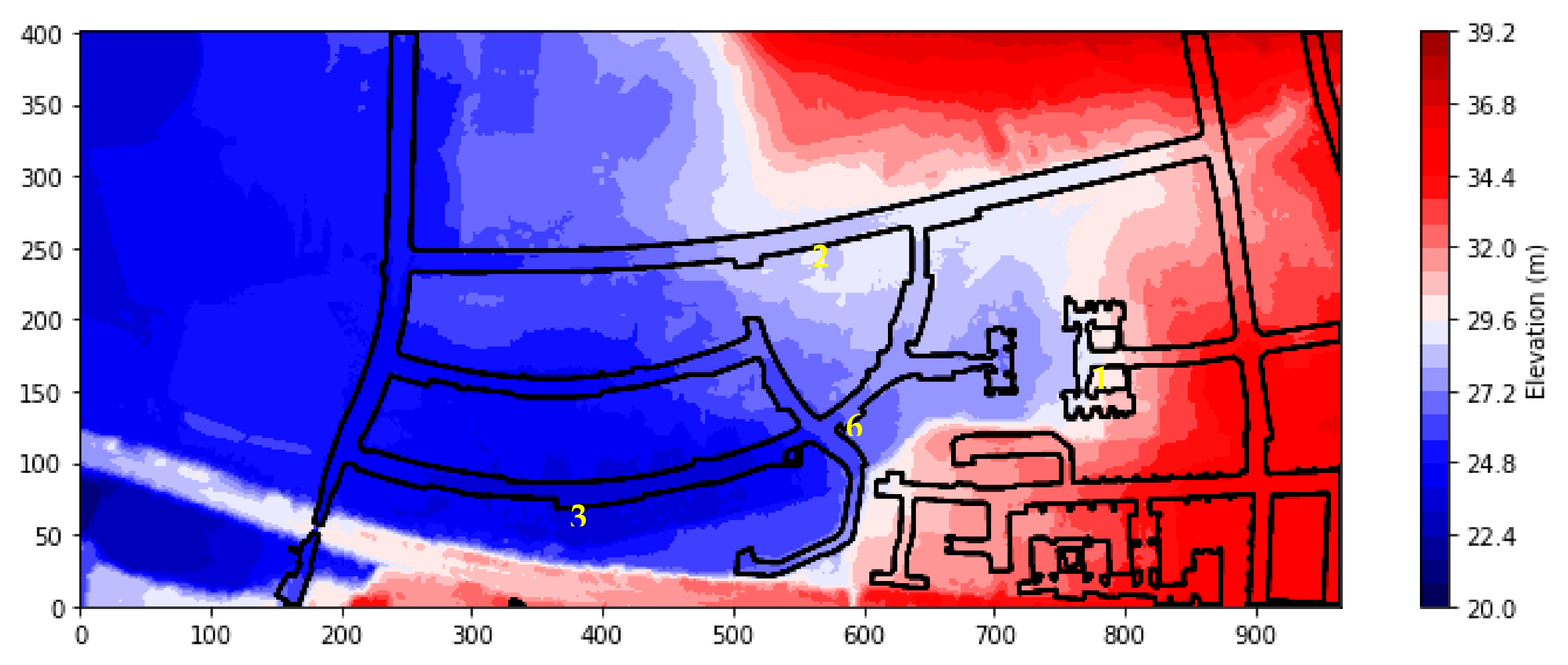
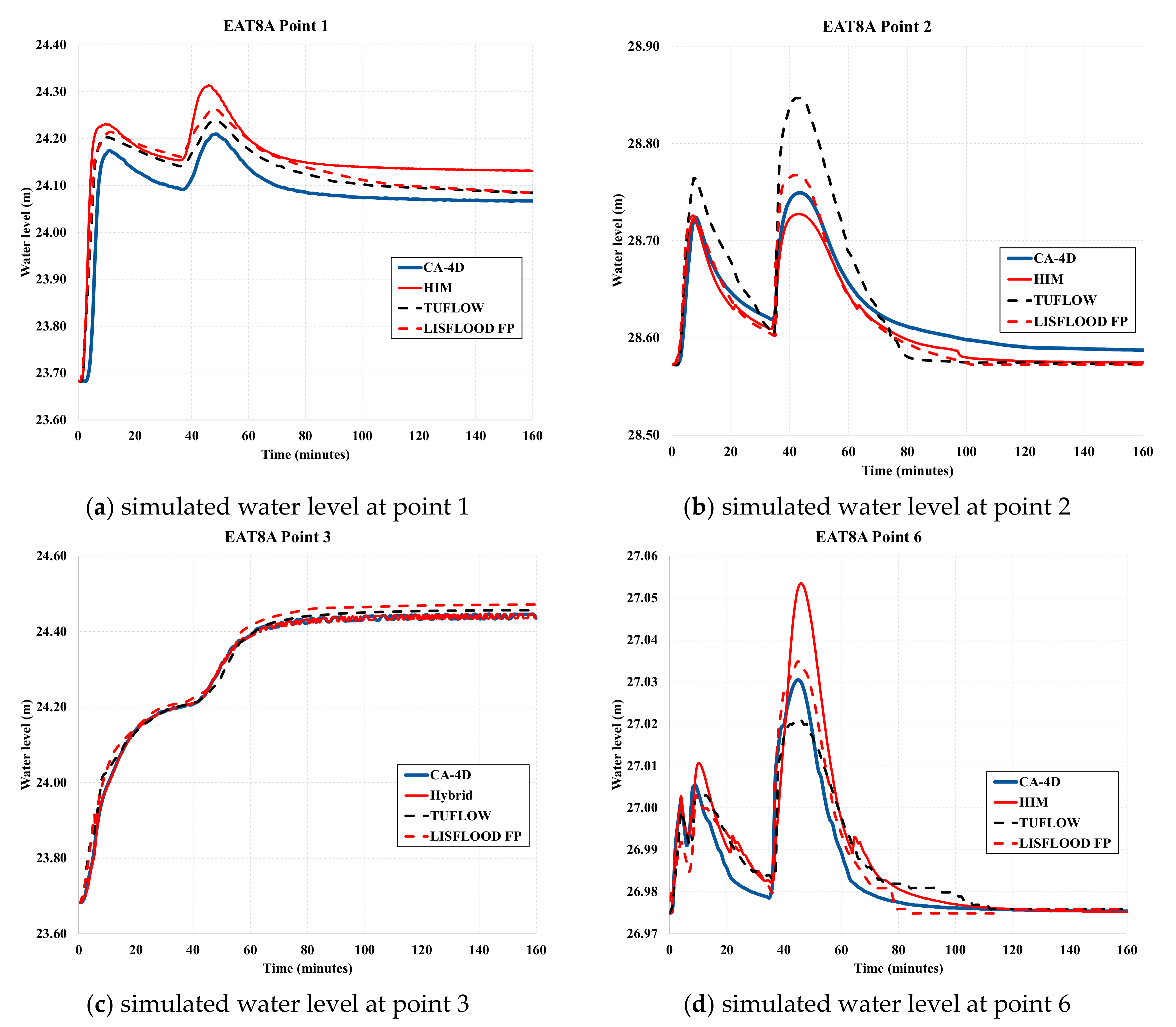
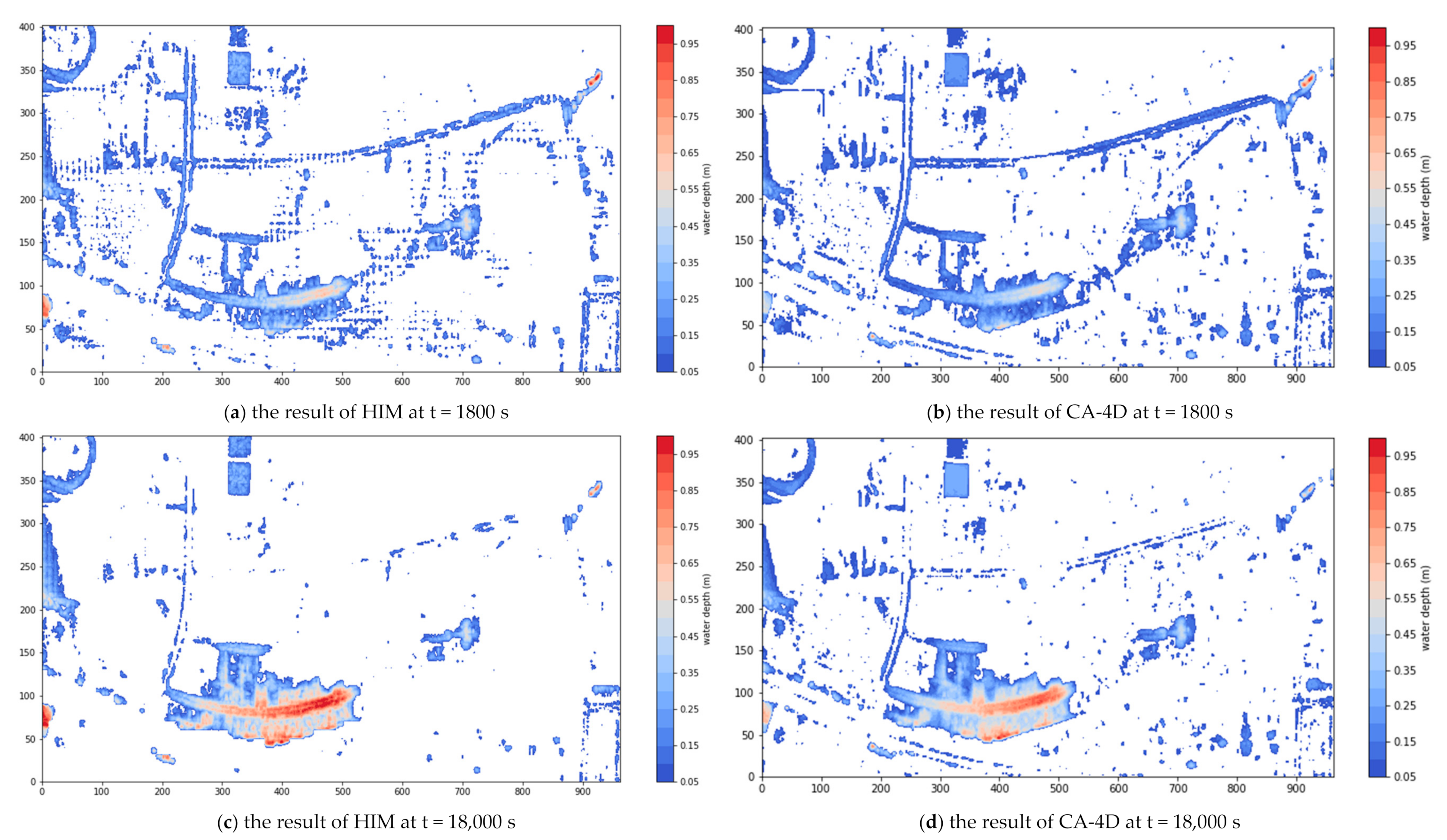
4.1. Three UK EA Benchmark Test Cases
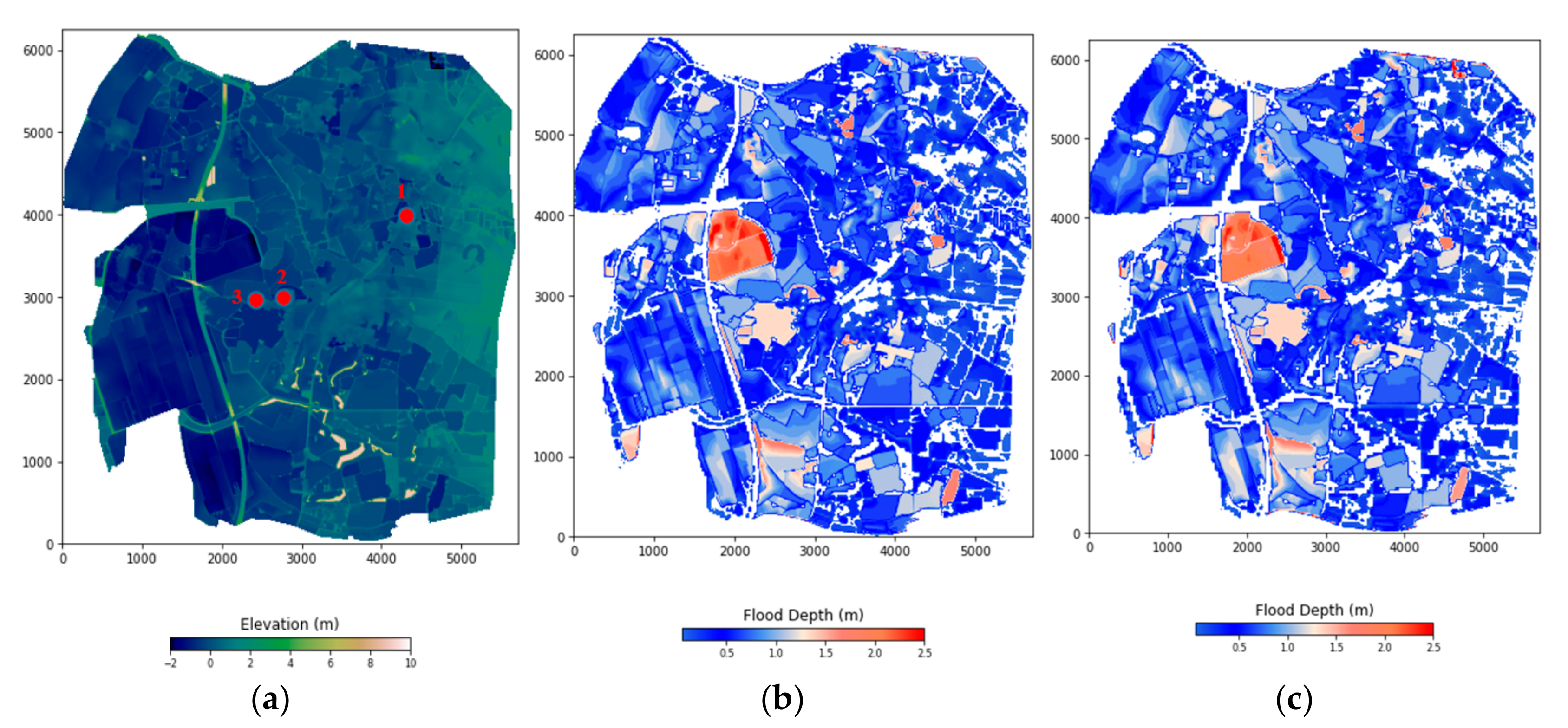
4.2. Coastal Areas of Chiayi County
4.3. Model Efficiency
5. Conclusions
Author Contributions
Funding
Informed Consent Statement
Data Availability Statement
Acknowledgments
Conflicts of Interest
References
- Mizutori, M.; Guha-Sapir, D. Economic Losses, Poverty and Disasters 1998–2017; United Nations Office for Disaster Risk Reduction: Geneva, Switzerland, 2017. [Google Scholar] [CrossRef]
- Luo, T.; Maddocks, A.; Iceland, C.; Ward, P.; Winsemius, H. World’s 15 Countries with the Most People Exposed to River Floods. Available online: http://www.wri.org/blog/2015/03/world%E2%80%99s-15-countries-most-people-exposed-river-floods (accessed on 16 March 2021).
- Albano, R.; Sole, A.; Adamowski, J.; Mancusi, L. A GIS-based model to estimate flood consequences and the degree of accessibility and operability of strategic emergency response structures in urban areas. Nat. Hazards Earth Syst. Sci. 2014, 14, 2847–2865. [Google Scholar] [CrossRef]
- Galland, J.C.; Goutal, N.; Hervouet, J.M. TELEMAC: A new numerical model for solving shallow water equations. Adv. Water Resour. 1991, 14, 138–148. [Google Scholar] [CrossRef]
- Innovyze. InfoWorks ICM Help v3.0. Available online: https://help.innovyze.com/display/infoworksicm/InfoWorks+ICM+Help+Documentation (accessed on 16 March 2021).
- DHI Software. MIKE FLOOD. Available online: https://www.mikepoweredbydhi.com/products/mike-flood (accessed on 7 June 2019).
- Henonin, J.; Russo, B.; Mark, O.; Gourbesville, P. Real-time urban flood forecasting and modelling—A state of the art. J. Hydroinform. 2013, 15, 717–736. [Google Scholar] [CrossRef]
- Lavoie, B.; Mahdi, T.F. Comparison of two-dimensional flood propagation models: SRH-2D and HYDRO_AS-2D. Nat. Hazards 2017, 86, 1207–1222. [Google Scholar] [CrossRef]
- Ginting, B.M.; Mundani, R.P. Parallel flood simulations for wet–dry problems using dynamic load balancing concept. J. Comput. Civ. Eng. 2019, 33, 04019013. [Google Scholar] [CrossRef]
- Huxley, C.; Syme, B. TUFLOW GPU-best practice advice for hydrologic and hydraulic model simulations. In Proceedings of the 37th Hydrology & Water Resources Symposium 2016: Water, Infrastructure and the Environment, Queenstown, New Zealand, 28 November–2 December 2016; Engineers Australia: Queenstown, New Zealand, 2016; p. 195. [Google Scholar]
- Lamb, R.; Crossley, M.; Waller, S. A fast two-dimensional floodplain inundation model. Proc. Inst. Civ. Eng. Water Manag. 2009, 162, 363–370. [Google Scholar] [CrossRef]
- Guidolin, M.; Chen, A.S.; Ghimire, B.; Keedwell, E.C.; Djordjević, S.; Savić, D.A. A weighted cellular automata 2D inundation model for rapid flood analysis. Environ. Model. Softw. 2016, 84, 378–394. [Google Scholar] [CrossRef]
- Bates, P.D.; Horritt, M.S.; Fewtrell, T.J. A simple inertial formulation of the shallow water equations for efficient two-dimensional flood inundation modelling. J. Hydrol. 2010, 387, 33–45. [Google Scholar] [CrossRef]
- Bates, P.D.; De Roo, A.P.J. A simple raster-based model for flood inundation simulation. J. Hydrol. 2000, 236, 54–77. [Google Scholar] [CrossRef]
- Hunter, N.M.; Horritt, M.S.; Bates, P.D.; Wilson, M.D.; Werner, M.G.F. An adaptive time step solution for raster-based storage cell modelling of floodplain inundation. Adv. Water Resour. 2005, 28, 975–991. [Google Scholar] [CrossRef]
- Bradbrook, K.F.; Lane, S.N.; Waller, S.G.; Bates, P.D. Two dimensional diffusion wave modelling of flood inundation using a simplified channel representation. Int. J. River Basin Manag. 2004, 2, 211–223. [Google Scholar] [CrossRef]
- Chen, A.; Djordjević, S.; Leandro, J.; Savic, D. The urban inundation model with bidirectional flow interaction between 2D overland surface and 1D sewer networks. In Proceeding of the 6th NOVATECH International Conference, Lyon, Rhone-Alpes, France, 25–28 June 2007; Workshop I Graie: Lyon, France, 2007; pp. 465–472. [Google Scholar]
- Fewtrell, T.J.; Bates, P.D.; Horritt, M.; Hunter, N.M. Evaluating the effect of scale in flood inundation modelling in urban environments. Hydrol. Process. 2008, 22, 5107–5118. [Google Scholar] [CrossRef]
- Glenis, V.; McGough, A.S.; Kutija, V.; Kilsby, C.; Woodman, S. Flood modelling for cities using cloud computing. J. Cloud Comput. Adv. Syst. Appl. 2013, 2, 7. [Google Scholar] [CrossRef]
- Caviedes-Voullième, D.; Fernández-Pato, J.; Hinz, C. Cellular automata and finite volume solvers converge for 2D shallow flow modelling for hydrological modelling. J. Hydrol. 2018, 563, 411–417. [Google Scholar] [CrossRef]
- Wolfram, S. Cellular automata as models of complexity. Nature 1984, 311, 419–424. [Google Scholar] [CrossRef]
- Blecic, I.; Cecchini, A.; Prastacos, P.; Trunfio, G.; Verigos, E. Modelling urban dynamics with cellular automata: A model of the city of Heraclion. In Proceedings of the 7th AGILE Conference on Geographic Information Science, Heraklion, Greece, 29 April–1 May 2004; University of Crete Press: Heraklion, Greece, 2004. [Google Scholar]
- Pérez-Molina, E.; Sliuzas, R.; Flacke, J.; Jetten, V. Developing a cellular automata model of urban growth to inform spatial policy for flood mitigation: A case study in Kampala, Uganda. Comput. Environ. Urban Syst. 2017, 65, 53–65. [Google Scholar] [CrossRef]
- Freire, J.G.; DaCamara, C.C. Using cellular automata to simulate wildfire propagation and to assist in fire management. Nat. Hazards Earth Syst. Sci. 2018, 19, 169–179. [Google Scholar] [CrossRef]
- D’Ambrosio, D.; Di Gregorio, S.; Iovine, G. Simulating debris flows through a hexagonal cellular automata model: SCIDDICA S3–hex. Nat. Hazards Earth Syst. Sci. 2003, 3, 545–559. [Google Scholar] [CrossRef]
- Iovine, G.; Di Gregorio, S.; Lupiano, V. Debris-flow susceptibility assessment through cellular automata modeling: An example from 15–16 December 1999 disaster at Cervinara and San Martino Valle Caudina (Campania, Southern Italy). Nat. Hazards Earth Syst. Sci. 2003, 3, 457–468. [Google Scholar] [CrossRef]
- Lupiano, V.; Chidichimo, F.; Machado, G.; Catelan, P.; Molina, L.; Calidonna, C.R.; Straface, S.; Crisci, G.M.; Di Gregorio, S. From examination of natural events to a proposal for risk mitigation of lahars by a cellular-automata methodology: A case study for Vascún valley, Ecuador. Nat. Hazards Earth Syst. Sci. 2020, 20, 1–20. [Google Scholar] [CrossRef]
- Aljoufie, M.; Zuidgeest, M.; Brussel, M.; van Vliet, J.; van Maarseveen, M. A cellular automata-based land use and transport interaction model applied to Jeddah, Saudi Arabia. Landsc. Urban Plan. 2013, 112, 89–99. [Google Scholar] [CrossRef]
- Dottori, F.; Todini, E. A 2D flood inundation model based on cellular automata approach. In Proceedings of the XVIII International Conference on Water Resources, Barcelona, Spain, 21–24 June 2010; Carrera, J., Ed.; CMWR: Barcelona, Spain, 2010. [Google Scholar]
- Dottori, F.; Todini, E. Developments of a flood inundation model based on the cellular automata approach: Testing different methods to improve model performance. Phys. Chem. Earth Parts A/B/C 2011, 36, 266–280. [Google Scholar] [CrossRef]
- Ghimire, B.; Chen, A.S.; Guidolin, M.; Keedwell, E.C.; Djordjević, S.; Savić, D.A. Formulation of a fast 2D urban pluvial flood model using a cellular automata approach. J. Hydroinform. 2013, 15, 676–686. [Google Scholar] [CrossRef]
- Liu, L.; Liu, Y.; Wang, X.; Yu, D.; Liu, K.; Huang, H.; Hu, G. Developing an effective 2-D urban flood inundation model for city emergency management based on cellular automata. Nat. Hazards Earth Syst. Sci. 2015, 15, 381–391. [Google Scholar] [CrossRef]
- Wijaya, O.T.; Yang, T.H. Combining two algorithms as a transition rules for CA-based inundation model. In Proceedings of the 22nd IAHR APD, Saporo, Japan, 15–16 September 2020. [Google Scholar]
- Issermann, M.; Chang, F.J.; Jia, H. Efficient urban inundation model for live flood forecasting with cellular automata and motion cost fields. Water 2020, 12, 1997. [Google Scholar] [CrossRef]
- Topa, P.; Młocek, P. GPGPU implementation of cellular automata model of water flow. In Proceedings of the International Conference on Parallel Processing and Applied Mathematics, Torun, Poland, 11–14 September 2011. [Google Scholar]
- Chen, J.; Hill, A.A.; Urbano, L.D. A GIS-based model for urban flood inundation. J. Hydrol. 2009, 373, 184–192. [Google Scholar] [CrossRef]
- CH2M. ISIS FAST. Available online: http://help.floodmodeller.com/isis/ISIS_Fast.htm (accessed on 16 March 2021).
- Yang, T.H.; Chen, Y.C.; Chang, Y.C.; Yang, S.C.; Ho, J.Y. Comparison of different grid cell ordering approaches in a simplified inundation model. Water 2015, 7, 438–454. [Google Scholar] [CrossRef]
- Jamali, B.; Löwe, R.; Bach, P.M.; Urich, C.; Arnbjerg-Nielsen, K.; Deletic, A. A rapid urban flood inundation and damage assessment model. J. Hydrol. 2018, 564, 1085–1098. [Google Scholar] [CrossRef]
- Garcia-Navarro, P. Advances in numerical modelling of hydrodynamics workshop, university of Sheffield, UK, March 24–25, 2015. Appl. Math. Model. 2016, 40, 7423. [Google Scholar] [CrossRef]
- Bates, P.D. Development and testing of a subgrid-scale model for moving boundary hydrodynamic problems in shallow water. Hydrol. Process. 2000, 14, 2073–2088. [Google Scholar] [CrossRef]
- Sanders, B.F.; Schubers, J.E. PRIMo: Parallel raster inundation model. Adv. Water Resour. 2019, 126, 79–95. [Google Scholar] [CrossRef]
- Casulli, V.; Stelling, G.S. Semi-implicit subgrid modelling of three-dimensional free-surface flows. Int. J. Numer. Meth. Fluids. 2010, 67, 441–449. [Google Scholar] [CrossRef]
- Jan, A.; Coon, E.T.; Graham, J.D.; Painter, S.L. A subgrid approach for modelling microtopography effects on overland flow. Water Resour. Res. 2018, 54, 6153–6167. [Google Scholar] [CrossRef]
- Keesstra, S.; Nunes, J.P.; Saco, P.; Parsons, T.; Poeppl, R.; Masselink, R.; Cerdà, A. The way forward: Can connectivity be useful to design better measuring and modelling schemes for water and sediment dynamics? Sci. Total Environ. 2018, 644, 1557–1572. [Google Scholar] [CrossRef]
- Cerdà, A.; Novara, A.; Dlapa, P.; López-Vicente, M.; Úbeda, X.; Popović, Z.; Mekonnen, M.; Terol, E.; Janizadeh, S.; Mbarki, S.; et al. Rainfall and water yield in Macizo del Caroig, Eastern Iberian Peninsula. Event runoff at plot scale during a rare flash flood at the Barranco de Benacancil. Cuad. Investig. Geogr. 2021. [Google Scholar] [CrossRef]
- Néelz, S.; Pender, G. Benchmarking the Latest Generation of 2D Hydraulic Modelling Packages; UK Environment Agency: Rotherham, UK, 2013. [Google Scholar]
- Shen, Y.; Morsy, M.M.; Huxley, C.; Tahvildari, N.; Goodall, J.L. Flood risk assessment and increased resilience for coastal urban watersheds under the combined impact of storm tide and heavy rainfall. J. Hydrol. 2019, 579, 124159. [Google Scholar] [CrossRef]
- Jamali, B.; Bach, P.M.; Cunningham, L.; Deletic, A. A cellular automata fast flood evaluation (CA-ffé) model. Water Resour. Res. 2019, 55, 4936–4953. [Google Scholar] [CrossRef]
- Bennett, N.D.; Croke, B.F.W.; Guariso, G.; Guillaume, J.H.A.; Hamilton, S.H.; Jakeman, A.J.; Marsili-Libelli, S.; Newham, L.T.H.; Norton, J.P.; Perrin, C.; et al. Characterising performance of environmental models. Environ. Model. Softw. 2013, 40, 1–20. [Google Scholar] [CrossRef]
- Hsu, Y.C.; Prinsen, G.; Bouaziz, L.; Lin, Y.J.; Dahm, R. An investigation of DEM resolution influence on flood inundation simulation. Procedia Eng. 2016, 154, 826–834. [Google Scholar] [CrossRef]


| Parameter/Test Case | EAT2 | EAT4 | EAT8A | |||
|---|---|---|---|---|---|---|
| CA-4D | HIM | CA-4D | HIM | CA-4D | HIM | |
| Input Grid Resolution | 20 m | 100 m | 5 m | 20 m | 2 m | 10 m |
| Output Grid Resolution | 20 m | 20 m | 5 m | 5 m | 2 m | 2 m |
| Event Duration | 48 h | 48 h | 5 h | 5 h | 5 h | 5 h |
| Output Frequency | 300 s | 300 s | 20 s | 20 s | 20 s | 20 s |
| α | 0.0125 | 0.5 | 0.02 | 0.2 | 0.0015 | 0.025 |
| ∆tlim | 1 s | 1 s | 1 s | 1 s | 1 s | 1 s |
| Inc_Constant | - | 0.001 m | - | 0.001 m | - | 0.001 m |
| Total Number of Cells | 10,000 | 80,000 | 97,000 | |||
| Observation | C25m | C40m | TUFLOW | |
|---|---|---|---|---|
| Point 1 | 0.775 m | 0.572 m | 0.570 m | 0.513 m |
| Point 2 | 1.100 m | 0.459 m | 0.426 m | 0.506 m |
| Point 3 | 0.000 m | 0.000 m | 0.000 m | 0.030 m |
| RMSE (m) | 0.388 m | 0.407 m | 0.375 m |
| Model | Multiprocessing | Computation Time (min) | ||||
|---|---|---|---|---|---|---|
| UK EA Test Cases | Historical Event | |||||
| EAT2 | EAT4 | EAT8A | C25m | C40m | ||
| CA-4D | No | 136 | 580 | 21,160 | - | - |
| HIM | No | 4.5 | 16.5 | 18.8 | 450 | 71 |
| TUFLOW | Yes -GPU | 0.27 * | 0.42 * | 1.5 * | 480 | |
| LISFLOOD-FP * | Yes | 0.12 * | 0.35 * | 4.5 * | - | |
Publisher’s Note: MDPI stays neutral with regard to jurisdictional claims in published maps and institutional affiliations. |
© 2021 by the authors. Licensee MDPI, Basel, Switzerland. This article is an open access article distributed under the terms and conditions of the Creative Commons Attribution (CC BY) license (https://creativecommons.org/licenses/by/4.0/).
Share and Cite
Wijaya, O.T.; Yang, T.-H. A Novel Hybrid Approach Based on Cellular Automata and a Digital Elevation Model for Rapid Flood Assessment. Water 2021, 13, 1311. https://doi.org/10.3390/w13091311
Wijaya OT, Yang T-H. A Novel Hybrid Approach Based on Cellular Automata and a Digital Elevation Model for Rapid Flood Assessment. Water. 2021; 13(9):1311. https://doi.org/10.3390/w13091311
Chicago/Turabian StyleWijaya, Obaja Triputera, and Tsun-Hua Yang. 2021. "A Novel Hybrid Approach Based on Cellular Automata and a Digital Elevation Model for Rapid Flood Assessment" Water 13, no. 9: 1311. https://doi.org/10.3390/w13091311
APA StyleWijaya, O. T., & Yang, T.-H. (2021). A Novel Hybrid Approach Based on Cellular Automata and a Digital Elevation Model for Rapid Flood Assessment. Water, 13(9), 1311. https://doi.org/10.3390/w13091311